1
Introduction
...
§ 1.1
Motivation
...
China has been undergoing significant social and economic structural changes since launching its policy of economic reform and opening up in 1978. This has involved a transformation from a centrally planned economy, where there is no role for the market, to a market-oriented economy in which market principles play a major role. During the last four decades, great achievements have been made in terms of
economic growth and social well-being. To name a few indicators: the Gross Domestic Product (GDP) of the country increased from USD 189.65 billion in 1980 to USD 10.866 trillion in 2015, positioning China as the second largest economy in the world, with an average annual growth rate over 10%.1Meanwhile, poverty levels have greatly improved. The poverty headcount ratio at USD 1.90 a day (2011 PPP) has decreased dramatically, from 42.15% in 1981 to 10.68% in 2013. The rapid economic growth, combined with the reform of theHukouregistration system, has also accelerated the migration flow from rural areas to urban areas.2The population living in urban China in 2015 reached 763 million, making the urbanisation level of 55.61%, almost three times that in 1980.
With the rapid growth of the urban population, the welfare-based public housing provision system founded in the central planning era could no longer meet the
increasing housing demand of urban residents. Thus, in 1994, comprehensive housing reforms were implemented, aiming to privatize the public housing sector and promote a housing allocation system based on market principles. The milestone of housing reform occurred in 1998, when the government completely suspended the traditional housing allocation system, making the housing market the only way to access housing services (Wang et al. 2012). The emergence of the private urban housing market spurred both housing transactions and prices. In 1998, the housing area traded on the
1 All the data in this paragraph, including GDP, poverty level and urban population, was collected from the World Bank.
2 TheHukou(household registration) system in China was initially designed as a mechanism for monitoring population movements in the early 1950s. Subsequently, it became a strong tool to restrain rural-urban migration and labour mobility between cities.
market was approximately 108 million square metres on an average transaction price of 1854 yuan/m2. These two figures were nearly ten and three times higher in 2014,
soaring to 1.05 billion square metres and 5933 yuan/m2, respectively.3 At the regional level, rapid economic development has been accompanied by increasing inequality. Soon after the launch of the economic reforms, some coastal regions, Guangdong and Zhejiang in Eastern China, for example, grew quickly, due to the influx of foreign direct investment (FDI), advanced technologies and equipment, and favourable policies of the central government. The ‘core’ position of these regions in the national economy was further enhanced through a self-reinforcing process (Anderson 2012, p.127), shaping a core-periphery economic structure in China. In 1980, the regional gross product of Eastern China accounted for 43.69% of total GDP in China, while in 2014 this ratio increased to 51.16%, reflecting the polarization of economic activities .4
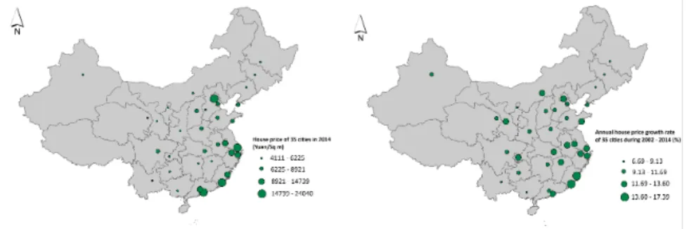
FIGURE 1.1 Spatial distribution of house prices and house price growth rates in 35 cities
Reflecting the distribution of economic activities, the inequality in the cost of housing between regions is also striking. In 2014, the average sale price in 35 main cities in mainland China was approximately 8599 yuan/m2, with the standard error also high,
at 4651 yuan/m2, making the coefficient of variance 0.54, thus indicating a high
degree of heterogeneity across this city-level housing market. The left panel of Figure 1.1 shows the spatial distribution of average house prices. It is apparent that the prices in the coastal cities of Eastern China are generally greater than the prices of inland cities. However, the picture of house price dynamics is a li le different. From 2002 to 2014, the rapid growth in house prices, on average 11.38% per year, seems to be a
3 The housing data used in this section was collected fromChina Statistical Yearbook. Note that the average house prices are calculated without controlling for housing quality.
4 The data for regional economic indicators was collected from the Statistical Yearbook of China and the provinces. Eastern China includes Beijing, Tianjin, Hebei, Shanghai, Jiangsu, Zhejiang, Fujian, Shandong, Guangdong and Hainan.
national phenomenon and there is very li le variance between the annual growth rates in different cities; the coefficient of variance is only 0.18, much lower than that of the house price level. Perhaps the most prominent spatial pa ern of house price growth rate is that the northeastern cities experienced the lowest price appreciation during the period 2002-2014.
This dissertation is fundamentally concerned with the spatial pa erns of house prices and their dynamics across cities in China. Although literature on the Chinese housing market has been emerging in recent years, li le is known about the spatial interaction of regional housing markets. The following four chapters will be dedicated to
responding to questions concerning the emerging market: Why is there a
core-periphery structure in the distribution of interurban house prices? To what extent are the house price developments across cities similar? How do house price dynamics in one city affect the house price changes in other cities?
The investigation of the spatial dimension of the Chinese housing market has been always hampered by the quality of the data, especially when analysing house price dynamics. This situation has inspired the pursuit of research to construct house price indexes that reflect the house price changes as accurately as possible. In line with a key theme of this study, particular a ention has been paid to the influence of the spatial dimension on constructing hedonic imputation house price indexes. Since access to detailed housing transaction records in China is rather restrictive, the analysis in Chapter 6 is based on one housing market in the Netherlands. Using this information, the chapter provides some useful guidance for the construction of house price indexes for Chinese markets.
The remaining sections of this chapter are organised as follows. Section 1.2 provides some background on the formation of the urban private housing market in China, followed by Section 1.3, which briefly reviews the literature on the spatial dimension of house prices. Several questions relating to this research are presented in Section 1.4, while Section 1.5 outlines the structure of the dissertation and briefly introduces the main content of each chapter.
...
§ 1.2
The emergence of an urban private housing market in China
...
After the foundation of the People’s Republic of China in 1949, the country was characterised by a rural-urban dual structure. In urban China, the government gradually established a welfare-oriented housing system through the socialist transformation of private housing and the construction of new public housing. By the late 1970s, the private housing market had almost been eliminated (Huang 2004). In this public rental system, housing was allocated through a work unit-employee linkage.
The rent charged was highly subsidised and the quality of the housing one received relied on a set of non-monetary criteria, such as job rank, job seniority and household size. While this system was beneficial to tenants, it created a huge financial burden and thus restrained housing supply. In 1978, the average housing area consumed per capita in urban China was only 3.6 square metres, which was even below the consumption level in 1949 (Fang et al. 2016).
As China embarked on a transition from a centrally planned economy to a market economy with Chinese characteristics in 1978,5the reform of the housing system was also placed on the agenda, aiming to increase the housing supply. A big step was made in 1988, when land transactions were legally permi ed through a constitutional amendment; however, it should be noted that since land in China belongs to the State, only a land lease right can be transacted on the market.6This reform established the legal basis for private housing construction and the creation of an urban housing market. The housing provision system in urban China subsequently entered a dual structure period, with housing provided either by the public or the private sectors. By 1993, approximately 40% of urban households still resided in state-owned housing (Wang 2011); however, in 1994, the State Council of China introduced a policy to guide work units to sell the public housing to occupying tenants, which significantly
accelerated the public housing privatization process.
The dual structure of housing provision lasted until 1998, when the welfare-oriented housing system was officially discontinued and the market mechanism took control in the allocation of housing. However, government was still involved in two types of housing catering for low-income households. The first was ‘cheap rental housing’ (lianzhu fang), aiming to assist extremely low-income households. The second was ‘affordable housing’ (jingji shiyong fang), which is similar to normal owner-occupied housing except that the construction of affordable housing is subsidised and the price controlled by the government, and with certain restrictions being placed on
transactions. Following these reforms, the rate of home ownership soared to over 80% by 2002 (Wang et al. 2012).
After the establishment of the private urban housing market in the late 1990s, recent years have witnessed the emergence of studies on the operation of this new market. Most of the studies are dedicated to exploring the determinants of house prices and to testing whether there is a house price bubble. The house price fundamentals found in the housing markets of Western countries also play a role in these emerging housing markets. For example, at the national level, monetary policy is thought of as a key
5 The market economy with Chinese characteristics, also known as a socialist market economy, is an economic model which emphasizes the dominance of the state-owned sector but the importance of the market mechanism in the economy.
factor driving national house price changes (Xu and Chen 2012; Zhang et al. 2012). In the cross-city housing market, differences in the population of cities, income levels, the level of air pollution, amenities and supply conditions have been found to be
responsible for the disparities between city house prices (Zheng et al. 2010; Li and Chand 2013; Zheng et al. 2014). Within cities such as Beijing, the monocentric city model can still predict the urban structure to some extent, although a polycentric structure has been emerging in recent years (Zheng and Kahn 2008; Qin and Han 2013). Nevertheless, li le is known about the spatial pa ern of Chinese interurban house prices and their dynamics. The aim of this dissertation is to address this deficit.
...
§ 1.3
The spatial dimension of house prices
...
§ 1.3.1 Spatial distribution of interurban house prices
...
‘Location, location, location’ – the famous mo o of the real estate market – underlines how closely property price is related to property position. Since locations are inherently differentiated in terms of both natural endowments and human activities, it is not a surprise to see certain structures that regulate the distribution of house prices across space. Within an urban area, a common regulatory effect is that, all other things being equal, house price will have a negative relationship with the distance to the central business district (CBD), as depicted by the well-known monocentric city model (Alonso 1964; Mills 1967; Muth 1969). Such a house price gradient has been empirically established in many cities across the world, such as Chicago, Berlin, and Beijing. Of course, a modern city is more than a monocentric city and will be more likely to be characterised by a polycentric structure, in which subcentres and important urban nodes such as hospitals and universities also play a role in shaping the house price pa ern (Heikkila et al. 1989; Waddell et al. 1993). Whether in a monocentric or polycentric city, the house price structure reflects a trade-off between a household’s desire for space and the commuting cost to those urban centres.
Beyond the intra-urban market, how do the house prices differ between urban areas? Note that the focus is on the aggregate house price measured for an entire urban area.7 Before examining the cross-city house price structure, one first needs to determine how the characteristics of a city affect aggregate house prices. In a general spatial equilibrium framework, where the marginal consumer is indifferent across cities, the effect of a city on its house prices should be equivalent to the combined effect that the city has on productivity (wages) and amenity (quality of life) (Roback 1982; Glaeser et
7 For the purpose of house price comparison between cities, an ideal house price measure is the price for an imaginary standard house in a standard location in the city. However, such a measure is rarely available. A commonly used alternative measure is the average price of all houses within the city.
al. 2001). In this regard, the spatial pa ern of cross-city house prices is tied to how the city’s location affects its productivity and amenity.
A framework used to describe the city’s location as well as its effect on productivity and amenity is central place theory, in which cities form an urban hierarchy (Christaller 1933). In the hierarchical system, the higher-tier cities enjoy a productivity and amenity premium not found in the lowest-tier cities. The higher the city is in the hierarchy, the larger the premium. The productivity premium is thought to come from various sources. For example, firms in higher-tier cities are more productive because they can economise on transportation costs in relation to delivering goods and providing services. In addition, the frequent exchange of new ideas in higher-tier cities also benefits productivity. The amenity advantage is mainly due to economies of scale, with some higher-order amenities, such as exotic restaurants, luxury shops and specialised healthcare facilities, only present in higher-tier cities because they need a large market to survive. While the lowest-tier cities do not possess productivity and amenity premiums, they may share in the advantages of these higher-tier cities. The extent to which this can happen depends on their proximity to these higher-tier cities. Therefore, in a hierarchical urban system, house price is expected to decrease with greater distance from higher-tier cities.
In addition, the productivity/amenity advantages/disadvantages of a city might not only depend on its hierarchical position as discussed above, that is, distance to higher-tier cities, but also on its position in the city network, that is, its connection with neighbouring cities generally. The la er view treats the urban system as a network of cities where each interacts with all the others, whether they have a higher-rank, a lower-rank or the same rank (Capello 2000; Boix and Trullén 2007). In the network system, a city’s productivity advantage relates to aggregate and undifferentiated market potential measured by population or income within a broader region, as suggested by New Economic Geography (Fujita et al. 1999; Partridge et al. 2009). In general, greater proximity to larger markets tends to raise factor prices. The amenity advantage of a city in the network relates to the concept of ‘borrowed size’, whereby a city can maintain a higher level of amenities than its own size indicates through borrowing size from the cities within the network; at the same time, the cities which offer the support simultaneously have access to these amenities and thus perform be er than when they are isolated (Meijers and Burger 2015; Meijers et al. 2016). Note that the position in the hierarchy and the position in the city network are not entirely independent, because a higher-tier urban centre always yields larger market potential and higher degree of amenity spillover, but they are complementary to each other in explaining the spatial pa ern of cross-city house prices (Partridge et al. 2009). The house prices of cities are far more complicated than a theoretical model can predict, with elements such as a ‘bubble’ that cannot be explained by fundamentals. The spatial pa ern of bubbles, therefore, partly contributes to the spatial distribution
of house prices. Bubbles are usually not uniformly distributed across space and it is common for bubbles to exist in some cities but not in others. Since housing buyers are not perfectly informed and not rational, they tend to revise their beliefs concerning housing markets through information gained from other agents, a process which can be thought of as ‘social learning’ or ‘social dynamics’(Burnside et al. 2016). In doing so, the optimistic a itudes in bubble markets can easily spread to neighbouring markets and drive up house prices there as well. Such spillovers can result in the spatial clustering of interurban house prices and can be modelled in empirical analysis using spatial econometrics (Fingleton 2008).
§ 1.3.2 Spatial dimension of house price dynamics
...
The house price dynamics of cities are driven by city-specific demand and supply shifters. If the housing supply is elastic and the market is efficient, then, in the long-run, the house price dynamics of a city will only reflect the changes in construction costs (including the cost of land) of that city. However, this is not the whole story in reality, where the housing supply is always constrained by topographical and planning factors and housing markets cannot clear immediately. Thus, it is the interaction of demand and supply shifters that determines the tendency of house prices to change. In addition, common national factors, such as monetary policy and business cycles, are also important determinants of house price dynamics.
Like the house price level, the house price dynamics of cities also have a spatial dimension. In general, cities that have a close geographical proximity tend to be exposed to similar demand and supply shifters, a similar interaction structure and a similar response to common factors, and hence their house price dynamics are closer to each other than to more distant cities. Clustering homogeneous markets can aid in discovering the spatial pa ern of house price dynamics on a larger scale and in identifying sub-national markets. For example, Abraham et al. (1994) revealed three groups of US metropolitan housing markets, namely the West Coast, East Coast and Central US. This clustering logic is also the basis of many regional analyses of house price dynamics. For example, many UK studies have been carried out on the level of Standard Statistical Regions, and their underlying assumption is that the house price dynamics within the region are virtually identical (MacDonald and Taylor 1993; Alexander and Barrow 1994; Holly et al. 2011). However, these regions, designed for administrative purposes, might not completely correspond to the homogeneous market aggregation. At least, for the commercial housing market in the UK, aggregation according to administrative boundaries is not a good solution (Jackson 2002). Thus, in housing analysis, one should be very careful in choosing the appropriate spatial scale.
Another component of the spatial dimension of house price dynamics is the spatial interrelationships between markets. An important hypothesis related to this issue is
that the relationship between markets will be stable in the long-run, although in the short-run, prices might be quite different (Meen 1996). This hypothesis was proposed due to the observation that North/South house price differences in the UK widened in the 1980s and then narrowed in the 1990s (Giussani and Hadjimatheou 1991). The UK housing economists also adopted a related concept of the ripple effect, whereby house prices first rise in the southeast and then spread to the rest of the country. What are the mechanisms or behavioural reasons behind these phenomena? Meen (1999) offered five explanations: migration, equity transfer, spatial pa erns in the
determinants of house prices, spatial arbitrage and coefficient heterogeneity of regional house price models. Of these explanations, the la er two would be the most plausible.
Although the long-run convergence and ripple effect hypotheses originate from empirical observations, the statistical evidence has failed to reach a consensus. While some studies, such as Meen (1996) and Cook (2003), present evidence favouring these hypotheses in the UK, others cast doubt on them (Drake 1995; Abbo and Vita 2013). These hypotheses have also been tested in other markets outside the UK, such as those of Ireland, Sweden, Australia, South Africa and Malaysia, and again the evidence is mixed. The lack of consensus can partly be a ributed to the confusion of long-run convergence and the ripple effect. While some studies consider long-run convergence as a cointegration relationship which states that the house prices of different regions are tied together in the long-run through an equilibrium relationship (e.g.,MacDonald and Taylor 1993), others argue that, to ensure the convergence, certain constraints should be imposed on the long-run equilibrium relationship (Abbo and Vita 2013). In other words, cointegration is necessary for convergence, but not sufficient. Some studies think of the ripple effect as Granger causality, which merely describes a relationship in which house price changes in certain markets lead house price changes in other markets (Stevenson 2004). Others emphasize a transmission pa ern from leading markets to lagged markets, whereby shocks should first spread to nearby areas, with areas further away taking a longer time to respond (Ashworth and Park 1997). Nevertheless, almost all studies agree that, in the short-run, house price changes in one market can spread to other markets, which is generally defined as a diffusion effect (Pollakowski and Ray 1997).
The long-run convergence discussed above does not imply that house prices are equalized across cities. However, there is another stream of studies focusing on the equalization of city-level house prices, which indicate that properties in areas with lower initial house prices will grow faster in price than those in higher initial price areas. The origins of these studies lie in economic growth theory (e.g.,Solow 1956; Swan 1956). Subject to diminishing returns in capital accumulation, growth theory predicts that economies with different initial conditions will ultimately (absolutely) converge to the same steady-state level of income, with poor economies gradually catching up with the leaders. If one applies this theory to the economy of cities, it is natural to conjecture
that per capita income of different cities will ultimately converge, which further leads to the convergence of house prices across cities. However, Kim and Rous (2012) found li le evidence of overall convergence among US state and metropolitan housing markets, instead revealing a few ‘convergence clubs’. Within each club, the house price disparities between the markets diminish over time, while at the same time, the house price difference between the markets of different clubs might increase. In addition to the US market, the phenomenon of club convergence has also been documented in the UK and Spanish housing markets (Montagnoli and Nagayasu 2015; Blanco et al. 2016). Sometimes the house price disparity between markets diminishes over time after controlling for local characteristics, known as conditional convergence. In such a case, house prices of different markets converge towards some permanent disparity relationships that are determined by the heterogeneity in city-specific house price determinants. An example of conditional convergence can be found in a study by Gyourko and Voith (1992), who revealed that higher priced metropolitan areas in the US tend to have lower appreciation rates after controlling for a local fixed effect and a time-varying national effect.
§ 1.3.3 Spatial dimension in house price index construction
...
The quality-adjusted house price indexes that measure pure temporal house price changes are usually constructed by two methods: the repeat sales model and the hedonic price model. The repeat sales model is interested in pricechangesand has been applied to houses sold at least twice during the study period, which omits many single sales and is prone to sample selection bias (Wang and Zorn 1997). While the repeat sales method satisfactorily controls for housing qualities, especially for the location characteristics, if one is interested in thelevelof house prices and the shadow prices of housing characteristics, the repeat sales model does not work. The hedonic price model is a desirable alternative, which assumes that the price of a dwelling can be recovered by a set of housing characteristics. When constructing house price indexes, three methods can be employed: time-dummy methods, imputation methods and characteristics methods (Hill 2013).8
The challenges in applying hedonic price models to the construction of a house price index concern specifying the correct functional form and choosing the appropriate housing characteristics, with the la er being the larger issue. In general, there are two
8 The time-dummy method estimates a pooled hedonic house price model with time dummies for different periods; the time dummies can be directly used to construct the price index. The imputation method estimates a separate hedonic house price model for each of the periods and imputes the prices of dwellings for each period using the estimated shadow prices. Standard price index formulas, such as Laspeyres and Paasche formulas, are then applied to the imputed prices. The characteristics method is very similar to the imputation method. The key difference is that the characteristics method constructs a hypothetical dwelling and the price index is built on the imputed prices of this hypothetical dwelling.
groups of house price characteristics. Firstly, there are the physical characteristics, with the most common variables used in the literature being floor area, land area, age, number of bedrooms and bathrooms, garage, swimming pool, fireplace and air conditioning (Sirmans et al. 2006). Secondly, there are the location-related
characteristics, such as distance to city centre, distance to parks, and the quality of the local school.
Owing to reasons such as data availability, it is impossible to include all the variables that might exert an influence on house prices into the hedonic model. The omission of location variables in particular is likely to cause spatial dependence, the ignorance of which in the hedonic model will yield inconsistent estimates of parameters, which consequently affects the construction of a house price index. To address these
problems, spatial econometric models, such as the spatial autoregressive model (SAR), which incorporates the weighted average house price of neighbouring cities as a predictor, and the spatial error model (SEM), which directly models the spatial correlation structure of error terms, have been introduced to the hedonic house price framework (e.g.,Can 1992; Can and Megbolugbe 1997). The spatial-augmented hedonic model can then be used to improve the calculation of hedonic house price indexes. Some examples can be found in Hill et al. (2009), Dorsey et al. (2010), Pace et al. (1998) and Tu et al. (2004).
It is widely recognized that the value of a dwelling is comprised of two components: the value of the land on which the structure sits and the value of the structure. Some researchers have been interested in separate land price indexes and structure price indexes, because it is very plausible that these two indexes evolve differently over time. However, estimating the land and structure price indexes is not easy for markets where there are no explicit land transactions. Two methods have been proposed to separately estimate land and structure prices from home sales: the residual approach and the hedonic approach. Both of these approaches assume that the house value can be split into a reproducible structure component and an unreproducible land component which capitalizes the value associated with location. The residual approach derives land value from the difference between property value and the replacement cost of the same structures after accounting for depreciation (Davis and Heathcote 2007; Davis and Palumbo 2008). The hedonic approach, in contrast, simultaneously estimates the value of the structure and the land in a hedonic framework, where the land price refers to the marginal implicit price per unit of land plot (Kuminoff and Pope 2013; de Groot et al. 2015).
However, in practice, the residual approach is more commonly used because the hedonic approach suffers from omi ed variable bias. The houses located in a be er neighbourhood with higher land values tend to have nicer physical structural
characteristics that cannot be readily observed, and therefore the estimated land value will be confounded with the value of unobservable physical characteristics.
Nevertheless, the hedonic approach has one virtue: if estimated correctly, the hedonic principle of value seems more consistent with the notion of market value (Kuminoff and Pope 2013). Therefore, if one wants to take advantage of the hedonic approach, it is necessary to seek a solution to the omi ed variable bias. In particular, the spatial dimension of land values requires be er treatment. A common treatment assumes land prices to be constant within the neighbourhood, recognizing the fact that houses within the neighbourhood are exposed to the same local public goods and amenities. However, it can be argued that this treatment might be too crude and that the price of land plots might vary significantly even within one neighbourhood. Imagining a neighbourhood alongside a lake, it is very likely that the land plots near the lake have higher prices than the land plots further away. Therefore, the spatial dimension of land prices associated with location should be treated more concisely when constructing the price index of land, structure and houses.
...
§ 1.4
Research questions
...
The objective of this dissertation is to draw a comprehensive picture of house price behaviour in the spatial dimension. It is mainly concerned with three aspects involving two spatial scales. On the interurban scale, the spatial distribution of interurban house prices and the spatial relationships of interurban house price dynamics are the main topics. On the intra-urban scale, the focus is on the spatial correlation and
heterogeneity of property prices. In Chapters 2 to 5, a great deal of a ention is paid to interurban housing markets in China. In Chapter 6, the focus is on the intra-city housing market in the Netherlands.
The spatial distribution of interurban house prices is intensively dealt with in Chapters 2 and 3. The key questions that need to be answered are:
What is the spatial distribution of house prices across cities? How can that pa ern be explained? What role does location play in shaping the interurban house price pa ern?
(Chapters 2 and 3)
Chapter 2 a empts to answer these questions from the point of view of the hierarchical urban system, where the top-tier cities provide the entire range of urban products and the lower-tier cities only offer a few. The specific questions relating to this chapter are:
Can an interurban house price gradient, whereby house prices decrease when moving away from the core cities to periphery cities, be observed in the urban hierarchical system? If yes, how can we explain this pa ern? Which factors can it be a ributed to?
(Chapter 2)
paradigm, which nests the possibilities of both hierarchical and non-hierarchical structures (Capello 2000). Therefore, this chapter looks into the spatial distribution of house prices from the perspective of city network externalities. The related questions are:
Do cross-city spillovers, which mean that the house price of one market depends on the market conditions of neighbouring markets, contribute to explaining the spatial clustering pa ern of interurban house prices? If so, is city network externality one of the channels that generate such spillovers?(Chapter 3)
Chapters 4 and 5 are concerned with the spatial dimension of interurban house price dynamics. The general questions related to this are:
Are house price dynamics across cities different from each other or are they homogeneous? What are the long-run and short-run relationships between them?
(Chapter 4 and 5)
Chapter 4 investigates the national interurban housing market and focuses on the overall heterogeneous (or homogeneous) house price dynamics across cities and structural changes across different sub-periods. The main sub-questions in this chapter are:
Can city house price dynamics be divided into a few homogeneous clusters within which the cities have similar house price growth trajectories? Are there structural changes such that the cluster memberships are not consistent across different periods? Can
geography play a role in explaining the cluster structure?(Chapter 4)
Chapter 5 pays more a ention to the relative relationships between housing market dynamics, such as the leading-lag relationships, and, long-run and short-run relationships. These aspects are reflected in the questions:
Is there any leading-lag relationship across the city housing markets such that the historical house price information in one market can be used to predict the current house prices in other markets? Has a long-run equilibrium relationship been
maintained such that the markets will not deviate from each other? Is there a distinct house price diffusion pa ern in the short-run such that shocks to one particular market gradually propagate to other markets?(Chapter 5)
Chapter 6 deals with the construction of a house price index, which measures the house price development of a city. Particular a ention is paid to the impact of spatial characteristics on the house price index. The questions related to this chapter are:
How can the house price index be decomposed into a land price index and a structure price index? Does be er treatment of location benefit the construction of a house price
index?(Chapter 6)
...
§ 1.5
Introduction to chapters
...
Each of the chapters following this introduction responds to the corresponding questions raised in Section 1.4 above. Figure 1.2 below outlines the structure of the dissertation and the theories and/or methodologies used in each chapter. A detailed introduction to each chapter can also be found below.
FIGURE 1.2 Outline of the chapters
Chapters 2 and 3 are mainly concerned with the spatial distribution of interurban house prices within the urban system of the Pan-Yangtze River Delta (PYRD) in Eastern China, which includes 42 cities. A panel data set was compiled from various sources for these two chapters. Chapter 2 treats this urban system as a hierarchical urban system, in which one city is deemed to be the top-tier city, three cities to be second-tier cities and all the other cities to be third-tier (lowest-tier) cities. Based on Central Place Theory, which asserts that higher-tier cities will be more productive and produce more urban functions than lower-tier cities (Partridge et al. 2009), the general spatial equilibrium model of Rosen-Roback (Rosen 1979; Roback 1982) demonstrates that the further a city is from the higher-tier cities, the lower the house prices in that city. This negative interurban house price gradient is shaped by two channels: a ‘productive component’, whereby the more distant cities receive less agglomeration spillovers from higher-tier cities, and an ‘amenity component’, whereby it is more costly for the more peripheral cities to gain access to higher-order amenities. The interurban house price gradients in relation to higher-tier cities are then empirically estimated in terms of the urban system of PYRD, and they are further decomposed into the productivity
component and amenity component so that the relative contribution of these two components can be assessed.
Chapter 3 understands the urban system through the paradigm of a city network system, within which a city can ‘borrow size’ from neighbouring cities, allowing that city to achieve be er performance in terms of productivity and amenity than is indicated by its size (Alonso 1973; Meijers and Burger 2015). Such city network externalities will generate some cross-city spillovers, such that having good access to larger neighbouring markets tends to increase house prices. Based on the urban system of PYRD, the city network externalities in the housing market are empirically modelled using the methods of spatial econometrics, in which the spatial interaction structure is captured by a spatial weight matrix. Specifically, the spatial lag of X model (SLX), which includes the spatial lags of independent variables, and the spatial Durbin error model (SDEM), which captures the spatial lag information of both independent variables and error terms, are employed. These two models can reveal the relationship between one city’s house price and the urban size of neighbouring cities, which carries information about city network spillovers. In general, the cross-city spillovers of housing markets – that is, the house price of a city being dependent on the housing market conditions of neighbouring cities – may be raised not only by city network externality, but also by other channels, such as yardstick competitions (Brady 2014).9 In this sense, another two common approaches, the spatial autoregressive model (SAR), which incorporates the spatial lag of dependent variable, and the spatial Durbin model (SDM), which includes the spatial lags of both dependent and independent variables, are also estimated. However, these two methods are hard to be theoretically justified, and thus suffer from the identification problem (Gibbons and Overman 2012).
Chapters 4 and 5 both deal with the spatial dimension of house price dynamics but with different focuses. Chapter 4 is dedicated to the overall clustering pa erns of house price dynamics across the whole country based on some similarity measures.
Specifically, it a empts to group the housing markets of 34 major Chinese cities –which are either municipalities directly controlled by the central government, capitals of provinces or vital economic centres –into a few clusters according to the house price appreciation trajectories from 2005 July to 2016 June. The data are extracted from the ‘Price Indices of Newly Constructed Residential Buildings in 35/70 Large- and Medium-sized Cities’, in which the quality changes have been controlled for to some extent, published monthly by the National Bureau of Statistics of China (NBSC). Before performing the cluster analysis, a measure that reflects the degree of similarity between housing markets must be defined, such as the Euclidean distance. This chapter, being different from the literature, adopts a distribution-based dissimilarity measure – Kullback-Leibler (KL) divergence (Kullback 1968), which has been applied in
9 Yardstick competition in housing markets simply means that market participants in one market compete with participants in the neighbouring markets such that the house price formation processes in these markets are correlated with each other.
machine learning and environmental studies but not in housing analysis. TheKL
divergence has a probability meaning and thus can allow one to make inferences, while Euclidean distance does not. The homogeneous clusters are then obtained using the hierarchical agglomerative clustering method, which has been extensively used in the literature on the homogeneous grouping of commercial markets. Considering the changing conditions of Chinese housing markets, structural changes are also tested to see whether or not the cluster membership is consistent throughout the period. To do so, the sample period is split into three sub-periods and the cluster analysis is performed on each sub-sample. Furthermore, this chapter closely examines the effectiveness of two commonly used classification schemes in describing the
interurban housing market structure in China – the geographical demarcation system defined by NBSC and the city-tier system published by various institutes.
In order to carefully examine the relative relationships between housing markets, Chapter 5 concentrates on the housing markets of ten vital cities in a common economic area in South China – the Pan-Pearl River Delta (Pan-PRD), which includes cities from developed Eastern China and less developed Central and Western China. The NBSC monthly price indexes are also used, covering the period from June 2005 to May 2015. The first question regarding the relative relationship between housing markets concerns whether the house price change information in some markets leads the house prices changes in other markets. The leading-lag relationships of housing markets are examined using the Toda-Yamamoto Granger causality test (Toda and Yamamoto 1995). Compared to the standard Granger causality procedure, the Toda-Yamamoto procedure is more flexible and powerful. Subsequently, the long-run equilibrium relationship between housing markets is investigated. If the house price ratio between two markets moves around a constant level in the long-run, the two housing markets are then considered to be convergent. The long-run convergence properties between pairwise housing markets are investigated using the Engle-Granger cointegration test, with certain restrictions imposed on the cointegration space. Finally, a house price diffusion model that considers both the long-run and short-run spatial relationships is built. In this diffusion model, the house price growth of a city at time depends not only on its own lagged price changes, but also on the lagged price changes of its neighbours and on the long-run equilibrium relationship with neighbours. In particular, the house price information of neighbours is synthesized using a spatial weight matrix. This model is a variant of that of Holly et al (2011), and, combined with the General Impulse Response Function (GIRF), presents a full picture of the house price behaviour between markets.
Chapter 6 switches the focus from the interurban housing market to an intra-urban housing market, and is concerned with the construction of a house price index, which is the input for the analysis of interurban house price dynamics. Since access to housing transactions in the Chinese market is not available, this chapter is based on a small city in the Netherlands. The chapter starts with a ‘builder’s model’, which decomposes the
value of a dwelling into the value of the structure and the value of the land. The land component is of particular interest because location characteristics are mainly capitalized intoland values. As such, land prices are expected to vary significantly within the whole market, even within the neighbourhood, whereas the implicit price of structural characteristics will be the same across space. To capture these features, this chapter applies a mixed geographically weighted regression (MGWR) model, which models the land prices in a nonparametric fashion and the structural prices in a parametric fashion. Specifically, the nonparametric part of the MGWR model assumes that the land price of a location depends on neighbouring land prices, whereby both the spatial dependence and spatial heterogeneity of land prices can be properly dealt with. Another two restrictive models are also estimated, with one assuming that land prices are fixed across the city-wide markets and the other assuming that land prices vary across neighbourhoods. The performance of these three models is then
comprehensively assessed. Most importantly, various hedonic imputation house price indexes, land price indexes and structural price indexes are compiled based on the estimates of these three models and the differences between indexes generated by different models are investigated. To simplify the treatment of land component, this analysis mainly uses the sales of single-family dwellings. For the apartments, some special treatment is needed to extract the land component. However, the essence of the model is indifferent to the dwelling types. In this regard, the model presented in this chapter is still enlightening about the construction of separate price indexes for Chinese markets.
...
References
...
Abbo , A., & Vita, G. D. (2013). Testing for long-run convergence across regional house prices in the UK: A pairwise approach. Applied Economics, 45(10), 1227-1238.
Abraham, J. M., Goetzmann, W. N., & Wachter, S. M. (1994). Homogeneous groupings of metropolitan housing markets. Journal of Housing Economics, 3(3),
186-206.
Alexander, C., & Barrow, M. (1994). Seasonality and cointegration of regional house prices in the UK. Urban Studies, 31(10), 1667-1689.
Alonso, W. (1964). Location and land use: toward a general theory of land rent. Cambridge MA: Harvard University Press.
Alonso, W. (1973). Urban zero population growth. Daedalus, 102(4), 191-206. Anderson, W. P. (2012). Economic Geography. Abingdon,Oxfordshire: Routledge. Ashworth, J., & Park, S. C. (1997). Modeling regional house prices in the UK. Sco ish
Journal of Political Economy, 44(3), 225-246.
Spanish during the housing boom. Urban Studies, 53(4), 775-798. Boix, R., & Trullén, J. (2007). Knowledge, networks of cities and growth in regional
urban systems. Papers in Regional Science, 86(4), 551-574.
Brady, R. R. (2014). The spatial diffusion of regional housing prices across U.S. states. Regional Science and Urban Economics, 46, 150-166.
Burnside, C., Eichenbaum, M., & Rebelo, S. (2016). Understanding booms and busts in housing markets. Journal of Political Economy, forthcoming.
Can, A. (1992). Specification and estimation of hedonic housing price mdoels. Regional Science and Urban Economics, 22(3), 453-474.
Can, A., & Megbolugbe, I. (1997). Spatial dependence and house price index
construction. Journal of Real Estate Finance and Economics, 14(1-2), 203-222. Capello, R. (2000). The city network paradigm: Measuring urban network externalities.
Urban Studies, 37(11), 1925-1945.
Christaller, W. (1933). Central places in Southern Germany. (translated by C.W.Baskin,1966). London: Prentice Hall.
Cook, S. (2003). The convergence of regional house prices in the UK. Urban Studies, 40(11), 2285-2294.
Davis, M. A., & Heathcote, J. (2007). The price and quantity of residential land in the United States. Journal of Monetary Economics, 54(8), 2595-2620.
Davis, M. A., & Palumbo, M. G. (2008). The price of residential land in large US cities. Journal of Urban Economics, 63(1), 352-384.
de Groot, H. L. F., Marlet, G., Teulings, C., & Vermeulen, W. (2015). Cities and the Urban Land Premium. Cheltenham: Eaward Elgar.
Dorsey, R. E., Hu, H., Mayer, W. J., & Wang, H. (2010). Hedonic versus repeat-sales housing price indexes for measuring the recent boom-bust cycle. Journal of Housing Economics, 19(2), 75-93.
Drake, L. (1995). Testing for convergence between UK regional house prices. Regional Studies, 29(4), 357-366.
Fang, H., Gu, Q., Xiong, W., & Zhou, L. (2016). Demystifying the Chinese housing boom. In M. Eichenbaum, & J. Parker (Eds.), NBER Macroeconomics Annual 2015 (Vol. 30, pp. 105-166). Chicago: University of Chicago Press. Fingleton, B. (2008). Housing supply, housing demand, and affordability. Urban
Studies, 45(8), 1545-1563.
Fujita, M., Krugman, P., & Mori, T. (1999). On the evolution of hierarchical urban systems. European Economic Review, 43(2), 209-251.
Gibbons, S., & Overman, H. G. (2012). Mostly pointless spatial econometrics? Journal of Regional Science, 52(2), 172-191.
Giussani, B., & Hadjimatheou, G. (1991). Modeling regional house prices in the United Kingdom. Papers in Regional Science, 70(2), 201-219.
Glaeser, E. L., Kolko, J., & Saiz, A. (2001). Consumer city. Journal of Economic Geography, 1(1), 27-50.
appreciation. Journal of Urban Economics, 32(1), 52-69.
Heikkila, E., Gordon, P., Kim, J. I., Peiser, R. B., Richardson, H. W., & Dale-Johnson, D. (1989). What happened to the CBD-distance gradient? Land values in a policentric city. Environment and Planning A, 21(2), 221-232.
Hill, R. J. (2013). Hedonic Price Indexes for Residential Housing: A Survey, Evaluation and Taxonomy. Journal of Economic surveys, 27(5), 879-914.
Hill, R. J., Melser, D., & Syed, I. (2009). Measuring a boom and bust: The Sydney housing market 2001 - 2006. Journal of Housing Economics, 18(3), 193-205. Holly, S., Pesaran, M. H., & Yamagata, T. (2011). The spatial and temporal diffusion of
house prices in the UK. Journal of Urban Economics, 69(1), 2-23. Huang, Y. (2004). The road to homeownership: a longitudinal analysis of tenure
transition in urban China (1949-94). International Journal of Urban and Regional Research, 28(4), 774-795.
Jackson, C. (2002). Classifying local retail property markets on the basis of rental growth rates. Urban Studies, 39(8), 1417-1438.
Kim, Y. S., & Rous, J. J. (2012). House price convergence: Evidence from US state and metropolitan area panels. Journal of Housing Economics, 21(2), 169-186. Kullback, S. (1968). Information theory and statistics. New York: Dover Publications. Kuminoff, N. V., & Pope, J. C. (2013). The value of residential land and structures
during the great housig boom and bust. Land Economics, 89(1), 1-29. Li, Q., & Chand, S. (2013). House prices and market fundamentals in urban China.
Habitat International, 40, 148-153.
MacDonald, R., & Taylor, M. P. (1993). Regional house prices in Britain: long-run relationships and short-run dynamics. Sco ish Journal of Political Economy, 40(1), 43-55.
Meen, G. (1996). Spatial aggregation, spatial dependence and predictability in the UK housing market. Housing Studies, 11(3), 345-372.
Meen, G. (1999). Regional house prices and the ripple effect: A new interpretation. Housing Studies, 14(6), 733-753.
Meijers, E. J., & Burger, M. J. (2015). Stretching the concept of ’borrowed size’. Urban Studies, Forthcoming.
Meijers, E. J., Burger, M. J., & Hoogerbrugge, M. M. (2016). Borrowing size in networks of cities: City size, network connectivity and metropolitan functions in Europe. Papers in Regional Science, 95(1), 181-199.
Mills, E. S. (1967). An aggregation model of resource allocation in a metropolitan area. American Economic Review, 57(2), 197-210.
Montagnoli, A., & Nagayasu, J. (2015). UK house price convergence clubs and spillovers. Journal of Housing Economics, 30, 50-58.
Muth, R. F. (1969). Cities and housing: the spatial pa ern of urban residential land use. Chicago: University of Chicago Press.
Pace, R. K., Barry, R., Clapp, J. M., & Rodriquez, M. (1998). Spatiotemporal
and Economics, 17(1), 15-33.
Partridge, M. D., Rickman, D. S., Ali, K., & Olfert, M. R. (2009). Agglomeration spillovers and wage and housing cost gradients across the urban hierarchy. Journal of International Economics, 78(1), 126-140.
Pollakowski, H. O., & Ray, T. S. (1997). Housing price diffusion pa erns at different aggregation levels: An examination of housing market efficiency. Journal of Housing Research, 8(1), 107-124.
Qin, B., & Han, S. S. (2013). Emerging polycentricity in Beijing: Evidence from housing price variations,2001-05. Urban Studies, 50(15), 2006-2023.
Roback, J. (1982). Wages, rents, and the quality of life. Journal of Political Economy, 90(6), 1257-1278.
Rosen, S. (1979). Wage-based indexes of urban quality of life. In P. Mieszkowski, & M. Straszheim (Eds.), Current Issues in Urban Economics. Baltimore: The Johns Hopkins University Press.
Sirmans, G. S., MacDonald, L., Macpherson, D. A., & Zietz, E. N. (2006). The value of housing characteristics: A meta analysis. The Journal of Real Estate Finance and Economics, 33(3), 215-240.
Solow, R. M. (1956). A contribution to the theory of economic growth. Quarterly Journal of Economics, 70(1), 65-94.
Stevenson, S. (2004). House price diffusion and inter-regional and cross-border house price dynamics. Journal of Property Research, 21(4), 301-320.
Swan, T. W. (1956). Economic growth and capital accumulation. Economic Record, 32(2), 334 - 361.
Toda, H. Y., & Yamamoto, T. (1995). Statistical inference in vector autoregressions with possibly integrated processes. Journal of Econometrics, 66, 225-250.
Tu, Y., Yu, S.-M., & Sun, H. (2004). Transaction-Based Office Price Indexes: A Spatiotemporal Modeling Approach. Real Estate Economics, 32(2), 297-328. Waddell, P., Berry, B. J. L., & Hoch, I. (1993). Residential property values in a
multinodal urban area: New evidence on the implicit price of location. Journal of Real Estate Finance and Economics, 7(2), 117-141.
Wang, F. T., & Zorn, P. M. (1997). Estimating house price growth with repeat sales data: What’s the aim of the game? Journal of Housing Economics, 6(2), 93-118. Wang, S.-Y. (2011). State misallocation and housing prices: Theory and evidence from
China. American Economic Review, 101(5), 2081-2107.
Wang, Y., Shao, L., Murie, A., & Cheng, J. (2012). The maturation of the neo-liberal housing market in urban China. Housing Studies, 27(3), 343-359.
Xu, X. E., & Chen, T. (2012). The effect of monetary policy on real estate price growth in China. Pacific-Basin Finance Journal, 20(1), 62-77.
Zhang, Y., Hua, X., & Zhao, L. (2012). Exploring determinants of housing prices: A case study of Chinese experience in 1999 - 2010. Economic Modelling, 29(6), 2349-2361.
cross-boundary air pollution externalities: Evidence from Chinese cities. Journal of Real Estate Finance and Economics, 48(3), 398-414.
Zheng, S., & Kahn, M. E. (2008). Land and residential property markets in a booming economy: New evidence from Beijing. Journal of Urban Economics, 63(2), 743-757.
Zheng, S., Kahn, M. E., & Liu, H. (2010). Towards a system of open cities in China: Home prices, FDI flows and air quality in 35 major cities. Regional Science and Urban Economics, 40(1), 1-10.