CPz : classification-aided photometric-redshift estimation.

Deposited in DRO:

Version of attached le:

Peer-review status of attached le:

Citation for published item:

Fotopoulou, S. and Paltani, S. (2018) 'CPz : classication-aided photometric-redshift estimation.', Astronomy astrophysics., 619 . A14.

Further information on publisher's website:

Publisher's copyright statement:

Reproduced with permission from Astronomy Astrophysics, cESO. Additional information:

Use policy

The full-text may be used and/or reproduced, and given to third parties in any format or medium, without prior permission or charge, for personal research or study, educational, or not-for-prot purposes provided that:

• a full bibliographic reference is made to the original source

• alinkis made to the metadata record in DRO

• the full-text is not changed in any way

The full-text must not be sold in any format or medium without the formal permission of the copyright holders. Please consult thefull DRO policyfor further details.

Durham University Library, Stockton Road, Durham DH1 3LY, United Kingdom Tel : +44 (0)191 334 3042 | Fax : +44 (0)191 334 2971

A&A 619, A14 (2018) https://doi.org/10.1051/0004-6361/201730763 c ESO 2018

Astronomy

&

Astrophysics

CPz: Classification-aided photometric-redshift estimation

?

S. Fotopoulou

and S. Paltani

1 _{Department of Astronomy, University of Geneva, ch. d’Ecogia 16, 1290 Versoix, Switzerland}

e-mail:[email protected]; [email protected]

2 _{Center for Extragalactic Astronomy, Department of Physics, Durham University, South Road, Durham DH1 3LE, UK}

Received 10 March 2017/Accepted 10 July 2018

ABSTRACT

Broadband photometry offers a time and cost effective method to reconstruct the continuum emission of celestial objects. Thus, photometric redshift estimation has supported the scientific exploitation of extragalactic multiwavelength surveys for more than twenty years. Deep fields have been the backbone of galaxy evolution studies and have brought forward a collection of various approaches in determining photometric redshifts. In the era of precision cosmology, with the upcoming Euclidand LSST surveys, very tight constraints are put on the expected performance of photometric redshift estimation using broadband photometry, thus new methods have to be developed in order to reach the required performance. We present a novel automatic method of optimizing photometric redshift performance, the classification-aided photometric redshift estimation (CPz). The main feature of CPz is the unified treatment of all classes of objects detected in extragalactic surveys: galaxies of any type (passive, starforming and starbursts), active galactic nuclei (AGN), quasi-stellar objects (QSO), stars and also includes the identification of potential photometric redshift catastrophic outliers. The method operates in three stages. First, the photometric catalog is confronted with star, galaxy and QSO model templates by means of spectral energy distribution fitting. Second, three machine-learning classifiers are used to identify 1) the probability of each source to be a star, 2) the optimal photometric redshift model library set-up for each source and 3) the probability to be a photometric redshift catastrophic outlier. Lastly, the final sample is assembled by identifying the probability thresholds to be applied on the outcome of each of the three classifiers. Hence, with the final stage we can create a sample appropriate for a given science case, for example favoring purity over completeness. We apply our method to the near-infrared VISTA public surveys, matched with optical photometry from CFHTLS, KIDS and SDSS, mid-infrared WISE photometry and ultra-violet photometry from the Galaxy Evolution Explorer (GALEX). We show that CPz offers improved photometric redshift performance for both normal galaxies and AGN without the need for extra X-ray information.

Key words. methods: data analysis – stars: general – galaxies: general – galaxies: active – surveys

1. Introduction

Looking at a single broadband image, obtained for example in therband (6000 Å), we are able to distinguish distinct sources

and classify them according to their morphologies, ranging from round and smooth elliptical galaxies to the impressive grand design spiral galaxies (Hubble 1926). We now know that the morphologies are linked to the type of stellar populations and the gas and dust content of the galaxy. For example, passive galaxies are known to consist of mainly old star populations, while star-forming galaxies consist of younger, bluer stars pop-ulating the galaxy’s spiral arms. However, from a single image we can not say with certainty for example if a point-like source is really a star or a quasi-stellar object (QSO), or what is the cosmological distance of the source. Source classification has been subsequently enhanced by attributes both from photometric (e.g., colors) and spectroscopic (e.g., line widths) measurements. Plotting pairs of attributes has proven to be a powerful tool in identifying the parameter space occupied by each galaxy class for example separating between starforming and passive galax-ies using the bimodality cloud (Bell et al. 2004), or separating between starforming galaxies and active galactic nuclei (AGN) through the BPT diagram (Baldwin et al. 1981). The main lim-? _{The catalog is only available at the CDS via anonymous ftp to} cdsarc.u-strasbg.fr (130.79.128.5) or via http://cdsarc. u-strasbg.fr/viz-bin/qcat?J/A+A/619/A14

itation of this approach is the dimensionality reduction of a wealthy parameter space to usually only two to four attributes and the introduction of hard limits to separate between the classes.

Another approach in identifying the nature of astronomical sources is the comparison of stellar population synthesis models (SSP) to observations through spectral energy distribution (SED) fitting. SSPs demonstrate that the age and metallicity of the star population will create a distinct galaxy continuum emission which can be probed with broadband photometry which however suffers from degeneracies in color space (e.g.,Bruzual & Charlot 2003;Maraston 2005). A selection of models deemed represen-tative of the sample at hand can be used to identify stars vs galaxies and to estimate physical properties such as the stellar mass, star-formation rate, amongst others, judged by least χ2 (e.g.,Bolzonella et al. 2000;Robin et al. 2007;Ilbert et al. 2009; Fotopoulou et al. 2012; Dahlen et al. 2013). Lastly, machine-learning algorithms are very well applicable to an astronomi-cal context and they have been embraced since the early 90’s. supervised and unsupervised methods are able to identify corre-lations, groupings and even outliers in vast datasets that would otherwise be impossible to visualize by a human eye. Many works have explored classification in astronomy using machine-learning techniques aiming towards separating stars from galax-ies (Odewahn et al. 1993; Soumagnac et al. 2015), QSO iden-tification (Brescia et al. 2015), estimating physical parameters

(Ucci et al. 2017), finding peculiar objects (Meusinger et al. 2012), etc.

In addition to the class of the object, multiwavelength infor-mation are useful in providing an estimate of the redshift as proposed by Baum (1962). All modern extragalactic surveys make extensive use of photometric redshift estimation as it is a cost-efficient method to determine distances of galaxies (COMBO-17, CFHTLS, CDFS and ECDFS, Lockman Hole, AEGIS, COSMOS, XXL, to name a few). However, most sur-veys are mainly focused on the normal galaxy population. In the presence of deep X-ray flux measurements, variability and mor-phology information,Salvato et al.(2009,2011) showed that the optimal photometric redshift solution can be achieved by dis-secting the galaxy population in three categories containing 1) normal galaxies, 2) normal galaxy and AGN emission, 3) AGN dominated emission, which we refer to as QSO. This method has been successfully applied to other extragalactic fields such as the Lockman Hole (Fotopoulou et al. 2012), theChandraDeep

Field South (Hsu et al. 2014) and AEGIS-X (Nandra et al. 2015) and it is the current state of the art, used when X-ray data are available for the whole field in consideration. The core of the method is the use of independent information such as X-ray flux, morphology and variability to pin-point the SED mod-els that will give the optimal photometric redshift solution for each population. By doing so, the degeneracies between mod-els are reduced, thus achieving higher photometric redshift per-formance. However, the correct implementation of the method requires splitting the sample into point-like and varying sources and also having an estimate of X-ray flux. This information will not be available to the desired sensitivity for the majority of the source population detected byEuclidand LSST.

In this paper, we generalize the idea of population-specific libraries designed for application on surveys for which X-ray fluxes and variability information is not available and the mor-phology is estimated by the half light radius. The classification-aided photometric-redshift estimation (CPz) utilizes machine-learning classification and SED fitting for photo-metric redshift. We show that this classification step allows the production of optimized photometric redshift for galaxies, AGN and QSO while at the same time identifying stars and catastrophic outliers.

2. Background

Before we present the CPz method, we briefly describe the con-cepts and nomenclature of machine-learning and template fitting methods used in the rest of the paper. We use as an example a multiwavelength extragalactic survey. From the photometric imaging we retrieve information such as fluxes, colors, shapes, and positions. From the spectroscopic follow up on the same area of the sky, we might associate to the same sources addi-tional information such as redshift, emission line widths, star vs galaxy classification etc. The input quantities (photometry, col-ors, shapes, emission lines widths, etc.) are called attributes in the machine learning nomenclature and we will use this term hereafter. The label, “star” – “not star” for our example, is also called the target, while the procedure of assigning a source to a given class is called labeling.

Suppose that we want to identify all stars within the sur-vey. With the template fitting method, we might take all the photometric measurements, perform model fitting using star and galaxy templates and select the model that represents best our data. On the other hand, for supervised machine-learning we would select a subsample of sources that we have

spectroscop-ically confirmed to be stars and a subsample that we have con-firmed they are not stars. We would then give as input to the clas-sifier the photometric measurements, the colors and shapes and attach a label “star”, “not star” next to each source. We would then split the sample into training and test samples. The algo-rithm will then create a mapping between the input photometry, colors and shapes and their labels using the training sample and assess the quality of the mapping by predicting the labels of the test sample. If the algorithm is a neural network it will assign weights to all inputs and iteratively optimize the weights until the prediction of the mapping between the input quantities and assigned labels reaches a success threshold. One the other hand, if we choose to use decision trees, the algorithm will create auto-matically the split on the input quantities, until the prediction of the classification has reached a certain success threshold. 2.1. Random forest

A plethora of machine-learning algorithms is available, each with advantages and disadvantages. A detailed account is how-ever outside the scope of this work1_{. We chose to use the} ran-dom forest (RF,Breiman 2001) because it gathers an attractive set of advantages. To name a few, it is robust against over-fitting, present when the algorithm learns artificial structure in the data (for example noise), robust against correlated input attributes, it is a fuzzy classifier providing a probability for a source to belong to each class and it is very fast to train.

These advantages are a direct consequence of the method. A RF is a collection of decision trees. Each tree is created with a random subsample of the input attribute set. For example, if we have available 100 colors, each tree will be created with e.g., 20 colors. As a result, each tree will learn only part of the input attribute pattern and will be a weak classifier. Since each tree only learns a subsample of the data the forest does not learn arti-ficial structures or become affected by correlated attributes to the same degree as for example neural networks. The final answer of the RF is the average of all trained trees, which provides a prob-ability for each object to belong in one of the specified classes. 2.2. Classification quality

We will define here a few concepts used to quantify classification quality.

Classification performance. In order to assess the quality of a

classifier, a comparison between the input labels and predicted classes is needed. Taking as an example the question “Is this source a star?” we have i) true positive (TP) a real star, classified as a star, ii) true negative (TN) a non-stellar object, classified as not a star, iii) false positive (FP) a non-stellar object, classified as a star, and iv) false negative (FN) a star, classified as not a star. This information is often summarized in a confusion matrix. We also define the following measures of quality for the classi-fiers:

Accuracy. Fraction of correct predictions:

ACC= TP+TN

TP+TN+FP+FN· (1)

Precision. Fraction of correct positive predictions, also referred

to as purity in astronomy which we will also adopt for the rest of the paper:

P= TP

TP+FP· (2)

S. Fotopoulou and S. Paltani: CPz: Classification-aided photometric-redshift estimation

Recall. Fraction of truly positive predictions, also referred to as

completeness in astronomy which we will also adopt for the rest of the paper:

R= TPTP+FN· (3)

F1 measure. Harmonic mean of precision and recall:

F1=2· P·R

P+R· (4)

Fall-out. Fraction of FP over negative predictions:

F= FP

TN+FP· (5)

A good classifier will have high accuracy, precision, recall and F1 measure and low fall-out.

2.3. Template fitting

With template fitting methods a selection of theoretical or empir-ical models are confronted first with the response function of the telescope creating a flux library (fluxtemp) and then with the data (fluxobs). Through a maximum likelihood approach the best model representing the data is selected. When the uncertainties in the data (σ2

obs) follow a Gaussian distribution, the maximum likelihood approach is equivalent to selecting the model with minimumχ2_{defined as:}

χ2₌XN

i

(fluxobs,i−α·fluxtemp,i)2

σ2 obs,i

, (6)

whereN is the number of data-points (filters) andαthe scaling

factor that minimizes theχ2_{value. The significant advantage of} template fitting over machine learning methods for the partic-ular application of photometric redshift estimation is that tem-plate fitting can recover redshift solutions that are outside the training sample used for machine learning (e.g., high redshift galaxies).

2.4. Photometric redshift quality

We introduce here also the two measures of quality of the pho-tometric redshift estimation.

Accuracy. σ The photometric redshift accuracy (σ) is usually

defined in the literature as the normalized median absolute devi-ation (NMAD;Ilbert et al. 2009):

σ_NMAD=1.48×median |zphot−zspec|

1+z_spec !

· (7)

The usage of σ_NMAD is preferred over the standard deviation because the median is less sensitive to extreme values, while the scale factor 1.48 is introduced to allow the interpretation of

σNMADas the standard deviation of normally distributed data.

Catastrophic outliers.ηfor a number of sources the photometric

redshift is wrong. Usually referred to as catastrophic outliers (η), they are quantified as the percentage of sources for which Eq. (8) holds.

|z_phot−z_spec|>0.15·1+z_spec. (8)

3. The CPz method

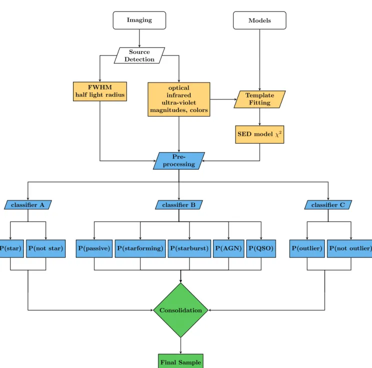
The CPz consists of three main stages shown in Fig.1. Stage I is the collection of the information on the flux and morphology of the sources and the subsequent photometric redshift estimation using template fitting. Stage II is the classification using three RFs to identify the A) probability of being a star, B) optimal photometric redshift setup and C) probability of being a pho-tometric redshift outlier, given the colors, χ2 _{values from the} template fitting step and morphology estimates (in our case the half-light radius). Finally, Stage III consists of the consolidation phase, during which a source is assigned a photometric redshift solution and i) probability to be a star, ii) probability for the red-shift to be wrong Eq. (8). We will describe the details behind each processing step by applying the method on the near-infrared VIKING and VIDEO Public VISTA Surveys cross matched with the CFHTLS, KiDS and SDSS optical surveys.

3.1. Stage I: catalogs and template fitting

Stage one of the CPz method consists of collecting information on the morphology (e.g., FWHM, half radius) and flux measure-ments and the spectral energy distribution (SED) model fitting. At this stage, allχ2_{estimates of the best fitting model per library} are saved and propagated into the pre-processing.

3.1.1. Photometric surveys

Modern extragalactic surveys profit from multiwavelength cov-erage from the ultra-violet to the mid-infrared, which allows for the estimation of good quality photometric redshifts. Future surveys for example with Euclid and LSST will provide

photometry from the u-band up to the H-band with

contin-uous coverage in wavelength. To test our method in com-parable conditions of Euclid plus LSST, we use the ESO

near-infrared Public VISTA surveys2 _{(Arnaboldi et al. 2007)} using the z,Y, J, H, and K photometric filters. We are using

both the VIKING (Jlim,AB=22.1, PI W. Sutherland) and VIDEO (J_lim,AB=24.5, PI M. Jarvis) surveys in order to benefit from the large area coverage and the depth, respectively. Euclid

observations will not have a K-band coverage, therefore we

will also discuss the impact of this particular filter on our results. The optical wavelength coverage (filtersu,g,r,i,z) is

from the SDSS survey (DR12,i_lim,AB=21.3,Alam et al. 2015), CFHTLS (T0007,ilim,AB=24.8,Hudelot et al. 2012) and KiDS (DR2,i_lim,AB=24.2,de Jong et al. 2015) surveys. We are also using mid-infrared observations in the W1 and W2 filters of

the WISE satellite (ALLWISE3_,W1

lim,AB=20.3, Wright et al.

2010; Mainzer et al. 2011) and ultra-violet (filters FUV, NUV) from the GALEX satellite (GR6/7, NUVlim,AB=20.5,

Morrissey et al. 2007). We corrected all photometric measure-ments according to the Schlegel maps of Galactic absorption (Schlegel et al. 1998) and the Cardelli law for the Milky way (Cardelli et al. 1989).

3.1.2. Spectroscopic surveys

We have selected spectroscopic redshift surveys which com-bined span a large redshift range (z∈[0−4]), represent all galaxy

types and include spectroscopically confirmed stars. These are

2 _{https://www.eso.org/sci/observing/PublicSurveys/}

sciencePublicSurveys.html

3 _{http://wise2.ipac.caltech.edu/docs/release/allwise/}

Imaging Source Detection Models optical infrared ultra-violet magnitudes, colors FWHM

half light radius Template

Fitting SED modelχ2 Pre-processing classifier B classifier A classifier C

P(star) P(not star) P(passive) P(starforming) P(starburst) P(AGN) P(QSO) P(outlier) P(not outlier)

Consolidation

Final Sample

Fig. 1.Components of the classification aided photometric redshift estimation method (CPz). Photometric and morphometric parameters are

extracted from the observed images. Magnitudes, colors and an estimation of the source shape (e.g., half light radius) make up the input attributes. The spectral energy distributions are fitted with model templates of star, galaxy and active galactic nuclei populations, theχ2 _{value of the best}

fitting model per library is added to the input attribute set. The pre-processing of the data consists of normalization and whitening of the attribute distributions (zero mean and variance of one) and the sample is split into training, testing and validation subsamples. The training sample is presented to three distinct classifiers, producing a probability for each source to A) be a star B) have an optimal photometric redshift from a collection of distinct libraries C) be a photometric redshift outlier. The final phase of CPz is the consolidation of the results, during which the test sample is used to decide on the thresholds adopted for each classifier and the assessment of the final accuracy on the classification and the photometric redshift performance using the validation sample.

SDSS4 _{(DR12 – 7.5×10}4_{sources,Alam et al. 2015), GAMA}5 (DR2 – 1.3×104 sources, Liske et al. 2015), VIPERS6 (DR1

– 3×103 sources, Garilli et al. 2014), VVDS (DR2– 3×103

4 _{http://www.sdss.org/dr12/data_access/bulk/} 5 _{http://www.gama-survey.org/dr2/data/cat/SpecCat/}

v08/

6 _{http://vipers.inaf.it/rel-pdr1.html}

sources, Le Fèvre et al. 2013), PRIMUS (DR1 – 2.7×104

sources,Coil et al. 2011;Cool et al. 2013), 6df (DR3 – 3×103

sources,Jones et al. 2004,2009). Some of these surveys provide a label, or comment introduced by visual inspection classify-ing the objects into star, galaxy, AGN or QSO. However, this labeling is neither homogeneous across all surveys, nor objec-tive. Thus, we keep this information for comparison with our machine-learning approach, but we do not use it during the training.

S. Fotopoulou and S. Paltani: CPz: Classification-aided photometric-redshift estimation Fotopoulou & Paltani: CPz

sources, Le Fèvre et al. 2013), PRIMUS (DR1 – 2.7×104 sources, Coil et al. 2011; Cool et al. 2013), 6df (DR3 – 3×103 sources, Jones et al. 2004, 2009). Some of these surveys pro-vide a label, or comment introduced by visual inspection classi-fying the objects into star, galaxy, AGN or QSO. However, this labeling is neither homogeneous across all surveys, nor objec-tive. Thus, we keep this information for comparison with our machine-learning approach, but we do not use it during the train-ing.

The sample used for this work consists exclusively of sources with the highest spectroscopic redshift quality7, matched to pho-tometric detections using a radius of 100_{. We use the following}

combination of wavelengths as quoted in the analysis and dis-cussion, namely: UV (filters FUV, NUV from GALEX), optical (filters u-z from any of SDSS, CFHTLS, KIDS), near infrared survey (filters z-K from any of VIKING, VIDEO), mid infrared (filters W1, W2 from WISE). Fig. 2 (a) shows the redshift dis-tribution per survey (colored lines) and the total galaxy sample (shaded gray area). The black spike located for demonstration purposes at -0.1 denotes the star sample. The panel (b) of the same figure shows the corresponding photometry for the spec-troscopic sample. SDSS photometry corresponds to 80% of the sample (∼200 deg2), while CFHTLS due to the extensive spec-troscopic follow of the W1 field (∼30 deg2) extends our sample to fainter magnitudes compared to SDSS.

We performed four CPz Runs using the following filter com-binations 1) u-K (∼7.8×104_{sources), 2) u-K – IR (∼5×10}4 sources), 3) UV – u - K (∼1.5×104sources) and 4) UV – u-K – IR (104_{sources) filters. This work does not address the impact} of missing values in the photometry, therefore each run is com-prised of sources that have good quality spectroscopic redshifts and photometric measurements in all filters. As the impact of the mid-infrared bands on the quality of the result is significant, we discuss in detail for the rest of the presentation of the method only Run u-K – IR. We differ the discussion of Runs one, three and four to Section 4.4.

3.1.3. Template fitting

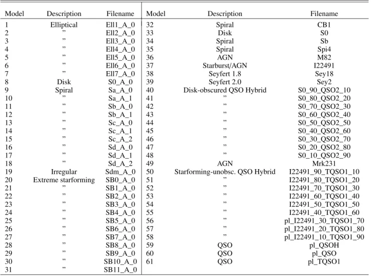
We performed SED fitting using the code LePhare8_{. We used the} template set selected for the COSMOS Survey (Scoville et al. 2007). The normal galaxy templates were introduced in Ilbert et al. (2009) and the AGN hybrid and QSO templates in Salvato et al. (2009). We used a redshift step of 0.01 from z=0 to z=6 for all models. The E(B-V) values used are 0.,0.05,0.1,0.15,0.2,0.3. The inclusion of emission lines, dust attenuation, absolute mag-nitude prior per library is reported in Table 4.

We also fit a model library of 154 stars (1150Å-25000Å) containing normal spectral types, F-K dwarfs and G-K giant components from the Pickles Atlas (Pickles 1998), white dwarfs (Bohlin et al. 1995) and subdwarf O and B stars (Bixler et al. 1991).

3.2. Stage II: classification

Stage two of CPz is the machine-learning classification, start-ing with the normalization transformations applied to the input attributes (pre-processing) created in Stage I. In the following section we discuss the setup of the classifiers. We are using

7 _{Sources denoted as stars and galaxies with zflag≥3 for GAMA and}

6dF, ZWARNING=0 for SDSS, and zflag=XX3 or XX4, X=0,1,2 for

VIPERS and VVDS. 8 _{www.cfht.hawaii.edu/~arnouts/lephare.html} 0 1 2 3 4 5 6 7 spectroscopic redshift 1 1 0 0 1 e 4 count GAMA 6 d f PRIMUS VIPERS SDSS VVDS stars (a) 0.0 0.5 1.0 1.5 2.0 2.5 3.0 3.5 4.0 redshift 10 12 14 16 18 20 22 24 i mag 0 2500 5000 7500 10000 0 1000 2000 (b)

Fig. 2.Spectroscopic redshift distribution of the u-k – IR sample used in this work. (a) The gray shaded area shows the total sample while the col-ored lines show the survey of origin. The black spike located for clarity at z=-0.1 shows the number of stars in the sample. (b) Magnitude dis-tribution for SDSS (red) and CFHTLS (blue) surveys comprising 80% and 20% of the galaxy sample respectively. The stars are shown with grey colour on this plot.

thescikit-learnimplementation in Python (Pedregosa et al., 2011) to pre-process and classify the data.

3.2.1. Input attributes and class definition

The attributes used for the classification are all color combi-nations and magnitudes of the photometric bands described in §3.1.1. For filtersutoKwe use both total (auto) magnitudes and 3” aperture magnitudes corrected to total, to account for flux lost due to the fixed size of the aperture. The correction is estimated Article number, page 5 of 20

Fig. 2.Spectroscopic redshift distribution of the u−k – IR sample used in this work.Panel a: gray shaded area shows the total sample while the colored lines show the survey of origin. The black spike located for clarity atz=−0.1 shows the number of stars in the sample. Panel b: magnitude distribution for SDSS (red) and CFHTLS (blue) sur-veys comprising 80% and 20% of the galaxy sample respectively. The stars are shown with grey colour on this plot.

The sample used for this work consists exclusively of sources with the highest spectroscopic redshift quality7_{, matched to} pho-tometric detections using a radius of 100_{. We use the following}

combination of wavelengths as quoted in the analysis and dis-cussion, namely: UV (filters FUV, NUV from GALEX), optical (filtersu−zfrom any of SDSS, CFHTLS, KIDS), near infrared

survey (filtersz−Kfrom any of VIKING, VIDEO), mid infrared

7 _{Sources denoted as stars and galaxies with zflag≥3 for GAMA and}

6dF, ZWARNING=0 for SDSS, and zflag=XX3 or XX4, X=0,1,2 for

VIPERS and VVDS.

(filtersW1,W2from WISE). Figure2a shows the redshift

dis-tribution per survey (colored lines) and the total galaxy sample (shaded gray area). The black spike located for demonstration purposes at −0.1 denotes the star sample. The panel b of the

same figure shows the corresponding photometry for the spec-troscopic sample. SDSS photometry corresponds to 80% of the sample (∼200 deg2), while CFHTLS due to the extensive

spec-troscopic follow of theW1field (∼30 deg2) extends our sample

to fainter magnitudes compared to SDSS.

We performed four CPz Runs using the following filter com-binations 1)u−K(∼7.8×104sources), 2)u−K– IR (∼5×104

sources), 3) UV–u−K(∼1.5×104sources) and 4) UV–u−K–

IR (104_{sources) filters. This work does not address the impact} of missing values in the photometry, therefore each run is com-prised of sources that have good quality spectroscopic redshifts and photometric measurements in all filters. As the impact of the mid-infrared bands on the quality of the result is significant, we discuss in detail for the rest of the presentation of the method only Runu−K– IR. We differ the discussion of Runs one, three

and four to Sect.4.4. 3.1.3. Template fitting

We performed SED fitting using the code LePhare8_{. We} used the template set selected for the COSMOS Survey (Scoville et al. 2007). The normal galaxy templates were intro-duced inIlbert et al.(2009) and the AGN hybrid and QSO tem-plates inSalvato et al. (2009). We used a redshift step of 0.01 fromz =0 toz= 6 for all models. TheE(B−V) values used

are 0,0.05,0.1,0.15,0.2,0.3. The inclusion of emission lines, dust attenuation, absolute magnitude prior per library is reported in Table4.

We also fit a model library of 154 stars (1150 Å–25 000 Å) containing normal spectral types, F-K dwarfs and G-K giant components from the Pickles Atlas (Pickles 1998), white dwarfs (Bohlin et al. 1995) and subdwarf O and B stars (Bixler et al. 1991).

3.2. Stage II: classification

Stage two of CPz is the machine-learning classification, start-ing with the normalization transformations applied to the input attributes (pre-processing) created in Stage I. In the following section we discuss the setup of the classifiers. We are using

thescikit-learnimplementation in Python (Pedregosa et al.

2011) to pre-process and classify the data. 3.2.1. Input attributes and class definition

The attributes used for the classification are all color combi-nations and magnitudes of the photometric bands described in Sect. 3.1.1. For filters u toK we use both total (auto)

magni-tudes and 300_{aperture magnitudes corrected to total, to account}

for flux lost due to the fixed size of the aperture. The correction is estimated on point-like sources and applied to the entire cata-log. Particularly for theW1andW2WISE bands, we are using

only the total magnitudes since the PSF of WISE is much larger compared to the optical and near-infrared bands (∼600_compared

to 0.800_–1.300 _{respectively). As a proxy for the morphology, we}

are using the half light radius estimated for the bands g up to K, defined as the radius up to which 50% of the total flux is

enclosed. For point-like sources (stars and QSO) this radius will

8 _{www.cfht.hawaii.edu/~arnouts/lephare.html}

Table 1.Models used during the photometric redshift estimation with template fitting.

Model Description Filename Model Description Filename

1 Elliptical Ell1_A_0 32 Spiral CB1

2 ” Ell2_A_0 33 Disk S0

3 ” Ell3_A_0 34 Spiral Sb

4 ” Ell4_A_0 35 Spiral Spi4

5 ” Ell5_A_0 36 AGN M82

6 ” Ell6_A_0 37 Starburst/AGN I22491

7 ” Ell7_A_0 38 Seyfert 1.8 Sey18

8 Disk S0_A_0 39 Seyfert 2.0 Sey2

9 Spiral Sa_A_0 40 Disk-obscured QSO Hybrid S0_90_QSO2_10

10 ” Sa_A_1 41 ” S0_80_QSO2_20 11 ” Sb_A_0 42 ” S0_70_QSO2_30 12 ” Sb_A_1 43 ” S0_60_QSO2_40 13 ” Sc_A_0 44 ” S0_50_QSO2_50 14 ” Sc_A_1 45 ” S0_40_QSO2_60 15 ” Sc_A_2 46 ” S0_30_QSO2_70 16 ” Sd_A_0 47 ” S0_20_QSO2_80 17 ” Sd_A_1 48 ” S0_10_QSO2_90 18 ” Sd_A_2 49 AGN Mrk231

19 Irregular Sdm_A_0 50 Starforming-unobsc. QSO Hybrid I22491_90_TQSO1_10

20 Extreme starforming SB0_A_0 51 ” I22491_80_TQSO1_20

21 ” SB1_A_0 52 ” I22491_70_TQSO1_30 22 ” SB2_A_0 53 ” I22491_60_TQSO1_40 23 ” SB3_A_0 54 ” I22491_50_TQSO1_50 24 ” SB4_A_0 55 ” I22491_40_TQSO1_60 25 ” SB5_A_0 56 ” pl_I22491_30_TQSO1_70 26 ” SB6_A_0 57 ” pl_I22491_20_TQSO1_80 27 ” SB7_A_0 58 ” pl_I22491_10_TQSO1_90

28 ” SB8_A_0 59 QSO pl_QSOH

29 ” SB9_A_0 60 QSO pl_QSO

30 ” SB10_A_0 61 QSO pl_TQSO1

31 ” SB11_A_0

Notes.Left hand side: normal galaxy models. The starformation increases from top to bottom (seeIlbert et al. 2009for more details). Right hand

side: normal, AGN-QSO and hybrid models. The AGN fraction varies from 0–100% as noted in the name of the model, e.g. S0_90_QSO2_10 is a combination of 90% flux from a disk galaxy and 10% flux contribution from an obscured QSO. The prefix “pl_” denotes that the model has been extended to the ultra-violet assuming a power-law (seeSalvato et al. 2009for a detailed description).

be very close to the FWHM of the PSF, while for extended objects it is significantly larger. Additionally, we are using the values of the χ2 _{for the star models in classifier A (star} classi-fier) and the values of theχ2 _{of galaxies, AGN, QSO one for} each corresponding library setup for classifier B (galaxy classi-fier). The total number of input attributes is 263.

The definition of the target classes is of paramount impor-tance for supervised machine-learning. With our method we aim to train three classifiers, thus we need three labels for each object. Namely, we create a star classifier (classifier A), a galaxy classifier tuned to return the class for which the photometric red-shift solution is optimal (classifier B) and a classifier to identify photometric redshift outliers (classifier C). Even though techni-cally possible, we do not combine all categories into one classi-fier. We opt for a flexible scheme within which we have the best photometric redshift estimation for all sources and impose only during the consolidation phase probability thresholds to identify stars and outliers. With this approach, we can tune during the consolidation phase the completeness and purity as desired for each specific science application.

The star – no star label is assigned using a sample of spec-troscopically confirmed stars, used to train classifier A. The galaxy class label is tuned to identify the optimal photometric

redshift class. It is assigned according to the minimum value of∆zi = |zphoti−zspec|, wherei corresponds to the library con-figurations given in Table4. Thus, Classifier B will recognize, for example for Case III, which of the five classes (passive, starforming, starburst, AGN, QSO) will provide the best photo-metric redshift estimate compared to the available spectroscopic value. Finally, if |z_photi−z_spec|/(1+z_spec)>0.15 for all

photo-metric redshift classes, the solution is considered a catastrophic outlier and is used as training in Classifier C. The catastrophic outliers will thus contain stars, QSOs – notoriously difficult to model due to their featureless SEDs – and rare galaxies (e.g., extreme obscured or extremely starforming) that are not repre-sented by our template selection.

3.2.2. Pre-processing: whitening and normalization

There are two main operations that must take place before the data can be presented to the classifier, collectively called pre-processing. These operations are the treatment of missing values, also called data imputation and the whitening and normalization of the dataset.

A typical approach in machine-learning when it comes to the treatment of missing values is the substitution of the value

S. Fotopoulou and S. Paltani: CPz: Classification-aided photometric-redshift estimation with the mean of the distribution. The mean of the distribution

is the preferred substitution in the case of lacking observational data and this is the approach we adopt for this work. However, in an astronomical context other data imputation methods could be considered. For example, it can be that a source has an upper limit (non-detection), lower limit (saturation), or missing value (not observed). The impact of the data imputation depends on the specifics of each dataset, taking into account the sky cov-erage of the observations, including the tiling of the observa-tions and any masking due to bright stars and the depth of the photometry.

Whitening and normalization are transformations that cen-ter the distribution of the input attributes around zero and make the distribution of the values have a standard deviation of one. Machine-learning algorithms require whitening and normaliza-tion of the data to avoid recogninormaliza-tion of artificial structures in the data due to difference in the order of magnitude of the attribute values, for example by mixing flux and magnitude estimates. It is critical that the same transformation applied to the training sample must be applied to the test and validation samples.

3.2.3. Train–test–validation samples

We split our sample of about 50 000 sources into three subsam-ples with ratio 1:1:1 for training, testing and validation. It is important that all three samples are representative of each other, therefore we first sort according to redshift and then split the sample taking every third source for each of the classifiers under consideration. During the training phase, the algorithm creates the Random Forest that maps best the input attributes to the target classes. After the training is complete and the forest is fully grown, we use the test sample that was not part of the training sam-ple to estimate the accuracy of the classifier and identify the appro-priate thresholds to adopt to separate stars and outliers. Finally, after all optimizations are performed, we estimate the final qual-ity of CPz method using the validation sample which is never seen by the classifier during the training and testing phases. If not enough data are available for a separate validation set, it is common practice to perform cross-validation. During this proce-dure a handful of data are purposely left aside during the train-ing and the classifier accuracy is tested on them. If this proce-dure is performedn-times, we refer ton-fold cross-validation. We

have verified that with three-fold cross-validation we obtain simi-lar accuracy results to the ones estimated with a dedicated testing sample.

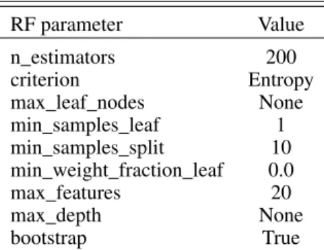
A number of parameters are available to tune the perfor-mance of the Random Forest algorithm. We performed a grid search using three-fold cross validation in the training phase to select the best parameters for our work given in Table 2. The parameter n_estimators is the number of trees created. As a rule of thumb, the higher the number the more accurate the classifi-cation, however there is a limit after which the accuracy does not increase noticeably with an increasing expense on the computing time. In our case we found that 200 trees was a good trade-off between accuracy and computing time. The rest of the param-eters in Table2control the split of the input attributes and the creation of the trees.

3.2.4. Classifier A: is it a star or not?

First we examine the separation between stars and galaxies. We achieve accuracy of ACC=99.7%, precisionP=99.1%, recall R = 99% and fall-out of only F = 0.2%. As the locus

occu-Table 2.Random Forest set-up parameters.

RF parameter Value n_estimators 200 criterion Entropy max_leaf_nodes None min_samples_leaf 1 min_samples_split 10 min_weight_fraction_leaf 0.0 max_features 20 max_depth None bootstrap True

Notes.The parameter n_estimators is the number of trees created.

pied by stars in color space is narrow and almost disjoint to that of galaxies, it is an easier classification problem especially if infrared data are available. In Fig.3a we plot the results of the test sample. The color plot (Y −W1) vs (g−J) shows clearly

the separation in color space between stars (black), selected as sources with Pr[star]>50% and galaxies (gray). Similar plots using IRAC colors have been used previously in the literature (e.g.,Ilbert et al. 2009).

By default, the Random Forest implementation in Python will assign each object to the class with the highest probabil-ity. In the case of two categories the threshold is set at 50%. Nevertheless, given the science interest, a selection of pure or complete sample might be of interest. Since the Random For-est provides also as output the probability for each class, it is possible to select the sample according to the desired specifica-tions. Panel b of Fig. 3shows the level of completeness (gray dot-dashed line) and purity (black line) as a function of proba-bility threshold. For example, a threshold P[star]>80% would lead to roughly 100% purity and 95% completeness.

The last panel of Fig.3visualizes the performance of clas-sifier A in a confusion matrix. The diagonal elements repre-sent the percentage of true positive classifications, while the off-diagonal elements show the percentage of false positive clas-sifications. A perfect classifier will have black diagonal elements and white off-diagonal elements, classifier A with ACC=99.7% shows excellent performance.

3.2.5. Classifier B: which is the best photo-zlibrary?

Classifier B is trained to identify the model library that will pro-vide the optimal photometric redshift solution judged by the best photometric redshift. As discussed in Sect. 3.2.1, we grouped the galaxy models roughly according to their star-formation into passive, starforming and extreme starforming which for short we will refer to as starburst. We have also included two additional libraries: AGN and QSO (see Table 1 for the full list of templates used and Sect. 4.1 for the explored galaxy class combinations). In Fig. 4 we show the objects identified in the test sample in each category using the same color-color plot as in Fig. 3. The gray points show all of the sample for comparison. We note that classifier B is applied to the full sample without any a priori knowledge of stars. Passive and starforming galaxies trace a somewhat different region in the color space, albeit with a large overlap in this two-dimensional representation. QSOs on the other hand shown in panel e are very well isolated with respect to the normal galaxy popula-tion. Finally, as expected, the AGN population is located in the overlap region between the normal galaxies and the QSO, A14, page 7 of19

2 0 2 4 6 8 g-J 3 2 1 0 1 2 3 Y-W1 0 20 40 60 80 100 probability threshold 0 20 40 60 80 100 quality level (%) completeness purity star _galaxy Predicted label star galaxy True label 0.1 0.2 0.3 0.4 0.5 0.6 0.7 0.8 0.9 (a) (b) (c)

Fig. 3.Stars identified in the test sample.Panel a: color locus occupied by the stars (black points) compared to the color locus occupied by the non-stars, i.e. galaxies and AGN (gray points) adopting a probability threshold of 50%.Panel b: completeness (gray dot-dashed line) and purity (black solid line) of the identified star sample for each given probability threshold given on thex-axis.Panel c: summary of the performance of the classifier in a confusion matrix.

Fig. 4.Output of the galaxy classification (colored points) compared to the total input population (gray points). The galaxy class is given below

each plot. We note that stars have not been excluded a priori.

since by construction their SEDs are a mixture of the two components.

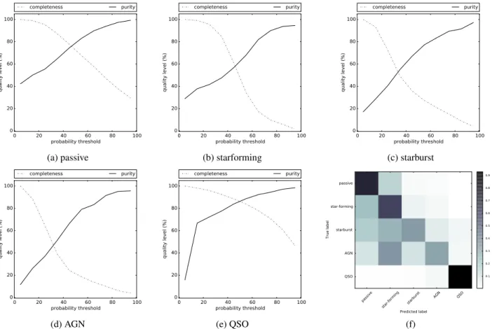
The weighted average accuracy of classifier B over all classes is about 64%. Since in this case we have a multiclass classification, the average accuracy is not as informative. In Fig.5we show the completeness and purity per galaxy category as a function of probability threshold, similarly to Fig.3. The minimum threshold for class assignment is 20%. As seen from

panels a–e such a threshold would correspond to complete (70%–90%) but rather impure samples (30%–60% purity). We note that in the final galaxy sample the performance will be slightly better since for now the stars are still included in the sample. The confusion matrix in the last panel of Fig. 3 shows the relative mixing of the classes adopting the default class assignment. The QSOs are well separated from all other classes and with little false positive detections. The same is

S. Fotopoulou and S. Paltani: CPz: Classification-aided photometric-redshift estimation 0 20 40 60 80 100 probability threshold 0 20 40 60 80 100 quality level (%) completeness purity 0 20 40 60 80 100 probability threshold 0 20 40 60 80 100 quality level (%) completeness purity 0 20 40 60 80 100 probability threshold 0 20 40 60 80 100 quality level (%) completeness purity

(a) passive (b) starforming (c) starburst

0 20 40 60 80 100 probability threshold 0 20 40 60 80 100 quality level (%) completeness purity 0 20 40 60 80 100 probability threshold 0 20 40 60 80 100 quality level (%) completeness purity passive star-forming starburst AGN QSO Predicted label passive star-forming starburst AGN QSO True label 0.1 0.2 0.3 0.4 0.5 0.6 0.7 0.8 0.9

(d) AGN (e) QSO (f)

Fig. 5.Completeness (dashed line) and purity (solid line) of each galaxy class as a function of probability threshold.Panel f: confusion matrix. true, but with lesser quality for the passive galaxies. The

largest mixing is present between the starforming and the AGN population.

Since in our sample we know the true classification between stars and galaxies, it is interesting to explore the confusion between these two classes as revealed in Fig.4. The sample of spectroscopically confirmed stars (∼2500 sources) is distributed

in four galaxy classes: passive (71%), starforming (3%), star-burst (16%), and AGN (10%). No stars were classified as QSO. Nevertheless, 74% of the star sample is placed atz=0 from the

SED fitting. Stars can mimic passive galaxies are redshift zero (99% of passive sample, 57% of total star sample). Stars classi-fied as starforming and starburst galaxies are placed either at red-shift zero (64%) with varying amounts of absorption, or at higher redshifts (0.01<z<1.0) with the SED fitting selecting the

tem-plate with the highest allowed absorption (E(B−V)=0.3).

Sim-ilarly, 51% of the stars classified as AGN are placed atz = 0,

with varying amounts of E(B−V) depending on the template

SED. In the AGN case, the dominant template that is the best fit to stars at non-zero redshifts is template 48 consisting of 10% S0 non-starforming disk galaxy and 90% of QSO2, which is a tem-plate with intrinsic heavy obscuration in the UV-optical part of the spectrum. If we use the results of classifier A to remove the stars from the galaxy sample the weighted classification accu-racy is not affected significantly (worsens about 4%), since the stars are classified with high accuracy (weighted average 85%) even using in Classifier B9_.

9 _{This means that 85% of the star sample is distributed accurately to the}

input classes that originally have “star-like” SEDs. Incidentally, 60% of the star sample is correctly placed atz=0 from fitting their SEDs with galaxy templates only.

3.2.6. Classifier C: is the photo-zsolution acceptable? Outlier identification is a difficult task, because there are many reasons that can lead to a failed estimation of photometric red-shift. The reasons include intrinsic physical properties such as i) variability, as shown in Salvato et al. (2009), ii) rare or not represented SED in the template library and iii) true degenera-cies in color space (Richards et al. 2001). External factors can also lead to a failed photometric redshift estimation i) bad pho-tometry, for example saturation ii) source misassociation, for example blending due to large PSF or astrometric offsets iii) wrong spectroscopic redshift.

We explored the possibility to identify outliers using a ran-dom forest classifier. The sample used contains the sources that follow Eq. (8). In Fig.6 we show, similarly to the stars, the output classification of the test sample. The black points correspond to the sources with P[outlier]>50%. We see that the majority of the outliers is gathered in the locus occu-pied by QSO and stars.The average accuracy of Classifier C is 97.9%, this score is also immune to the presence of stars (see Sect.3.2.5) as the stars are classified as outliers with very high accuracy (99%).

Similarly to classifiers A and B, adopting a more conser-vative outlier threshold, will allow for a more complete sam-ple, P[outlier]>20% leads to 80% complete sample in the expense of purity (40%). However, the selection threshold can be adjusted according to the science case, or even ignored alto-gether. Examining the confusion matrix in the last panel of Fig.6 we see that there are many false positive identifications of good photometric redshift estimations as outliers (60%) at P[outlier]>50%, however most outliers are indeed classified as outliers.

2 0 2 4 6 8 g-J 3 2 1 0 1 2 3 Y-W1 0 20 40 60 80 100 probability threshold 0 20 40 60 80 100 quality level (%) completeness purity outlier not outlier Predicted label outlier not outlier True label 0.1 0.2 0.3 0.4 0.5 0.6 0.7 0.8 0.9 (a) (b) (c)

Fig. 6.Same as Fig.3but for classifier C.

Table 3.Number of sources and photometric redshift performance after (A) class assignment according to the highest probability and/or star and

outlier rejection (B) class assignment according to the highest probability but imposing a probability threshold for all galaxy classes.

Rej. type Consolidation A Consolidation B

N % σ η(%) N % σ η(%)

No rejection 16 394 100.0 0.035 4.9 13 773 84.0 0.032 4.5

Star 13 859 84.5 0.042 4.2 11 294 68.9 0.040 3.7

Outlier 15 752 96.1 0.033 2.6 13 212 80.6 0.030 2.1

Star & outlier 13 436 82.0 0.041 2.9 10 937 66.7 0.039 2.3

3.3. Stage III: consolidation

By creating three classifiers to provide a star, galaxy and out-lier classification we have flexibility in the consolidation phase. Here, the scientific goal of the survey can be taken into account in adopting the appropriate probability threshold selection for each classifier, using the results of the test sample presented in Sects.3.2.4–3.2.6.

3.3.1. Threshold selection

For classifier B, we have performed multiclass classification and the sum of the probabilities of the five classes is equal to unity. In this case, the default RF behavior assigns as best class the one with the highest probability (Consolidation A). However, we may also choose to make an extra threshold cut for the galaxy classes (Consolidation B). Here we adopt the threshold of 40% for all normal galaxy classes and AGN, corresponding to at least 50% pure samples and the default 20% threshold for QSO. In Table 3 we show the photometric redshift quality for the two cases. We notice a slight improvement in the overall photometric performance, both in terms of accuracy (σ_A=0.035,σ_A=0.032) and percentage of outliers (ηA = 4.9%−η_A = 4.5%) to the

expense of the numbers of available sources with 84% of the original sample retained after consolidation B.

3.3.2. Rejection of stars and outliers

In addition, we can select the threshold of the star and/or out-lier identification. For the star labeling we adopt P[star]>50% corresponding to about 99% completeness and accuracy. Respectively for the outlier rejection we opt for completeness

over purity adopting a threshold of P[outlier]>20% which cor-responds to about 70% completeness and 40% purity. Table3 shows the performance of the photometric redshift estimation and the corresponding number of sources remaining the sample for each rejection step. We note that in general, rejection of stars and outliers will lead to higher accuracy and less outliers both when adopting the highest galaxy class probability (consolida-tion A) and when imposing an absolute threshold (consolida(consolida-tion B) compared to no rejection at all. Seemingly the accuracy of photo-zworsens when stars are rejected (fromσno rej = 0.035 toσ_{star rej} =0.042). This is due to the fact that the majority of the stars are placed correctly at redshift zero during SED fitting, even when using galaxy templates (60% of the star sample, see Sect.3.2.5).

3.3.3. Rejection of uninformative PDFs

Template fitting algorithms, in our case specifically LePhare, pro-vide as an output the full probability distribution function (PDF) for the photometric redshift estimate. Figure7shows a selection of PDFs ranging from very narrow to multimodal to very broad PDFs normalized to unity at the peak of the distribution for demon-stration purposes. The solid lines show the photometric redshift assignment, while the dashed lines show the spectroscopic red-shift value. The first panel of the first row shows an example of a very good photo-zestimation, where the PDF is narrow and

centered on the true redshift value. The second panel of the first row shows an equally narrow solution, but centered on the wrong value. The second and third rows show PDFs that are broad and/or multimodal but still include the true redshift solution.

It is possible to rank the PDFs according to the informa-tion gained compared to a flat distribuinforma-tion by means of the

S. Fotopoulou and S. Paltani: CPz: Classification-aided photometric-redshift estimation 0.0 0.5 1.0 1.5 2.0 2.5 3.0 3.5 4.0 redshift 0.0 0.2 0.4 0.6 0.8 1.0 P D F z-spec z-phot 0.0 0.5 1.0 1.5 2.0 2.5 3.0 3.5 4.0 redshift 0.0 0.2 0.40.6 0.8 1.0 P D F z-spec z-phot 0.0 0.5 1.0 1.5 2.0 2.5 3.0 3.5 4.0 redshift 0.0 0.2 0.4 0.6 0.8 1.0 P D F z-spec z-phot 0.0 0.5 1.0 1.5 2.0 2.5 3.0 3.5 4.0 redshift 0.0 0.2 0.40.6 0.8 1.0 P D F z-spec z-phot 0.0 0.5 1.0 1.5 2.0 2.5 3.0 3.5 4.0 redshift 0.0 0.2 0.4 0.6 0.8 1.0 P D F z-spec z-phot 0.0 0.5 1.0 1.5 2.0 2.5 3.0 3.5 4.0 redshift 0.0 0.2 0.40.6 0.8 1.0 P D F z-spec z-phot

Fig. 7.Example probability distribution functions (PDF) from the consolidated sample.First row: two sources with high information content, DKL∼7.Second row: broader and multimodal PDFs withDKL∼4, while thelast rowshows the PDFs with the least information contentDKL<2.

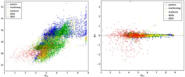
1 2 3 4 5 6 7 8 9 DKL 12 14 16 18 20 22 J passive starfoming starburst AGN QSO 1 2 3 4 5 6 7 8 9 DKL ¡3 ¡2 ¡1 0 1 2 3 ¢ z passive starforming starburst AGN QSO

Fig. 8.Left:Y-band magnitude vs the Kullback–Leibler divergence,DKL. The PDF of brighter sources carries more information content, i.e.

narrower PDF, compared to faint sources.Right:∆z=zphot−zspecas a function of information content split per galaxy class. QSO PDFs have the

distinctly lower information content compare to normal galaxies and AGN. Kullback–Leibler divergence (Kullback & Leibler 1951):

DKL(P||Q)= Z +∞

−∞

p(x) log₂ p(x)

q(x)dx, (9)

where P and Q are two continuous random variables and p, q their corresponding probability density functions. The D_KL

divergence, a useful diagnostic of information theory, has been used in the literature for quantifying the information gain for example, when performing bayesian analysis of X-ray spectra (Buchner et al. 2014) and when modeling the 5−10 keV AGN

luminosity function (Fotopoulou et al. 2016a). Further informa-tion can be found inBishop(2006).

Here we consider as P the photometric redshift PDF and asQ

the extremely agnostic case in which we only know that a source must be between redshift zero and six, assuming a flat distribu-tion. The information gain is measured in bits since the logarithm

with base 2 is used10_{. In Fig.8a we show the trend between the}

DKL and the J band magnitude. As expected, brighter sources

(J<20) tend to have higherD_KLvalues signifying that the PDF

carries more information with respect to a flat distribution, thus signifying a narrow PDF. As we move to fainter objects, theD_KL

is also reduced to lower values reflecting the difficulty of con-straining the PDF of a faint object. The same trends hold for all photometric bands. However, we do note a small cloud of sources withDKL<2. These are sources with broad PDFs simi-lar to the bottom row of Fig.7. On the other end, we find sources with the highest DKL values, aggregated at DKL ∼ 8.7. These correspond to sources withz_phot = 0.0−0.01 with very narrow

PDFs, a telling sign of failed photo-z, most of the time due to

noisy photometry.

10 _{One bit corresponds to the reduction of the standard deviation of a}

Gaussian distribution by a factor of three.

0

1

2

3

4

5

z

spec

0

1

2

3

4

5

z

ph

ot

0

5

10

15

20

25

probability mass

0.0 0.5 1.0 1.5 2.0 2.5 3.0 3.5 4.0

redshift

0

500

1000

1500

2000

2500

count

Fig. 9. Left: histogram of stacked PDFs of the final sample. The solid line shows the diagonal, the dashed and dotted lines mark the |zphot−zspec|/(1+zspec) =0.05,0.15 respectively. The red dots show the point estimate of the photometric redshifts, here the mode of the PDF. Right: comparison of the photometric (red) and spectroscopic (black) redshift distributions.

It is also instructive to examine the D_KL values according

to the galaxy classes as determined with classifier B. Panel b of Fig.8shows the difference∆z=z_phot−z_specas a function of

the DKL. The color coding corresponds to the five classes con-sidered here as given in the legend. Most notably, there is no clear-cutDKLthat can be used to identify good PDFs. However, we note that the QSO class has systematically lowerD_KLvalues

compared to the normal galaxies and also that the AGNs show similar values as the normal galaxies. This is explained by the discriminating features present in galaxy and AGN SEDs (e.g., Balmer break) contrary to QSO SEDs which are mostly feature-less power-laws hence leading to feature-less constrained photometric redshift solutions.

3.3.4. Final sample

Gathering all information from the previous sections, we select as our final sample the configuration of consolidation B (absolute probability threshold of 40% for normal galaxies and AGN, 20% for QSO), imposing rejection of stars (P[star]<50%) and

out-liers (P[outlier]>20%) and rejecting sources that have either too

narrow or too broad PDFs (DKL<2 orDKL>8.5, 282 sources, 3% of the sample). The final validation sample consists of 10.655 objects with photometric redshift accuracyσNMAD=0.039 with 2.3% outliers.

On the left hand side of Fig.9we show the photometric red-shift versus the spectroscopic redred-shift. The red dots show the mode of the PDF, adopted as point-estimate representation of the photometric redshift estimation. The solid red line is the diagonal while the dashed and dotted lines show the region of

|zphot−zspec|/(1+zspec)=0.05,0.15 respectively. The gray scale shows the 2D histogram of the stacked PDFs binned at resolu-tion ∆z=0.1. The gray scale shows the amount of probability

per cell. The black-colored cells show regions containing more than 25% of the probability mass. The right hand side of the same Figure shows the redshift distribution of the photometric redshift point estimates compared to the spectroscopic redshift values.

4. Discussion 4.1. Galaxy classes

In order to identify the optimal photometric redshift libraries, we test four model library setups as shown in Table4. For this com-parison we use the validation sample with photometric bands from theu-band to theW2filter.

In Case 0 we include all galaxy and AGN models in a sin-gle library. This is done to test the discriminating power of

χ2_{. Case 0 is the least optimal photometric redshift} estima-tion, since the AGN and QSO are not treated in a special way and emission lines are not present in the templates (σ = 0.06,

η=9.2%). However, it has been used previously in the literature mostly by including one or two QSO templates within a galaxy library.

Case I resembles the set-up that was adopted by the COS-MOS team as described inIlbert et al.(2009) andSalvato et al. (2009, 2011). This set-up was originally created to optimize the photometric redshift of galaxies and X-ray detected AGN. Briefly, X-ray detected sources are confronted with QSO and AGN hybrid models to account for the combined emission from the QSO and the host galaxy. The templates are empirical and hence they include observed emission lines. The EXTNV and QSOV model libraries consist of the same templates (No. 32– 61 of Table1) with the application of differentB-band absolute

magnitude priors: −24<MB<−8 for strong AGNs (extended and not varying sources withFx >8×10−15erg s−1cm−2) and

−30<M_B<−20 for QSO dominated objects (optical

point-like or varying sources). These AGN templates span a range in AGN – host galaxy combinations ranging from non-active (e.g., CB1, S0) to pure QSO templates (e.g., pl_QSO, pl_QSOH, pl_TQSO1). Salvato et al. (2009) selected these templates as the best representation of the active galaxy population in the COSMOS survey. The remaining sources that are either not X-ray detected or are X-ray detected but appear extended in the optical, are not varying and have Fx < 8×10−15erg s−1cm−2

are fitted using normal galaxy models and luminosity prior of

S. Fotopoulou and S. Paltani: CPz: Classification-aided photometric-redshift estimation

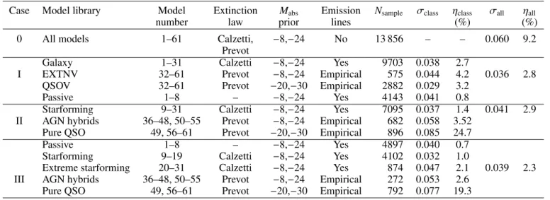
Table 4.Template fitting class set-up and respective performances.

Case Model library Model Extinction M_abs Emission N_sample σ_class η_class σ_all η_all

number law prior lines (%) (%)

0 All models 1–61 Calzetti, −8,−24 No 13 856 – – 0.060 9.2

Prevot

Galaxy 1–31 Calzetti −8,−24 Yes 9703 0.038 2.7

I EXTNV 32–61 Prevot −8,−24 Empirical 575 0.044 4.2 0.036 2.8

QSOV 32–61 Prevot −20,−30 Empirical 2882 0.029 3.2

Passive 1–8 – −8,−24 Yes 4143 0.041 0.8

Starforming 9–31 Calzetti −8,−24 Yes 7095 0.037 1.4 0.041 2.9

II AGN hybrids 36–48, 50–55 Prevot −8,−24 Empirical 682 0.058 3.52

Pure QSO 49, 56–61 Prevot −20,−30 Empirical 896 0.085 24.7

Passive 1–8 – −8,−24 Yes 4897 0.040 0.7

Starforming 9–19 Calzetti −8,−24 Yes 4102 0.032 1.0

Extreme starforming 20–31 Calzetti −8,−24 Yes 874 0.047 2.1 0.039 2.3

III AGN hybrids 36–48, 50–55 Prevot −8,−24 Empirical 272 0.053 2.6

Pure QSO 49, 56–61 Prevot −20,−30 Empirical 792 0.077 19.3

Notes.The numbers quoted in this table include star and outlier rejection.

This method has been successfully applied to other fields such as the Lockman Hole (Fotopoulou et al. 2012), theChandra

Deep Field South (Hsu et al. 2014) and AEGIS-X (Nandra et al. 2015) and it is the current state of the art, used when X-ray data are available for the whole field in consideration. However, the correct implementation of the method requires splitting the sample into point-like and varying sources and also having an estimate of X-ray flux. This information is not available homo-geneously across our sample, therefore we cannot test the result of a COSMOS-like approach directly for this sample. Instead, we used the optimal library set-up identified for the COSMOS field inSalvato et al.(2011) and use a machine-learning classi-fier to identify which objects are best fitted for each of the three classes. We find that this library setup shows very good perfor-mance both in terms of accuracy (σ =0.035) and catastrophic outliers (η =2.8%), achieving an improvement over Case 0 by factor of two on the accuracy and by a factor of three on the fraction of outliers.

Case II is an extension of the previous set up with two main differences. We divide the normal galaxy library into pas-sive (No. 1–8 models in Table1) and starforming systems (No. 9–31 models) and we use the hybrid AGN models (No. 36– 48 and 50–55, AGN hybrids library) separately from the pure QSO models (No. 49, 56–61, pure QSO library) for a total of four model libraries. We have applied the correspondingB-band

luminosity prior of −24<M_B<−8 for normal galaxies and

AGN and −30<MB<−20 for QSO. We find that this setup

represents a significant improvement over Case 0 and slightly under-performs compared to Case I (σ_II=0.04,η=2.9%).

Finally, Case III is similar to Case II with the extra sep-aration between starforming (No. 9–19 models) and extreme-starforming galaxies (which we refer to as starburst for short, No. 20–31 models). We see that Case III shows better perfor-mance compared to all previous cases in terms of catastrophic outliers (η = 2.3%) and achieves slightly worse performance compared to Case I in terms of accuracy (σ = 0.039). We can examine further the accuracy per galaxy class, also given in Table 4, keeping in mind that each class contains a dif-ferent collection of models and a difdif-ferent galaxy population chosen by the machine-learning classification. The performances resemble the expectation for each population, namely passive

and spiral galaxies have SEDs reach in discriminating features that can be identified through model fitting showingσ ∼ 0.04

and 0.5–1.0% fraction of catastrophic outliers. The degenera-cies present in the starburst and AGN colors creates a higher fraction of catastrophic outliers (2–3%), however the accuracy remains very good and close to the passive and spiral galax-ies (σ ∼ 0.04−0.05). Lastly, as expected the QSO

popula-tion shows the least optimal photometric redshift performance (σ =0.07 andη =20%), mostly due to their featureless SEDs which is particularly problematic when using only broadband photometry.

It is evident that the simple inclusion of AGN templates in a galaxy library leads to the worst performance (Case 0). We recover the good behavior of the setup ofSalvato et al. (2009, 2011), where the split between galaxies and AGN leads to an improvement higher than a factor of two both on accuracy and outlier rate compared to Case 0. More interestingly, the fur-ther separation of the galaxy library and the consideration of pure AGN and QSO libraries is beneficial when we opt for pure classes of objects, for example, separating the starform-ing and starburst galaxies in two distinct classes and AGN from QSO, reducing the outlier rate and while maintaining compara-ble accuracy.

4.2. Feature Importance

One of the attractive features of Random Forest is the relative ranking of the discriminating power of the input attributes. In Table5we list the top 10 most important features identified by the Random Forest for each of our three classifiers. The subscript 3 refers to magnitudes estimated within 300 _{aperture diameter.}

For Classifier A, the star-galaxy separator, the infrared colors carry the dominant discriminating power, especially the WISE bands. The top three most important features are the colors

J3−W1,Y3−W1, J3−W2. The colors identified by the

Ran-dom Forest correspond to the color-color plots presented in this paper and also found in similar forms with the literature.

The clear separation between the star and galaxy population as seen in Fig.3, at least for the population withg−J>2 leaves

little ambiguity. However, the population with g−J<2 is a

locus occupied both by galaxies and stars. In this area a machine A14, page 13 of19

Table 5.Feature importance for the three classifiers. A B C J₃−W1 H−W2 r−z₃ Y3−W1 K−W2 r−i J₃−W2 W1−W2 r₃−i₃ H₃−W2 g−J K₃−W2 Y3−W2 i−W2 r−z z₃−W2 g−K r−Y₃ K−J3 g−H H−J3 H₃−W1 i−W1 H−W2 z3−W1 r−H i−u3 K−H₃ g₃−i₃ K−J₃

learning classifier based on a multiwavelength identification has a clear advantage over color selection methods, since the intro-duction of morphological attributes and additional colors can lift this degeneracy. Furthermore, Random Forest in particular pro-vides the probability for a source to be a star which allows for the tuning of the completeness and purity of the final sample as demonstrated in Sect.3.3.

Similarly, for Classifier B, the galaxy-class separator, the top three features are the near-infrared H and K colors with

the WISEW2 bands. However, they are immediately followed

by the W1−W2 color and a combination of optical and

near-infrared colors including the g andi bands. The WISE bands

have been already proposed in the literature as selection method for QSO sources (Stern et al. 2012). Lastly, the outliers (Classi-fier C) are identified primarily through their optical colors (r,z, ibands) selecting preferentially QSOs and stars (see Fig.6).

Intuitively we could expect that the size of the object would be a powerful discriminatory attribute. The ranking of random forest places the half light radius (depending on run and pho-tometry used) in the following positions: Classifier A [stars]: 40–60, classifier B [galaxies]: 100–200, classifier C [outliers]: 35–50. The relative ranking of shape among star, galaxy, outlier classifiers follows the idea that the shape is more important dis-criminatory feature for stars and outliers (comprised mostly out of QSOs and stars) and less important for galaxies. However, in all cases the presence of near and mid infrared photometry car-ries significantly more information to distinguish between the classes. In the absence of near- and mid-infrared photometry the half-light radius enters the top 5 of important attributes.

4.3. Dependence on photometric depth

Previous photometric redshift studies have demonstrated the impact of magnitude on photometric redshift accuracy (for example Figs. 12 and 10 in Ilbert et al. 2009;Fotopoulou et al. 2012, respectively). As expected, fainter objects tend to display photometric redshift of lesser quality due to the larger uncertain-ties associated to photometric measurements.

The CPz method shows a similar trend in performance with magnitude. Fainter objects have larger photometric uncertainties associated to them, hence resulting in broader PDFs. Figure10 shows the median 1-σ interval peri-band magnitude bin

(left-hand side, magnitude step 0.5). At the same time, fainter objects will also have less accurate classification due to the inher-ent noise of the magnitude measureminher-ent itself. The right hand side of Fig.10 shows the completeness and purity of the star classification (classifier A) as a function of the i-band

magni-tude (right hand side). The classifier shows good quality (>80%)

even up toiAB = 23, while it quickly declines approaching the magnitude limit.

4.4. Dependence on photometric filters

Existing and future surveys will provide a view of the sky from the ultra-violet (GALEX), to the optical (SDSS, LSST), near-infrared (Euclid) and mid-infrared (WISE). With the exception

of the VISTA Hemisphere Survey (VHS, PI McMahon) cover-ing the southern hemisphere atK_AB=20 magnitude, there are

no foreseen plans for a deep all-skyK-band survey. The same

holds for the ultra-violet and mid-infrared where the GALEX and WISE observations remain the state of the art respectively. We discuss here the impact of the inclusion of these datasets in the training of the classifier and the SED fitting.

The impact of the exclusion of a photometric band is twofold on our method, affecting both the classification and the SED fit-ting. As seen on Table5 theK-band combined with the WISE

filter and other near-infrared bands offer strong discriminating information for galaxy classification (Classifier B) and outlier detection (Classifier C). As discussed in the previous section, the ability of CPz to pre-classify an object in order to use a limited number of models for the determination of photometric redshift through SED fitting leads to better accuracy. In the absence of

K-band photometry the highest-ranked features by the Random

Forest contain again infrared colors where theK-band is

substi-tuted by near- (J,H) or mid-infrared bands (W1,W2). However,

the classification score remains the same (60%). Table6shows the performance of classifier A as a function of the photometry used. Similar conclusions hold for all other classifiers. We find that the inclusion of WISEW1andW2bands improves both the

accuracy of all classifiers (A, B, and C) and the performance of photometric redshift.

On the other hand, due to the flux limit of the surveys, the inclusion of WISE photometry reduces our initial spectroscopic sample detected in theu−Kbands from 78 776 sources to 49 220

sources (62.5%), however without sacrificing the high redshift (z>1) population. However, the inclusion of GALEX

photom-etry reduces the sample to just 19%, or 15 064 sources and is limited to low redshift sources (z<1) due to the very bright flux

limit of the GALEX wide area survey (FUV∼21AB). Finally,

the creation of SEDs from the FUV to mid-IR, including both GALEX and WISE observations, would consist of only 10 003 sources (13%).

The absence of K-band has a more prominent effect on the

photometric redshift determination since the gap in the wave-length coverage leads to more catastrophic outliers. We find that when considering only photometry from theu-band to the H-band the inclusion of a K-band has the most significant

impact on starburst, AGN and QSO improving the accuracy up to 2% and the catastrophic outlier fraction by 2–10%. How-ever, if an extension to the mid-infrared is available by includ-ing WISE data we find that the accuracy reached is improved by 1–2% while the fraction of catastrophic outliers drops by 3–10%. While all galaxy populations benefit from the inclusion of infrared observations, the AGNs show the most prominent improvement by the inclusion of theK-band and WISE data.

Limiting the photometric coverage to optical bands, both classification and photometric redshift suffer a decrease in qual-ity. For example, the star classification score decreases from 98.8% for theu −K case to 97.5% and 96.5% for u−zand g−zrespectively. In Table 6 we summarize the performance

of each quality measure. Interestingly, in the optical-only case the half-light radius plays a more important role in star-galaxy

S. Fotopoulou and S. Paltani: CPz: Classification-aided photometric-redshift estimation 14 16 18 20 22 24 26 i mag 0.050 0.025 0.000 0.025 0.050 0.075 0.100 0