Introduction Environment Data Management Statistical Analysis Program/Output. Stata Tutorial. Francesco Andreoli

(1)

Stata Tutorial

—

Francesco Andreoli

CEPS/INSTEAD and University of Verona [email protected]

IT9 Winter School.

January 12-15, 2014

(2)

Acknowledgements

Arnaud Lefranc

(THEMA),

Philippe Van Kerm

and

Alessio

Fusco

(CEPS-INSTEAD),

Andrea Bonfatti

and

Nicola Tommasi

(Verona)

-Department of Economics

(DSE) - Università di Verona

(3)

Outline

1

Introduction

Organization of the Directory

Motivation

The Tutorial

2

Environment

Stata Features

Getting Started

3

Data Management

Setting the Environment

Use Data

Qualifiers and Operators

Describe Data

Modify Data

4

Statistical Analysis

Generate Variables

Statistics

Tests

Graphs

Regression

5

Program/Output

Overview

Macros

Loop

Programming Arguments

Output: Interpreting

Programming with Estimates

and Data

(4)

Organization of the tutorial directory

../stata_tutorial |

|--> /read_me_first.txt |

(5)

Motivation

This tutorial addresses to a beginner level or early trained audience

which needs notions as well as operational hints to get started with

Stata software. The handout is a support for a three hours tutorial,

and it can be considered

complementary

to other more exhaustive

and rigorous sources.

You are invited to take a look at the Official Stata website,

http://www.stata.com/bookstore/documentation.html

as a general

reference. The “

Getting Started with Stata

” manual is an introductory

(although very complete) users manual. There exist other important

resources, and in particular resources for learning Stata, which are

freely available at

http://www.stata.com/links/

. You should always

keep an eye on the official Stata web page to keep in touch with news

and updates:

http://www.stata.com

(6)

Motivation

Additional material can be found in

official

websites:

http://www.stata.com/bookstore/pdf/gsw_samplesession.pdf http://www.stata.com/bookstore/pdf/r_intro.pdf(commands) http://www.stata.com/bookstore/pdf/g_graph_intro.pdf(graphs) http://www.stata.com/bookstore/pdf/d_merge.pdf(merge)

and

unofficial

ones:

http://www.ats.ucla.edu/stat/stata/

http://www.nyu.edu/its/statistics/Docs/Intro_stata5.pdf

http://www.eui.eu/Personal/Researchers/decio/PS/Stata.pdf

http://leuven.economists.nl/stata/stataintro.pdf

http://data.princeton.edu/stata/

Moreover, ado-files of virtually all the additional commands already

existing can be downloaded from the

Repec

library (which is constatly

updated). Some of the most productive authors (in economics) are

Nicholas J. Cox,

Stephen Jenkins

and

Philippe Van Kerm.

(7)

Organization of the Tutorial

The tutorial focuses on Stata for Windowspackage, SE version, actually at the 11th release.

Firstly, the tutorial will exploit the generalsettings of the working environmentwhere data are stored, managed and analyzed. We will learn how to organize data into folders and how to work with a hierarchy of folders, in order to make the research work intelligible by all audienced. Organization is necessary towork scientifically, i.e. to be able to replicate an experiment starting from the observed phenomena, preserving the measurability.

Moreover, organization is a prerequisite for understanding and interpretability of results.

On a second stage, we focus onprogramming and coding. We introduce the general setting for writeing a code: windows, interface, .do .dta .log .ado extensions, input/output of data files, basic syntax (data management, statistics, regression, principles of graphs).

(8)

Organization of the Tutorial

The concluding stage of the tutorial aims at showing how Stata works in practice, by applying the program(.dofile)to a small subsample (50 observations and 8 variables) from the PSELL (Panel Socio-économique “Liewen zu Lëtzebuerg”) database (.dta file). Finally, Stata output will be described and analyzed (.log file).

The general purpose of the tutorial is to provide you the means to

autonomously search and apply new syntax already stored in Stata memory (.ado files) or downloadable from the web sites ofStata Journal,Stata Technical Bullettin or fromRepec Library. The use of any particular code, as the one treated in classes to perform income distribution analysis, depends on your research scopes. For more advanced users, Stata offers the possibility to code new functions and syntax (see the programming section).

(9)

A First Approach...

Open Stata by clicking on the Stata icon. You recognizefour windows: a)the output window, reporting on a black screen the output associated to your coding;b)aninput window(below the output window), where each code, line by line, can be written; c)areview window (upper-left) in which is recorded the code inputted in Stata andd) avariables window(bottom-left), which reports all the variables in use, a sort of summary of the database.

The coding you use can be either imputted by the command window (see pointb9) or selected interactively by the options bar of the software, and it is systematically recorded by Stata in the review windows (see pointc)). These inputs may refer to statistical operations as means, frequency tables,

regressions, etc., as well as changes to the database, transformations or the creation of new variables or changes in the entire database. In the former case, the output (the value of the mean, the table, the regression coefficients, etc.,) is displayed in the output window (pointa)), while in the latter, the variable window (point d)will report the resulting modifications. If you want to draw graphs, those are displayed in a separeted window

(10)

A First Approach...

Input data are stored in the RAM memoryof your computer (which is then required to be at least as large as the size of the database in use) as ann

observations byk variablesmatrix which you do not need to see while programming. In the philosophy of the software,the original database is sacred.

For the sake of reproducibility of the experiment you are running on your data, the primitive source of information (i.e. your original database) must be preserved intact and unaffected by additional elaborations which may induce errors in future users elaborations, tests or verifications. For this reason, any change of the database remains stored only in the RAM memory of your computer and it will be completely deleted when Stata is closed, if you refuse to save changes and results when asked. If you decide to save, it is important to choose what to save and how to save it appropriately.

(11)

A First Approach...

Three fundamental steps:

1 _{If the original database has been modified, a new database must be} created containing all new variables and transformations performed. In this way, the original database will be preserved as an independent object from the new one, but any information about how to go from one database to the other will be lost. If the original database is not

modified, there is no need to save it and you will not be even asked to do so. Stata opens and saves databases in the.dta extention.

2 _{Output results can be saved in a log-on file, reporting a list of your} results in a.txt extension. From this file you can copy tables or

coefficient results to be used in you research report. In Stata jargon, this is a log-file.

3 _{Inputs as well can be saved, reporting the full list of commands appearing} in the review window on a.txtdocument. This list can be used by other readers to understand how the new database and the output saved in the log file were obtained. In Stata jargon, this is ado-file.

(12)

Setting the Environment

The scope of this section is to show how to correctly manage your data, commands and output files for the sake of reproducibility and intelligibility of your work. The first object you need to manage is the initial source of data. The original database is your primitive source of information, therefore it must be preserved on its original status. Data can be read, and you can work with them, but never modify or delete them.

Stata programming must be created to work withrelative paths, which is usually agreed upon all users of the same code, such that there is no need to repeatedly change stata operating folders. Apath, the general form of a filename or of a directory name, specifies a unique location in a file system. A relative path is a path relative to the working directory of the user or

application (eg: ../stata_tutorial/do_files/do_first.do) which does not need to depend on the full path root usually system specific

(C://Francesco_Andrea/IT2010/stata_tutorial/do_files/do_first.do).

(13)

Setting the Environment

Golden rules in Stata

Generate a directory

projects

in which to put in all your current

projects;

Inside a specific project, take

documents, data, programs

as

distinct elements;

In the

data

directory put your database. It is your original object;

In the

programs

directory put your coding and the statistical

results;

Statistical results can be used either directly in a paper (graphs,

tables,...) or by other softwares (derived databases, parameters

estimates,...);

Use simple names for files. File log in accordance with

programming file. Be sequential. Use comments and always

describe what you are doing.

(14)

Files Extentions in Stata

.dta

data files, also in

.csv

or

.txt

.do

program file containing coding, the starting point

.log; .smcl

output logging files, results storing

.ado

files used by programmers, advanced code

.mata

file extention in Mata environment

.hlp; .sthlp

help files

.scheme; .style; .gph

extension for graph attributes and to save

graphs

(15)

Commands

All Stata commands are contructed following a precise syntax

structure, allowing you to recognize always what is the command

employed, the variables in use and the options, even for previously

unseen objects. In this way, you can search for command help files.

The general syntax of a command:

command varlist =exp if in weight , options

mandatory coding between brackets

optional coding between

commands in { } are parameters whose value must be specified

underlined letters are abbreviations for commands

(16)

Help

The general syntax for

help, search, find

help command_or_topic_name , options search word word ..., search_options findit word word ...

Help is the most important command in Stata. It provides the full

dictionary and help of the

commandlist

specified.

Use

help

! You cannot (and you must not) learn by hart all

possible options and applications. The complete hep library is also

online: try to Google “Stata help

command_name

”.

Each help file, appearing on Stata screen, has the form:

1 _{Command syntax}

2 Description 3 _Options

4 Additional options for related commands 5 _Examples

6 _{See Also}

(17)

Prepare Your

.do

File

A do-file is a Stata file in

.do

extension, which collects all the

input commands to be used on the original database. A do-file is

stored in memory and can be shared among all users of the same

database. You can also save your own commands in a do-file.

Stata works with commands, so you need to know the syntax

The coding in do-files must be intellegible: use comments and be

sequential and schematic

Do file is the source of your commands. In case of errors, you can

easily correct it and re-run the program.

Follow a

operational sequence

:

1 _{double click on do-file: positioning Stata on the relative path you} are using

2 _{write and run the do-file (or parts of it) by Stata do-editor} 3 _{look at results on log-files}

4 _{save changes on a new database if the original one has changed} 5 _{keep all the results in a well organized directory}

(18)

Prepare Your

.do

File

In any application of a

dofile

.do

, you are recommanded to follow the

three steps here presented (“;” can be deleted if no

delimit

is specified):

.do

file

#delimit; set more off; clear;

set mem 150m; capture log close;

log using dofile.log, rep; ... command list; ... exit;

Stata runs

Stata

do

dofile

.log

file

Output is recorded

in

dofile

.log

as it appears in

the result window

Other output files:

- graphs:

.gph/.png/.pdf

- data:

.dta/.txt/.csv

- tables of results:

.tex/.xls/.txt

(19)

Syntax for Data Management

In the following 2 sections we will describe most of the syntax for data management and statistical analysis implemented in Stata.

In the Data Managementsection you find commands and options which allow to use other statistical commands or to menage the data stored in memory. They are mainly functional to a statistical program.

In the Statistical Analysissection are displayed the most important statistical tools of Stata allowing data analysis, graphic analysis, regression and testing. It is worth to note that our list does not exhaust the full set of statistical routines in Stata. Many of them can be derived (see thehelpfiles) from the ones we show here, while other can be found in Repec Lybrary or looking at the Stata online help.

All these commands applyexclusively to data stored in Stata memory at the moment in which they are used, and they provide a syntetic output (coefficients, estimates) as well as new variables to be added at the database. We will see in the last section how to create new commands and to work with estimates and output.

(20)

Change Folder

Shows current working folder

pwd

Create a new folder

mkdir pathdirectoryname

Folder content

dir path

directoryname

Change working folder

cd path

(21)

Search and Upload New Commands

Search

ssc hot , n(#) ssc new

Update the software

update all

Update commands

adoupdate pkglist, options adoupdate, update

(22)

Manual Imputation of Data

The following commands should be used to create small databases, or for manual imputation of additional/lacking observation. Writing data on a.csvformat file is normally the preferred option.

Generate observations and create a variable x= 1, ..., N

(an identification variable)

set obs N gen x = _n

Manual imputation of data by .dofile

input varlist, automatic label

Type observations by row, columns separated by space

end

Missing values imputation (by patterns or interpolation)

impute depvar indepvars if in weight , generate(newvar1) options

ipolate yvar xvar if

in

, generate(newvar1) epolate

(23)

Use

.dta

Files

Set memory capacity

set memory # b|k|m|g, permanently

Use data /1

use filename , clear

Use data /2

use varlistif in using filename , clear nolabel

Compress the data

(24)

Use Delimited Format (Unformatted) Data

Read data wich are not in Stata format (ASCII/text data, usually in

.csv

or tab separated format). Each variable realization is separated

from the others by a given separating character or by tabulation. Stata

does not need additional information to read the data. Non propietary

format is read by

all

spreadsheets.

Delimiters

: ,

;

|

<space>

<tab>

insheet infile1 is a more refined version

-insheet varlist

using filename

, options

Between the most important options:

tab

: to indicate that data are devided by tabs,

.txt

comma

: to indicate that data are devided by commas,

.csv

delimiter

: specifies the delimiting object between quotations

clear

: to clean other data stored in memory

(25)

Use Not Delimited (Fixed Format) Format Data

- Each varible is identified depending on the required space. Only ASCII format (.txt) is allowed. Each observation appers in the data as a row of numbers and letters, which opportunely separated by the dictionary allows to restore the original shape of the data. - Stata needs to know the formatting information to decript data, which is usually contained in the companiondictionaryfile (the commandinfile2does the same job).

infix

infix using dictfilename if in, using(filename2) clear

Build a dictionary file

infix dictionary using datafile.ext { var1 s1-e1

var2 s2-e2 var3 s3-e3 }

(26)

Export Data

In Stata format:

save & saveold

save filename , replace saveold filename , replace

In text format (You could generate a

.csv

database even with

Excell. The

.csv

or

.txt

ASCII formats are recommanded for they

are easilly readable with virtually

all

spreadsheets in commerce):

outsheet (outfile

for more elaborate settings)

outsheet varlist

using filename if in

, options comma data separated by “,” (usually.txt) instead of tabulation (.csv)

delimiter(“char”) other delimiter, for instance “;”

nolabel export the numeric value, not the label

replace overwrite the existing file

(27)

Key Variable(s)

Definition

A

key variable(s)

is a variable (or set of variables) which

uniquely

identifies each observation

How to identify the key variable:

duplicates report

duplicates report varlist if

in

Search among the variables of the database the ones to be put in

varlist

which uniquely identify any observation (Stata will confirm you that

there are no duplicate observations in data). Usually (but not always)

the key variables are the identifications numbers.

(28)

Qualifiers

in

and

if

in

restricts the set of observations to which a command

applies

it refers to the rows identifying the observations

not applicable to all commands

not sensitive to the sorting of data

if

specifies the conditions for the execution of a command

it applies to the values of variables and always refers

to observations

not applicable to all commands

not sensitive to the sorting of data

it requires relational qualifiers

(29)

Relational-Logical-Jolly Operators

Relational operators > strictly greater of < strictly less of >= greater or equal to <= less or equal to

== equal to (note the use of the double sign==)

˜=or != different from

Logical operators

& (and) it requires that both relations hold

| (or) it requires that at least one of the relations holds

Jolly operators

* any character and for whatever number of times

? any character for one time only

- a contiguous series of variables. (Note, this espression depends on the order of variables!)

(30)

by

and

bysort

by

repeats the command for each group of observations for which

the values of the variables in

varlist

are the same. Without the sort

option

by

requires that the data be sorted by

varlist

bysort

performs the sorting of

varlist

and then repeats the

command

by

and

bysort

by varlist: command

bysort varlist: command

Not all commands are

byable

, that is support

bysort

(31)

Describe Data

describe

describe varlist, memory_options memory_options

short less information and memory space allocated, number of variables, number of observations

detail more detailed information

fullnames variable names not abbreviated

codebook

codebook varlistif in, options

notes displays the notes associated to the variables

tabulate(#) shows the values of categorical variables

problems detail reports problems to the dataset (missing variables, variables without label, constants)

(32)

Label Data

Put a label to your variable (

var#

by default)

label variable varname “label”

Define a label (a)...

label define label_name #1 “desc 1”

#2 “desc 2” ...#n “desc n” , add modify nofix

... and label a variable values (b)

label values varname label_name , options

(33)

Rename Variables

Put a new name on variables

rename old_varname new_varname

renvars varlist \ newvarlist , display test renvars varlist , transformation_option , display test symbol(string)

display displays each change

upper convert the names in upper case

lower convert the names in lower case

prefix(str) assign the prefixstrto the name

postfix(str) addstrat the end of the name

subst(str1 str2) replace allstr1withstr2(str2can be empty)

trim(#) take only the first# characters of the name

(34)

Modify Data

Your original database (n×k) can be integrated, compressed or shaped: Add observations: type help append

You addobservations to your database from other data sources (m

observations) obtaining a new database(n+m)×k0 _with_{m >}₀ _and_k0₌_k required to have a balanced sample (otherwise missing values are generated for surplus variables).

Add variables: type help merge orhelp mmerge

You addvariables to your database from other data sources (hvariables) obtaining a new databasen0×(k+h)withh >0 andn0=nrequired to have a balanced sample (no missing observations). A variable_merge∈ {1,2,3} is created, showing if missing observations result from merging. Both databases used must have the same key variable(s).

(35)

Modify Data

J groups ofnj observations (with a max ofnj=N) andkt attributes in each

category t.

Transform and preserve information: type help reshape

Transform aPJ j=1nj ×PT t=1kt database in aJ×N·PT t=1kt format (wide option) or in aT·PJ j=1nj

×kformat (long option). It is not required that allJ groups displaynobservations or each variable to havet

categories; missing values generated instead.

Transform but not preserve information: type help collapse

Transform a(PJ

j=1nj)×kdatabase in aJ ×k

0 _{format, where in general}

k06=kcontains statistics ofkas mean, sd, count, freq,..., for each subgrup j made bynj units. You loose information but you can work with

subsample group averaged data. Importantly, any information lost can not be restored from the last database saved. There is not equivalence in the

(36)

Sort, Keep of Drop Variables/Observations

Order variables

order varlist

move varname1 varname2 Sort observations

sort varlist in

, stable

gsort +|- varname +|- varname ... , options Keep or drop observations

keep if condition

drop if condition

sample # if

in

, count by(groupvars)

Keep or drop variables

keep (or drop) varlist

(37)

Create Variables

These commands allow to operate withnumericvariables only. They are column operators which return a new column of values in the database.

generate

generate type newvarname=exp if

in

An algebraic function between existing variables

abs(x) generate the absolute value of each value of the variablex

int(x) returns the integer obtained by truncatingxtoward 0

ln(x) returns the natural logarithm ofx

max(x1,x2,...,xn) returns the maximum value ofx1, x2, ..., xn

min(x1,x2,...,xn) returns the minimum value ofx1, x2, ..., xn

sum(x) returns the running sum ofxtreating missing values as zero

uniform() returns uniformly distributed pseudorandom numbers on the interval [0,1)

invnormal() returns the inverse cumulative standard normal distribution

(38)

Create Variables

Advanced generate command (for column-wide functions)

egen type newvarname = fcn(arguments) if

in

, options

count(

exp

)

creates a constant (within

varlist

) containing the number

of nonmissing observations of

exp

mean(

varlist

)

creates a constant (within

varlist

) containing the mean

of

exp

rowtotal(

varlist

)

creates the (row) sum of the variables in

varlist

,

treating missing as 0

group(

varlist

)

creates one variable taking on values 1, 2, ... for the

groups formed by

varlist

Replace values of a variable

replace varname =exp if

in

(39)

Create Variables: Dummy Variables

Dummy variables: variables taking on the values (1), when the character of interest is present, or (0) otherwise. To generate the variable you can either use

generateand thanreplacemissing values generated; or:

1) Recode your data into a dummy variable recode varlist (erule) (erule) ...if

in

, options generate(newvar) create a new variable

prefix(string) create new variables with the prefixstring

This command can be used simply to change sequences of values

2) Follow a programming procedure char varname

omit value

xi , prefix(string): term(s)

char specifies the reference variable of a set of dummies (to evitate perfect collinearity)

(40)

Continuous Variables

To obtain statistics as output coefficients summarize varlist

if in

weight

, detail To obtain statistics between data

fsum varlist

weight if

in

, options

where the mainoptionisstats()with these possibilities: n, miss, abspct, mean, vari, sd, se, p1, p5, p25, p50 or median, p75, p95, p99, min, max

To obtain statistics on the mean(like ciand se) ci varlist

if in

weight , options

Percentiles on variables: generate pctile values or ranking function pctile type newvar = exp if

in

weight , options xtile newvar = exp if

in

weight , options

(41)

Continuous Variables

Compute the correlation (1)

correlate varlist if

in

weight

, correlate_options

Compute the correlation (2)

pwcorr varlist if

in

weight

, pwcorr_options obs print the number of observations for each couple of variables

sig print the significance level of the correlation

star(#) display with the sign*significance levels less than#

bonferroni use Bonferroni-adjusted significance level

sidak use Sidak-adjusted significance level

Check for outliers

hadimvo varlistif in, generate(newvar1 newvar2) p(#) grubbs varlistif in,options

drop eliminate the observations identified as outliers

(42)

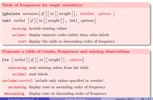
Discrete Variables

Table of frequences for single variable(s)

tabulate varnameif inweight, tabulate_options tab1 varlist if inweight, tab1_options

missing include missing values

nolabel display numeric codes rather than value labels

sort display the table in descending order of frequency

Generate a table of counts, frequences and missing observations fre varlistif inweight, options

nomissing omit missing values from the table

nolabel omit labels

include(numlist) include only values specified innumlist

ascending display rows in ascending order of frequency

descending display rows in discending order of frequency

tex export LaTeX-formatted table

(43)

Discrete Variables

Cross-tabulation of 2 variables

tabulate varname1 varname2 if inweight, options

chi2 report Pearson’sχ2

exact (#) report Fisher’s exact test

gamma report Goodman and Kruskal’s gamma

column report the relative frequency within its column of each cell

row report the relative frequency within its row of each cell

cell report the relative frequency of each cell

nofreq do not display frequencies (use only withcolumn,roworcell)

summarize(varname3) report summary statistics (mean, sd) forvarname3

Cross-tabulation of more than 2 variables, by values tab2 varlist if inweight, options

(44)

Tables of Statistics

table

table rowvar colvar supercolvar if in weight , options where inrowvar

colvar supercolvar we put categorical variables (up to 3).

by(superrowvarlist)variables to be treated as superrows (up to 4)

contents(clist)contents of the table’s cells, whereclistmay contain up to 5 statistics

mean varnamemean

sd varnamestandard deviation

sum varnamesum

n varnamecount of nonmissing observations

max,min varnamemaximum and minimum value

median varnamemedian

p1... p99 varnamepercentiles

iqr varnameinterquartile range (p75-p25)

(45)

Tables of Statistics

tabstat

tabstat varlist if in weight

, by(varname) options

where invarlistwe place a list of continuous variables, inby(varname)a categorical variable and among theoptionsinstatistics() we can choose:

mean n sum max,min sd

cv coefficient of variation (sd/mean)

semean standard error of mean (sd/sqrt(n))

skewness index of skewness

kurtosis index of kurtosis

p1... p99

range = max - min

(46)

Sample Tests

Tests apply to variables and allow to compare statistical significance of estimates against a null hp on the whole sample or for its subgroups. You can also use the command to perform tests under subgroups mean equality for the same variable, once a dicotomus variable identifying groups is selected (use missing values in this dummy varible to select only two subgroups which do not exhaust the sample dimensionn). You can use thetest_commandito obtain t-tests from inputted data (n, sd, means) that you like to compare. Other more specific tests can be

downloaded and installed. Here is a list of general features:

Test for means equality: help ttest

Performs t-test for1)one variable sample mean equality to a constant2)one variable two subsample means equality3)two variables means equality4)two variables two subsample means equality. You can specify distributions.

Test for standard deviations equality: help sdtest

Performs t-test for1)one variable sample sd equality to a constant2)one variable two subsample sd equality3)two variables sd equality4)two variables two subsample sd equality. You can specify distributions.

(47)

Graphs

help graph

This is the general command for all graphs. From here you can start searching the graphic style that you need, for univariate or multivariate representations, as well as statistical constructions. This is the broadest family of graphics.

help twoway

This command applies to bivariate graphics. The objective is to obtain a classical 2 coordinates graph, like scatter plots, connected points, confidence intervals,

regression fit, distributions... One graph may contain different series (ex: time against income and consumption) or different objects (ex: observed and predicted values). Oncetwowayis declared, you have to select (in pairs) the variables that you want to put in the same graph and thetypeof graph linking the two variables (ex:

scatter; connected; lfit; tsline; bar; spike; mband; lpoly;

function;...). In this way,graphs are built sequentiallyand all the objects will appear in the same space. You can add graphsoptions by looking at thehelp. Usingby(), you obtain separeted graphs according to the variable you want to be conditioned to. Optionsandin, ifmust be specified foreach graphic toolyou use, bacause they refer to a particular set of data in use.

(48)

Regression Analysis

Stata econometrics models can be included into 5 large families, but only the first one will be analysed. You are invited to read on thehelpthe full characterization of commands. In eachhelpfile you also find examples and interpretations of output results.

1) Cross-section econometrics

You are invited to look athelp regressfor the admissible regression commands, including OLS, IV, limited dependent variables methods, treatment effects models, censoring and selection bias corrections, 3SLS, systems of equations, quantile regression. Using the commandhelp regress_postestimationyou also obtain information on post-estimation tests and model application syntax.

2) Time series econometrics

You are invited to look athelp time, you will find all the list of commands associated with time series estimations, and how to build econometrics models in Stata. In particular,help tssetcan be used to declare a time series structure of your data, and than proceed with usual regression techniques. Using the command

help regress_postestimationtsyou also obtain information on post-estimation tests and model application syntax.

(49)

Regression Analysis

3) Panel data econometrics

You are invited to look at help xt, you will find all the list of commands associated with the panel dimesion of a database. In particular,help xtreg offers a wide explanation of panel-data analysis techniques, while with help xtreg_postestimationyou also obtain information on post-estimation tests and model application syntax.

4) Survey data analysis

Seehelp surveyfor all the details on data setting and regression techniques 5) Spatial econometrics

Seehelp spatregorspatwmatfor geographically located data. Commands available for Stata 10 or superior.

(50)

Regression Analysis

Common models: OLS, IV, probit, multiple logit

regress depvar indepvars if in weight , noc options ivregress estimator depvar varlist1 (varlist2=varlist_iv)

if inweight, noc options

probit depvar indepvars if inweight, options

mlogit depvar indepvars if inweight, options

options

refers to regression specific options or estimation

correction (robust se, constant...)

estimator

IV can be performed by 2SLS, GMM or limited info max

likelihood.

(51)

Regression Anlysis

Other regression models: List I

areg an easier way to fit regressions with many dummy variables

arch regression models with ARCH errors

arima ARIMA models

boxcox Box-Cox regression models

cnreg censored-normal regression

cnsreg constrained linear regression

eivreg errors-in-variables regression

frontier stochastic frontier models

heckman Heckman selection model

intreg interval regression

ivregress single-equation instrumental-variables regression

ivtobit tobit regression with endogenous variables

newey regression with Newey-West standard errors

qreg quantile (including median) regression

reg3 three-stage least-squares (3SLS) regression

rreg a type of robust regression

sureg seemingly unrelated regression

(52)

Regression Anlysis

Other regression models: List II

tobit tobit regression

treatreg treatment-effects model

truncreg truncated regression

xtabond Arellano-Bond linear dynamic panel-data estimation

xtdpd linear dynamic panel-data estimation

xtfrontier panel-data stochastic frontier model

xtgls panel-data GLS models

xthtaylor Hausman-Taylor estimator for error-components models

xtintreg panel-data interval regression models

xtivreg panel-data instrumental variables (2SLS) regression

xtpcse linear regression with panel-corrected standard errors

xtreg fixed- and random-effects linear models

xtregar fixed- and random-effects linear models with an AR(1) disturbance

xttobit panel-data tobit models

(53)

Post Estimation

Any Post Estimation command must be used immediately after a

regression model, and in any case it refers to last estimates stored in

Stata memory. You can save any model with a name and then proceed

in post estimations recalling the model name.

Predict

calculates predictions, residuals, influence statistics, and the

like after estimation

Predict regression output as new data

predict type newvar if in , statistic statistic

xb linear prediction; the default

residuals residuals

rstandard standardized residuals

rstudent studentized (jackknifed) residuals

stdp standard error of the linear prediction

(54)

Post Estimation

Test linear hypothesis on coefficients test coeflist

test exp=exp =...

Test on residuals: normality and zero-mean sktest varname

ttest varname == 0 scatter/mband

Test on residuals: heteroskedasticity by graph and tests rvplot

estat hettest estat imtest whitetst

(55)

Post Estimation

Test on variables: influential values

dfbeta

Logic of the

dfbeta

test:

1

Estimation with the complete sample

2

Estimation without the i-th observation

3

Comparison

Test on variables: collinearity

vif collin

(56)

Overview

Programming is an advanced topic. Some Stata users live productive lives without ever programming Stata. Chapter 18 in StataUsers Guideis an extremely useful reference for beginners in programming. Programs and do-files are related: a do-file is actually a collections of programs, which you can either recalled from the ado-file library (updated or increased depending on user needs) or created by the user. Once a program is specified, Stata gives you only the final output. Recall that do-files and programs both contains and share the same Stata commands.

Moreover, programs may call other programs or do-files, and do-files may call other do-files or programs. In general, programs are defined in do-files. The objective of programs is to simplify your life by nesting a specific set of operations in a unique command, which is initially defined in your do-files, and then can be repeatedly used in the rest of your session. A program is a sort of flexible do-file: variables names and options remains unspecified and it can be used in other circumstances. Programs may also be saved as Stata commands in ado-file format in a specific library and you are therefore free to call the program at occurrance as a Stata command.

In this section we will surveymacros, local and global, which allow to simplify the writeing. We will also describeloopsand then move toprogram arguments. Next section overviews the output programs and matrix programming.

(57)

Macros

Macros are the variables of Stata programs. A macro is simply a name associated with some text or a equence of arguments and can belocalorglobalin scope. We focus on local macros, which are private information of a single program, and no other program can make use of them (otherwise, they are global macros).

Macros: local and global local lcname

, =exp | :extended_fcn | [‘]"[string]"[’] global glname

, =exp | :extended_fcn | [‘]"[string]"[’] Use=expwhen the macro name refers to a result of an expression, stored in memory under the macro name. You can use it later in further calculations. When "=" is omitted, Stata stores in memory only theexp, which can me recalled in other mathematical expressions.

Use "[string]" when the macro name refers to a particular string. The string may contains a set of variables names, commands options, or other.

When you recall macro names in programs or commands, always use ‘’ indicators: ‘lcname’and‘glname’

(58)

Macros

Modify macros: show macro directory, drop and list macros,

program macros

macro dir/drop/list/shift mname

mname . . . | _all

(59)

Loop

Alooptakes a list and then executes a command or a set of commands for each elements of the list. The element currently being worked on is stored in a macro so you can refert to it in the commands. The list to be looped over can be a generic list of variable, values and levels. The list can be saved in macros as well.

foreach

: looping over a list of variables

foreach lname { in|of listtype } list {

commands referring to ‘lname’

}

You repeat the list of commands for all variables in a varlist, recalling each time the variable by its macroname ‘lname’

Obviously, you need to write the commands only once, using ‘lname’ in place of each variable name.

Withlnameyou create a fictious macro variable wich looped over thelistof variables.

There are different possible lists to be used: useinwhen the list is named,of

(60)

Loop

forvalues

: looping over a list of values

forvalues lname = range {

commands referring to ‘lname’

}

Commands are looped on some particular values, expecially usefull whenif, inis used as a conditioning statement.

Again, values must be recalled by ‘lname’.

Nested loops

foreach lname { in|of listtype } list { forvalues l2name = range {

for each ‘lname’ in sequence, commands refer to ‘l2name’

} }

(61)

Programming

Programming: basic elements for programming program define pgmname

, nclass | rclass | eclass | sclass

byable(recall, noheader | onecall) properties(namelist) sortpreserve plugin

version Stata_version

syntax varlist if in, DOF(integer 50) Beta(real 1.0)

The rest of the program must be coded in terms of ‘varlist’, ‘if ’, ‘in’, ‘dof ’, and ‘beta’

(62)

Programming

This is the standard syntax for a command. Inside the program

you must spacify the operations that Stata must run when the

name of the new command runs.

Assign a name to the program by

pgmname

, which is used

afterwards as a new command.

version

allows to optimize the program efficiency according to the

version of stata specified

syntax

must be used to specifues the syntax of the new

commands, for example the type and number of variables

admitted, their order in execution, if and in options.

After, write te list of commands, loops, macros that generate the

souce of your personal command created by the program.

Use

quietly

before commands to force Stata not to give the

output of the commands run inside the program. To decompose

the

varlist

in variables according to a specific order, see

help

tokenize

.

(63)

Output: Interpreting

Results from computations are showed in the Results Window and stored in memory by the .logfile. You can paste your output directly on your paper (or in other spreadsheet to rework them) by using the tables reported in the .log file. Stata offers other opportunites to list estimates and coefficients in a proper way (ex. with standard errors between brackets) whithout requiring additional changes in estimates values. In this Programming section we will see how output coefficients, vectors (ex. the regression parameters), matrices (ex. the variance-covariance matrix of regression coefficients) or scalars (ex. the mean of a variable, its standard deviation, or an R2 estimation) can be properly represented and used. By matrix algebra, we can perform advanced econometrics on data.

Remember that all the syntax previously presented appliesexclusivelyto data stored in memory. To apply this syntax to your output coefficients (for example compute the average of average values obtained by bootstrapping) you need to transform your results in data format (i.e. add columns).

(64)

Show Estimates

Your code must be operable even after that changes in your data occurs (by merge

orappend). Therefore, you need to perform your tests or report coefficients

independently from your output windows results (ex: t-test for means). Stata allows to save the estimates as scalars or vectors/matrices. The general procedure is the following:

1 Perform your statistical procedures or your estimations (likesummarizeor

regress);

2 _{Save your results and estimates in the memory by using}_r()_or_e() respectively. In this way you generate a new object;

3 _{Use your objects or display them in the output files.}

Alternatively, save regression results outreg varlist

using filename

, options text opt.: nol; title(); addn()

coefficients opt.:bdec(); coefstar

significance opt.:se | p | ci | beta; bracket; 3aster stat opt.: addstat(r2, N, F); xstats

other opt.:replace; append

(65)

Show Estimates

A program by Ben Jann, called

estout

, allows to organize post

estimation results, in particular for single regressions, system of

equations, maximum likelyhood estimation and marginal effects. The

extreme frexibility granted by this command allows you to reproduce

directly in Stata a final version of the table that you can copy and past

on your paper or report, with the calssical representation of regressors

by row, models by columns, coefficients over standard errors in

parenthesis, a separate line for additional statistics. You can also save

the result as L

A

TEXcode of the table (by choosing the

style

option).

estout

must be used after estimation. If you works with multiple

models, you can stored in memory each model estimates by using

estimates store

, and then recall them with

estout

.

Useful commands:

estpost

,

eststo

,

tabstat

,

esttab

,

est save

,

(66)

Show Estimates

See

help postest

for a general description of post estimations

commands.

help estimates

provides all the info to store, use and

report estimates. All commands work iff there is some result stored in

the memory.

Show estimates

After statistics

: see

help return

After regressions

: see

help ereturn

Scalar define, after summary statistics or table are reported

scalar define scalar_name = exp

scalar list scalar_list

scalar drop scalar_list

(67)

Show Estimates

After a regression command, use:

To store estimates in the memory (usename of your model) estimates store name , nocopy

estimates dir

scalar drop name_list

To report statistics and estimates tables from modelname estimates stats namelist , n(#)

estimates table namelist , options

stats(N r2 ll chi2 aic bic rank)reports statistics in the table;

keep(coeflist);drop(coeflist)to eliminate some coeff from the table;

b(%9.2f), se, t, pspecify the format of coeff reported and additioal stats;

To use results

(68)

Work with Data as Matrices

Data can be exported as a

matrix

n

×

k

(a vector is a single column

matrix), any statistics or estimation can be performed and result listed

in the matrix format. New data created (ex., predictions) can be

transformed in data from matrices.

If you operate with matrices, use algebra to compute statistics (ex.

¯

X

= (e

0

e)

−1

e

0

X

), any other command will not be working. If you

transform matrices in data (see the data editor), you can use previously

seen commands. Use

help matrix

for an exhaustive review of

commands to be used. To perform more complicated computation or

build your program, use the

Mata

environment which allows to use

Stata more interactively. See

help mata

for review of commands,

available in Stata 9 or superior.

The Mata environment is build-in in the Stata environment, that is it is

possible to call Mata when working with the Stata coding. This is done

by using functions such as:

mata:

text

.

(69)

Work with Data as Matrices

Set the size of a matrix

set matsize #

Data

→

Matrix; Matrix

→

Data; Input Matrix

mkmat varlistif in, matrix(matname) nomissing rownames(varname)

svmat matname , names( col | eqcol | matcol | string ) matrix input matname = (#[,#...][\#[,#...][\[...]]])

Operations with matrices

(70)

Mata language

In general, Mata environment is opened by setting: mata; and closed by settingend. All the code in the middle works exclusively for the Mata environment, but not for the Stata environment. Hence, Stata and Mata act as two separated softwares. Mata exploits a Matlab (C++) type of language.

Mata allows to import/export data from Stata usingst_matrixorst_data. The philosophy of Mata consists in taking "views" of the data stored in Stata format, use them in a form of an×k matrix, and perform the needed operations on these data. In the Mata environment, one can constructfunctionsthat recall a sequence of operations in Mata language. These functions are, in fact, programs.

Use Mata and notmatrixto work with data: Mata is designed to deal with huge dataset, matrix language is useful to deal with post-estimation results. The logic to construct a program is: (i) construct Mata functions with the needed arguments, saved after your program; (ii) construct the main program in Stata, when needed you should transform your data into Mata matrices/data views; (iii) recall Mata functions with simple code lines, thus not making it necessary to open/close the Mata environment within a Stata program (which would give an error).

For more hints on Mata, seehttp://www.ssc.wisc.edu/sscc/pubs/4-26.htmand

optimizefor the optimization tool.

(71)

Advanced material

Generate a unique file with panel structure from a series of separate waves, each divided into separate.csv files. A simple program allows to merge these data without even opening them.

Construct the maps of some data, provided these data can be linked with the relevant maps, and then geocoded.

Construct a program for a Gini-type multi-dimensional inequality indicator. This involves not only the construction of the program itself, but some Mata programming based on loops and combinatorics.

Advanced graphics to represent distributions functions, quantiles of these distributions, and estimates plus confidence intervals for estimators based on these quantiles.

Construct a program for testing ISD1 and dominance in gap curves under the assumption of independence. This step involves the use of Stata programming as well as Mata programming/optimization, along with the rearrangement of the result in easily interpretable tables.

Repec

updated).

Nicholas J. Cox,

Stephen Jenkins

Philippe Van Kerm.