Detecting Stress During Real-World Driving Tasks
Using
Physiological Sensors
Jennifer A. Healey and Rosalind W. Picard
Abstract
This paper presents methods for collecting and analyzing physiological data during real world driving tasks to determine a driver’s relative stress level. Electrocardiogram, electromyogram, skin conductance and respiration were recorded continuously while drivers followed a set route through open roads in the greater Boston area. Data from twenty-four drives of at least fifty minute duration were collected for analysis. The data were analysed in two ways. Analysis I used features from five minute intervals of data during the rest, highway and city driving conditions to distinguish three levels of driver stress with an accuracy of over 97% across multiple drivers and driving days. Analysis II compared continuous features, calculated at one second intervals throughout the entire drive, with a metric of observable stressors created by independent coders from video tapes. The results show that for most drivers studied, skin conductivity and heart rate metrics are most closely correlated with driver stress level. These findings indicate that physiological signals can provide a metric of driver stress in future cars capable of physiological monitoring. Such a metric could be used to help manage non-critical in-vehicle information systems and could also provide a continuous measure of how different road and traffic conditions affect drivers.
Keywords
driver, stress, traffic, automobile, physiology, sensor, signal, affect, recognition, classification, correlate, computer, skin conductance, electromyogram, electrocardiogram, respiration
J. A. Healey is with Hewlett-Packard Cambridge Research Laboratory E-mail: [email protected]. Rosalind W. Picard is with the MIT Media Laboratory, Cambridge MA, USA.
I. Introduction
The increasing use of on-board electronics and in-vehicle information systems has made the eval-uation of driver task demand an area of increasing importance to both government and industry[1] and understanding driver frustration has been listed by international research groups as one of the key areas for improving intelligent transportation systems[2]. Protocols to measure driver workload have been developed using eye glance and on-road metrics, but these have been criticized as too costly and difficult to obtain [3], and uniform heuristics such as the 15-Second Rule for Total Task Time, designed to provide an upper limit for the total time allowed for completing a navigation system task, do not provide flexibility to account for changes in the driver’s environment [3]. As an alternative, this study shows how physiological sensors can be used to obtain electronic signals that can be processed automatically by an on-board computer to give dynamic indications of a driver’s internal state under natural driving conditions. Such metrics have been proposed for fighter pilots[4] and have been used in simulations[5], but have not been tested on stress levels approximating a normal daily commute using sensors that do not obstruct drivers’ perception of the road.
This experiment was designed to monitor drivers’ physiologic reactions during real-world driving situations under normal conditions. Performing an experiment in real traffic situations ensures that the results will be more directly applicable to use in these situations; however it imposes constraints on the kinds of sensors that can be used and the degree to which experimental conditions can be controlled. Within these constraints, two types of analysis were performed on the collected signals. Analysis I was designed to recognize three general stress levels: low, medium, and high using five minute intervals of data from well defined segments of rest, city and highway driving. For this analysis, features from all sensors were combined using a pattern recognition technique and the different types of segments were recognized. Analysis II was designed to give a more detailed account of how individual physiological features vary with driver stress at each second of the drive, including those segments of the drive between the rest, city and highway segments. For this analysis a continuous metric of
observed stressors was created by scoring video tapes from individual drives. This metric was then correlated with features derived from each of the sensors on a continuous basis.
Historically, stress has been defined as a reaction from a calm state to an excited state for the purpose of preserving the integrity of the organism. For an organism as highly developed and independent of the natural environment as socialized man, most stressors are intellectual, emotional and perceptual[6]. Some researchers make a distinction between “eustress” and “distress,” where eustress is a good stress, such as joy, or a stress leading to an eventual state which is more beneficial to the organism[7], however in this paper we will refer to stress only as distress, stress with a negative bias, particularly distress caused by an increase in driver workload. There have been a number of studies that link highly aroused stress states with impaired decision making capabilities[8], decreased situational awareness[9] and degraded performance[10] which could impair driving ability.
This paper presents a method for measuring stress using physiological signals. Physiological signals are a useful metric for providing feedback about a driver’s state because they can be collected continu-ously and without interfering with the driver’s task performance. This information could then be used automatically by adaptive systems in various ways to help the driver better cope with stress. Some examples of this might include automatic management of non-critical in-vehicle information systems such as radios, cell phones and on-board navigation aids[2]. During high stress situations cell phone calls could be diverted to voice mail and navigation systems be programmed to present the driver with only the most critical information to help reduce driver workload. In addition, the music selection agent agent might lower the volume, or offer a greater selection of relaxing tunes to help the driver cope with their feelings of stress. Conversely, in low stress situations, the car might recognize that more driver distractions could be tolerated and provide the driver with more entertainment options.
The recognition algorithm presented in Analysis I could be run in real time by having the on-board computer keep a continuously updated record of the data from the last five minutes of the drive in memory and performing the analysis continuously on this window of data. Although none of the
physiological signals monitored here react quickly enough to contribute to automatic vehicle control, this kind of continuous monitoring, with a one to three minute lag in driver state assessment, is fast enough to initiate customized changes to the driver’s in-vehicle environment to help mitigate emotional distress. For example in high stress situations, some users might prefer visual navigation prompts to turn off or dim, since these types of warnings have been found to have a negative impact on situational awareness[9]. Alternatively, if intelligent collision avoidance were safely available in low velocity traffic jams, driving could become completely automated in such situations and a frustrated driver could relax by watching a movie or by working on their laptop.
A real time implementation would have been difficult to test on this driving route because the stress levels for the driving conditions outside of the rest, city and highway segments was not well defined by the design. To better assess the stress conditions of the entire drive, Analysis II looked at sixteen drives individually and created a continuous record of observable stressors from video tapes of the entire drive. This analysis also calculated continuous variables for each of the sensors and compared them to a continuous metric stress indicators scored throughout the entire drive. These variables were evaluated to determine which features provided the best single continuous indicator of driver stress. In new concept cars, such as the Toyota Pod car, continuous signals that correlate highly with stress level could be used to control the expressive changes in the cars lights and color[11], perhaps alerting others to the extra load on that driver. Furthermore, using aggregate continuous records of driver stress over a common commuting path, city planners could help quantify the emotional toll of traffic “trouble spots” which could help prioritize road improvements.
II. Driving Protocol
The driving protocol consisted of a set path through over 20 miles of open roads in the greater Boston area and a set of instructions for drivers to follow. Although stressful events could not be specifically controlled on the open road, the route was planned to take the driver through situations
where different levels of stress were likely to occur, specifically, the drive included periods of rest, highway and city driving that were assumed to produce low, medium and high levels of stress. These assumptions were validated by two methods: a driver questionnaire and a score derived from observable events and actions coded from video tape taken during the drives. The route was designed to reflect a typical daily commute so that the recorded stress reactions would all be within the range of normal daily stress.
To participate in the experiment, drivers were required to have a valid driver’s license and to consent to having video and the physiological signals recorded during the drive. Before beginning, drivers were shown a map of the driving route and given instructions designed to keep the drives consistent, for example, instructions were given to obey speed limits and not to listen to the radio. During the drive, an observer accompanied the driver in the car to answer any of the driver’s questions, to monitor physiological signal integrity and to mark driving events in the video record. The observer sat in the rear seat diagonally in back of the driver to avoid interfering with the drivers’ natural behavior.
All drives were conducted in mid-morning or mid-afternoon when there was only light traffic on the highway. Two fifteen-minute rest periods occurred at the beginning and end of the drive. During these periods the driver sat in the garage with eyes closed and with the car in idle. The rest periods were used to gather baseline measurements and to create a low stress situation. After the first rest period, drivers exited the garage through a narrow, winding ramp and drove through side streets until they reached a busy main street in the city. This main street was included to provide a high stress situation where the drivers encountered stop and go traffic and had to contend with unexpected hazards such as cyclists and jaywalking pedestrians. The route then led drivers away from the city, over a bridge and onto a highway. Between a toll at the on-ramp and a toll preceding the specified off-ramp, drivers experienced uninterrupted highway driving. This driving was included to create a medium stress condition. After the exit toll, drivers followed the off-ramp to a turn around and re-entered the highway heading in the opposite direction. After exiting the highway, the drivers returned through the city, down the same
busy main street and back to the starting point. The relative duration of these events can be seen in Figure 3. The total duration of the drive, including rest periods, varied from approximately fifty minutes to an hour and a half, depending on traffic conditions. Immediately after each drive, subjects were asked to fill out the subjective ratings questionnaires.
A. Data Collection
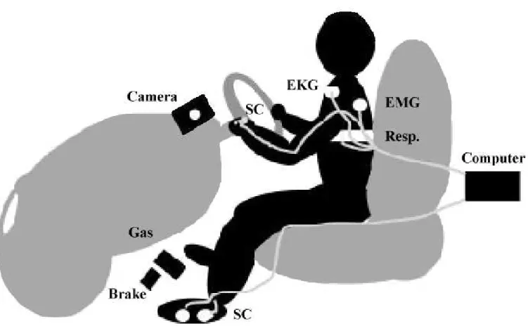
Four types of physiological sensors were used during the experiment: electrocardiogram (EKG), electromyogram (EMG), skin conductivity (also known as EDA, electro-dermal activation and GSR galvanic skin response) and respiration (through chest cavity expansion). These sensors were connected to a FlexComp[12] analog to digital converter which kept the subject optically isolated from the power supply. The FlexComp unit was connected to an embedded computer in a modified Volvo S70 series station wagon. The EKG electrodes were placed in a modified lead II configuration to minimize motion artifacts and maximize the amplitude of the R-waves since both the heart rate[13] and heart rate variability[14][15] algorithms used in this analysis depend on R-wave peak detection. The EMG was placed on the trapezius (shoulder), which has been used as an indicator of emotional stress[16]. The skin conductance was measured in two locations: on the palm of the left hand using electrodes placed on the first and middle finger and on the sole of the left foot using electrodes placed at each end of the arch of the foot. Respiration was measured through chest cavity expansion using an elastic Hall effect sensor strapped around the driver’s diaphragm. Figure 1 shows the general placement of sensors with respect to the automotive system.
The physiologic monitoring sensors were chosen based on measures previously recorded in real world driving and flight experiments. Helander (1978)[17] used an electrocardiogram (EKG), skin conduc-tivity and two EMG sensors to monitor drivers on rural roads. Heart rate and skin conductance have been used to monitor task demand on pilots [18] [19] [20] [21] as have EMG [20] and respiration[5] [20]. EMG [16] and skin conductivity [22] and heart rate variability[23] have also been studied as a general
indicators of stress.
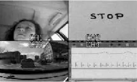
Each signal was sampled at a rate appropriate for capturing the information contained in the signal constrained by the sampling rates available on the FlexComp system. The EKG was sampled at 496 Hz, the skin conductivity and respiration sensor were sampled at 31 Hz and the EMG was sampled at 15.5 Hz after first passing through a 0.5 second averaging filter. The signals were collected by an embedded computer in a modified car. The experimenter visually monitored the physiological signals as they were collected using a laptop PC running a remote display program. The video output from this laptop, displaying the physiological signals was fed into a quad splitter to create a composite video record together with the video output from three digital cameras: a small Elmo camera mounted on the steering wheel, a Sony digital video camera with a wide angle (0.42) lens mounted on the dashboard and a third camera used for event. This record was used to create the continuous stress metric. A sample frame from one of the composite video records is shown in Figure 2.
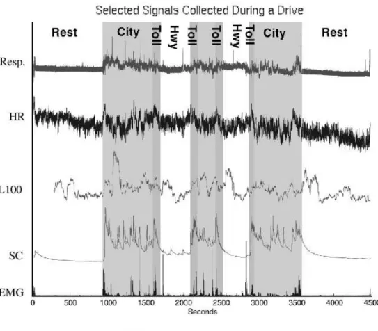
Figure 3 shows an example of the signals collected on a typical day’s drive along with markings showing driving periods and events. In total, 27 drives were completed, six by drivers who completed the course only once and seven each from three drivers who repeated the course on multiple days. In the first analysis, 24 complete data sets were used. Of the initial 27, one data set was incomplete because the hand skin conductivity sensor fell off, one data set could not be used because the EKG signal was too noisy to extract the R-R intervals necessary for the heart rate and heart rate variability metrics and one data set was lost because it was accidentally overwritten. In the second analysis all 16 drives were used for which video records were created (see Section V).
III. Questionnaire Analysis
The questionnaire analysis was used to validate a perception of low, medium and high stress during the rest, highway and city driving periods. Two kinds of ratings were used: a free scale and a forced ranking of events. The free scale section asked drivers to rate driving events on a scale of “1” to “5”
Condition Overall Comparative rating (1-5) rating (1-7) µ σ µ σ Rest 1.16 0.88 0.81 1.68 Highway 2.00 0.92 2.69 1.50 City 2.55 1.02 4.01 1.56 TABLE I
The Overall and Comparative questionnaire rating results after using a z-score and back transformation. The results of ANOVA analysis found the three states to be significantly
different at the 95% confidence level with p>0.001 for both the ratings
where a rating of “1” was used to represent a feeling of “no stress” and a “5” was used to represent a feeling of “high stress.” The forced scale section required drivers to rank events on a scale of 1 to 7 where “1” was assigned to the least stressful driving event and “7” to the most stressful driving event. Using this scale, drivers were asked to rate a number of events including encountering toll booths, merging and exiting as well as the rest, city and highway driving tasks. The extra categories were used to help drivers define the scale, but were not used in the questionnaire analysis.
For each questionnaire, the values for the both stress ratings were normalized using a z-score (z =
x−µ
σ )[24], then the average and standard deviation were calculated and back-transformed. The results,
see Table I, show that subjects found the rest periods to be the least stressful, the highway driving to be more stressful and the city driving to be the most stressful. ANOVA analysis on the z-score transformed variables determined that the means were significantly different at the 95% confidence level with p >0.001 for both the Overall and Comparative ratings. These results support the assumptions of the experimental design.
IV. Video Coding
The composite video record of the drives were coded to help assess driver stress levels. Two video coders scored each video tape record based on a list of observable actions and events that might correspond to an increase in driver stress. This list of potential stress indicators included including
stops, turning, bumps in the road, head turning and gaze changes. The coders were also allowed to use their judgment and score any number of additional events in an “other” column. The two coders analyzed the video tapes by advancing them at one second intervals and recording the number of stress indicators in each frame. For each drive, an average of over 25,000 frames were scored. Due to time limitations, this process was only completed for 16 of the 24 drives. The two coders were not involved in other aspects of the analysis. To test the inter-coder reliability Cronbach’s alpha[25] was calculated for a drive that was scored independently by both coders. These results were α = 1.0 for the highway segments, α =.91 for the city segments and α =.97 for the highway segments. Since all a coefficient of .80 is considered acceptable for most applications, these scores show that the rating system yielded consistent results between coders.
To create a stress metric, the number of stress indicators was first summed over each second of the drive. For example, if the driver was turning the steering wheel, changing gaze and turning his or her body during a frame, that frame would get a score of “3”. If the driver was driving straight and only looking around for a turn the frame would get a score of “1”. If no stress indicator was observed the score was entered as “0.” The sum of stress indicators at each second n of the drive was recorded in a time series Id(n) for each drive, d.
To further validate the assumption of low, medium and high stress conditions during the rest, highway and city segments, the time series Id(n), were averaged over each type of segment for all 16
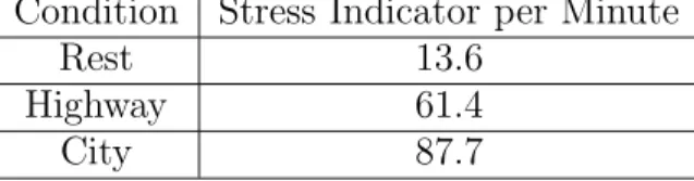
drives, d, and divided by the time of each segment time, T, to obtain an estimate of the number of stressors per minute for each type of driving. The results, shown in Table II, support the assumption of the design by showing that the greatest concentration of stress indicators occurred during the city driving condition, followed by fewer stress indicators during highway driving and the least during the rest conditions. As shown by the results, the rest conditions were not completely free of stress. During these periods some drivers would display restlessness by moving around, shifting position and reacting to noises from a nearby road. Some fidgeting may also have come from the initial discomfort of wearing
Condition Stress Indicator per Minute
Rest 13.6
Highway 61.4
City 87.7
TABLE II
The average number of stress indicators per minute during each of the three driving conditions: rest, highway and city
the sensors, boredom, or anticipation of either the beginning or end of the experiment. In one case the driver needed to use the rest room during the end rest period. The rest periods were not designed to keep the subject entirely free from stress, but to provide a lower stress situation just as city driving was designed to provide a higher stress situation.
V. Creating a Continuous Stress Metric
A continuous stress metric was created to develop a finer grain picture of the stressors encountered throughout the drives on various days. Although each drive contained thirty minutes of driving within the rest, city and highway conditions, it also contained approximately forty minutes of driving under other conditions that were not well defined by the experimental design. Unlike laboratory experiments where repeatable stress conditions can be created and controlled, the real world driving conditions encountered in this experiment were largely unpredictable and uncontrollable. The stress metric was designed to give a rough approximation of driver task load by counting the number of stress indicators at each second of the drive and smoothing the signal to incorporate the effect of anticipation and past events.
The video code scores captured a continuous record of all stress indicators that occurred throughout the drive, reflecting individual differences in driver reactions and varying traffic conditions. A con-tinuous stress metric was developed from these scores to be correlated with each of the time series of physiological features calculated for that drive. To create this metric each stressor was convolved with a simple model of its assumed stress effect. The stress effect was modeled as having both anticipatory
and persistence effects. In a model for pilot workload, Sheridan and Simpson identified several types of mental workload tasks that preceded each observed task: operating tasks, monitoring tasks, and planning tasks. They modeled the effect of each of these as a continuous workload function spanning a period of time between when the pilot anticipated the task and when the task was completed[26]. This model implies that before a stressor is observed there is an increase in driver stress due to an-ticipatory, monitoring and planning effects. In addition, the expected physiological effect of a stressor occurs slightly after the stimulus and may take several seconds or several minutes to recover depending on the type of stimulus event[27]. It is also known that physiological reactions add non-linearly and depend on habituation effects and components of the individual’s physiology[27].
To precisely model the effect of each observed stressor, the anticipatory components of mental workload and the expected persistence of the physiological effect would have to be individually modeled for each observation, taking into account all previous and concurrent events and a model of each driver’s physiology. Such a model would have been too complex for this analysis. Instead, each observed event was modeled by using a 100 second Hanning window, H, centered on the observation to approximate these effects.
The 100 second window was chosen for several reasons: it approximates the time needed for auto-nomic signals such as the skin conductivity to extinguish, it is the same window as the shortest window used for heart rate variability and it provides a level of smoothing that allows the essentially discrete stressor metric to approximate a continuous signal.
This window was convolved with the metric of events for each drive Id to create a signal Vd that
represented the modeled effect of the stressors as stated in Equation 1.
Vd(n) =Id(n)⊗H (1)
time series. The results are shown in Table IV and discussed in the section Analysis II. VI. Data Analysis
The collected data were subject to two types of analysis. Analysis I used five minute intervals of data from well defined segments of the drive where drivers experienced low, medium and high stress situations to train an automatic recognition algorithm. Analysis II investigated how continuous physiological features, calculated at one second intervals throughout the entire drive, correlated with a metric of driver stress derived from video tape records.
A. Analysis I: Recognizing General Stress Levels
The algorithm for general level stress recognition was developed using features derived from five minute non-overlapping segments of data taken from each of the rest, city and highway driving periods. Each of these segments was designed to represent a period of low, medium or high stress. To ensure consistency in the stress conditions, the data segments were taken from specific parts of the drive. The segments for the low stress condition were taken from the last five minutes of the rest periods, giving subjects enough time to relax from the previous task. The segments for the medium stress condition were taken from a stretch of uninterrupted highway driving between two toll booths, after the driver had completed a merge onto the highway and was safely in the right hand lane. The segments for the high stress condition were taken after the driver turned onto a busy main street in the city.
Nine statistical features were calculated for each segment: the normalized mean of the EMG and the normalized mean and variance for respiration, heart rate and skin conductivity on the hand and on the foot. The EMG, respiration and heart rate signals were normalized by subtracting the mean of the first rest period before each drive. The skin conductivity signals were normalized by subtracting the baseline minimum and dividing by the baseline range[16]. Heart rate was uniformly sampled and smoothed using a heart rate tachometer[13][28].
each of four bands. The power spectrum was calculated using 2048 data points from the middle of each segment. A Hanning window was applied and an implementation of Welch’s averaged, modified periodogram method[29] was used to calculated the normalized power spectrum. Four spectral power density features were calculated by summing the energy in the bands 0-0.1Hz, 0.1-0.2Hz, 0.2-0.3Hz and 0.3-0.4Hz. These features were found useful for discriminating emotion in previous work [30].
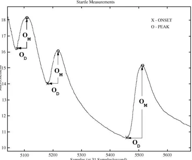
Eight additional skin conductivity features were calculated to characterize orienting responses. An orienting response is a sudden rise in the skin conductance due to ionic filling of the skin’s sweat glands in response to sympathetic nervous activation. A series of three orienting responses is shown in Figure 4, along with the marks indicating the onset and peak of the response and the measurements of the magnitude, OM, and duration, OD, of the response. The algorithm detected the onsets and peaks of
the orienting responses by first detecting slopes exceeding a critical threshold and then finding the local minimum preceding that point (onset) and the local maximum following that point (peak)[31]. Using this algorithm four orienting response features were calculated: the total number of such responses in the segment, the sum of the startle magnitudes ΣOM, the sum of the response durations ΣOD and a
sum of the estimated areas under the responses Σ(1
2OM∗OD). These four features were calculated for both the hand skin conductance and the foot skin conductance signals.
The final feature was a heart rate variability (HRV) feature which has been used to representing sympathetic tone. The parasympathetic nervous system is able to modulate heart rate effectively at all frequencies between 0 and 0.5 Hz, whereas the sympathetic system modulates heart rate with significant gain only below 0.1Hz[32]. By taking the ratio of the low frequency heart rate spectral energy to the high frequency heart rate spectral energy we derive a feature that represents the ratio of the sympathetic to parasympathetic influence on the heart. Our hypothesis is that increased stress will lead to an increase in sympathetic nervous activity and an increase in this ratio.
To calculate the HRV feature, we used the instantaneous heart rate time series derived from the EKG. A Lomb periodogram[15] was used to calculate the power spectrum[33][34] of the heart rate time
series because it can directly use unevenly sampled inter-beat interval data and because it is robust to missed beats[35]. The total energy in the low frequency (LF) band (0-0.08 Hz) and in the high frequency (HF) band (0.15Hz-0.5Hz) were calculated and the ratio LF
HF was used as the final feature.
In Analysis II, another suggested sympatho-vagal balance ratio, LF+M F
HF , using the mid-frequency (MF)
range (0.08Hz-0.15Hz) was also used along with a shorter window size.
These 22 features were used to create a single vector representing each of the segments used in the recognition analysis. A total of 112 segments were used: 36 from rest periods, 38 from highway driving and 38 from city driving. The resulting 112 feature vectors were then used to train and test the recognition algorithm. Each vector was sequentially excluded from the training set and the recognition algorithm was trained using the remaining 111 vectors. The training vectors were used to create a Fisher projection matrix and a linear discriminant. The Fisher projection was determined by solving a factorization for the generalized eigenvectors of the covariance matrices for the between class scatter and the within class scatter of the labeled training vectors[36]. The generalized eigenvectors corresponding to the two greatest eigenvalues were used to project the 22 dimensional feature vectors onto a two dimensional space where the between class scatter was maximized and the within class scatter was minimized. Using the projection determined by the training data the test vector y was projected into a two dimensional vectorˆy. In the two dimensional space, a linear discriminant function
gc(ˆy) was determined using the sample mean (mc) and the a priori probability P r[wc] for each class
c and pooled covariance K of the training vectors. The test vector was classified as belonging to the class for which gc(ˆy) was the greatest.
gc(yˆ) = 2m T cK −1 ˆ y−mTcK −1 mc+ 2ln(P r[wc]); (2)
Table III is a confusion matrix for the recognition algorithm in which all correctly classified segments are shown along the diagonal and all incorrectly classified segments are off diagonal. As this table
Recognition Results Labeled As
Recognized as: Low Medium High Recognition Rate
Low 36 0 0 100%
Medium 0 36 1 94.7%
High 0 2 37 97.4%
TABLE III
The confusion matrix for the recognition algorithm. Correctly recognized segments are found along the diagonal. This classifier mistakenly classified two medium stress segments as high stress
and one high stress segment as medium stress.
shows, all low stress segments were correctly recognized but two periods that were labeled as medium stress were recognized as being high stress and one period labeled as high stress was classified as medium stress. The results thus show very good discrimination between the classes. These physiologically based results also show a perfect discrimination between the low stress rest period and the two driving periods which agrees with both the perception of stress as evaluated by the questionnaire and the scoring of observed stressors obtained from the video tape analysis, suggesting that these features accurately represent a driver’s general stress level.
B. Analysis II: Continuous Correlations
The recognition algorithm gives good separation between three general types of driving stress, but it does not account for variations in the drives and it does not give a fine grain assessment of stressors. An ideal indicator of stress would be a physiological variable that continuously varied proportional to every driver’s internal stress. To determine which features might be the best candidates for such a variable, continuous calculations were made on each of the physiological sensor signals at one second intervals throughout the entire drive for each of the sixteen drives for which the video was scored. These calculations included the mean and variance of the EMG (µE, σ2E), hand skin conductivity (µS,
σ2
S), respiration (µR, σR2) and the mean of the tachometer heart rate (µH) over one second intervals
For this analysis four metrics of heart rate variability were calculated. In addition to the 300 second window LF
HF used in Analysis I, a 100 second window and a
LF+M F
HF were also calculated for comparison.
These time series are denoted: L100, M100, L300 and M300 for the LF
HF (L) and
LF+M F
HF (M) power
ratios in the 100 and 300 second periodograms respectively. To create a continuous time series, Lomb periodograms were calculated using both 100 and 300 second windows (Hanning) of instantaneous heart rate data, centered on the second of interest, advanced by one second for each second of the drive. The 150 seconds at the beginning and end of the drive were excluded because there would not have been enough data for the periodogram.
For each of the drives d, the video stress metricVd(n) was correlated with each of the feature time
series and a correlation coefficient rd was calculated:
rd =
KV P
σV V ∗σP P
(3)
where KV P is the covariance of the time series Vd(n) with one of the physiological time series for the
same drive d and σV V and σP P are the standard deviations for Vd(n) and physiological time series,
respectively.
If the feature time series were independent of the stress metric, the correlation coefficient would be zero. To test this null hypothesis, each of the stress metrics was also correlated with a white noise signal w. Table IV shows the results for each time series for all sixteen drives. As expected, the correlation coefficients with white noise, w, were all close to zero. The variance of the EMG, σ2
E, and the mean of the respiration,µR, were also close to zero. This was also expected, since the EMG signal was pre-processed with a smoothing filter and the respiration mean primarily represents the baseline stretch of the sensor which varies mostly with sensor movement (slippage) with respect to the chest cavity. The variance of the respiration, σ2
R, and the variance of the skin conductivity, σ2
G, also did not correlate well with the stress metric, most likely because the variance over one second intervals in
Day L100 L300 M100 M300 HR µE σE2 µG σ2G µR σR2 w S1-2 .53 .61 .53 .64 .34 .22 .01 .75 .09 -.53 .04 .01 S1-3 .45 .45 .44 .42 .35 .04 .01 .77 .08 -.49 .04 .00 S1-4 .45 .58 .47 .60 .53 .14 .06 .71 .18 -.33 .26 .01 S1-5 .41 .35 .22 .09 .46 .30 .08 .85 .22 -.22 .15 .01 S1-6 .62 .62 .59 .62 .31 .32 .09 .74 .00 -.56 .16 .01 S1-7 .46 .36 .41 .31 .52 .28 .04 .77 .23 -.23 .16 .01 S2-2 .49 .66 .55 .69 .49 .02 .03 .13 .00 -.24 .15 -.01 S2-4 .22 .29 .13 .17 .41 .27 .01 .59 .12 .12 .18 .00 S3-2 .74 .73 .75 .74 .44 .20 .06 .78 .20 .17 .25 -.01 S3-4 .46 .41 .48 .48 .38 .16 .06 .77 .15 .59 .19 .01 S3-5 .41 .51 .44 .50 .35 .09 .00 .81 .20 .21 .01 -.02 S3-6 .44 .53 .44 .51 .40 .20 .04 .73 .14 .67 .24 .03 S3-7 .35 .35 .39 .35 .29 .22 .08 .78 .16 .44 .12 -.01 R2-1 .41 .58 .39 .54 .30 .20 .06 .47 .06 .10 .03 .00 R3-1 .32 .42 .35 .41 .30 .16 .13 .45 .08 .03 .10 .01 R4-1 .49 .55 -.08 -.19 .76 .37 .09 -.07 .03 -.28 .22 -.03 µ-zs .52 .60 .49 .57 .48 .17 .03 .99 .08 -.42 .10 -.01 µ-zt .50 .56 .45 .49 .45 .20 .05 .81 .12 -.03 .15 .00 TABLE IV
Correlation coefficients “rd” between the stress metric created from the video and variables
from the sensors indicating how closely the sensor feature varies with the stress metric. As a null hypothesis, a set of random numbers, “w” was also correlated with the video metric for each
drive. The last rows show the mean over all days as calculated by using the z-score and z-transform methods respectively.
these signals has a large noise component.
To determine which sensors might be most useful for use as a real time indicator of stress, the averages of the correlation coefficients were calculated in two ways, first by calculating a z-score for each day’s scores, averaging and then back transforming to get the result shown in row “µ-zs” and second by using the normalizing z-transform, zd = 0.5∗(ln(1 +rd)−ln(1−rd)), and averaging to
get the result shown in row “µ-zt.” The z-score transformed data is more likely to be robust against a poor stress metric on a given drive and the z-transformed data creates a more normal distribution of the data, which may give a better estimate of the true mean. Both transformations yield similar results suggesting that skin conductivity is the best real-time correlate of stress followed by the heart rate variability and heart rate measures. In general, the skin conductance performed well (with the
notable exceptions of drives S2-2 and R4-1) and the heart rate variability measures performed similarly to each other, with the exception of drive R4-1, where the two metrics using LF+M F
HF ratio correlated
differently than the two metrics using the LF
HF ratio. The 100 second and 300 second windows for
HRV performed similarly, suggesting that it is possible to use the shorter 100 second window to derive features for HRV, although this window excludes some of the low frequency power typically used in HRV calculations. The mean heart rate,µR, was the best correlated measure for only one of the drives. There were individual differences in how drivers responded. In Drive S3-2, there were very high correlations for both the mean skin conductivity and for the average HRV measures, however Drive S2-4 showed a much stronger correlation with skin conductivity and heart rate than with HRV measures and Drive S2-2 showed a weak correlation with skin conductance and stronger correlations heart rate and HRV measures. For all drivers studied, the lowest correlation between either the heart rate or skin conductance metrics was 0.49, suggesting that between these two sensors a reliable metric can be obtained. These correlations were performed over approximately 25,000 sample points per drive. It is not clear from these results if individuals consistently respond to stress with similar physiological reactions. For S1 and S3 there was less variance in mean skin conductance response for the same subject over many drives than for all subjects over all drives and for S1 the same was also true of heart rate variability. We performed ANOVA anaylsis on the correlation coefficients and found significant individual differences in the mean of the skin conductance µG (p = 0.0007) and the mean of the respiration µR (p = 0.0001). The difference in the mean skin conductance is most observable for subject S3. This may be due to a physiological difference in the number of sweat glands on the palm or from a different in electrode contact due to the way the subject gripped the steering wheel. The differences in the respiration means are most likely due to physical differences in chest size.
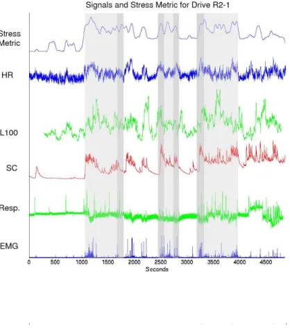
Figure 5 shows an example of the stress metric plotted against signals from drive R2-1. For this drive, the best correlating signal shown is the mean of the skin conductivity (.47) followed by L100 (.41) and heart rate (.30). This graph shows qualitatively how well each of the signals reflects the
stress metric. During this drive, the subject was unusually agitated during the second rest period due to a need to use the restroom. This agitation is reflected in the stress metric, but would not have been taken into account by using the task based categorization.
VII. Discussion
In the future, we may want vehicles to be more intelligent and responsive, managing information delivery in the context of the driver’s situation. Physiological sensing is one method of accomplishing this goal. This study tested the applicability of physiological sensing for determining a driver’s overall stress level in a real environment using a set of sensors that do not interfere with the driver’s perception of the road. The results showed that three stress levels could be recognized with an overall accuracy of 97.4% using five minute intervals of data and that heart rate and skin conductivity metrics provided the highest overall correlations with continuous driver stress levels.
Using a continuously updated record of the last five minutes of a driver’s physiology, the stress recognition algorithm might be used to manage real-time, non-critical applications such as music selection and distraction management (cell phones and navigation aids, etc.), which could tolerate a delay in updating the user’s state precisely. The original five minute time window was chosen because it was the interval recommended for calculating heart rate variability using the spectrograms[23] and because the limiting time factor for the driving segments, the uninterrupted highway segment between the two toll booths, was just over five minutes long. In a similar study, Wilson et al. [5] trained an artificial neural network to recognize three levels of pilot task demand using five minute intervals of rest and low and high levels of difficulty on the NASA Multiple Attribute Task Battery during a simulation. For this experiment, heart rate, EEG, electrooculographic (EOG) and respiration data were used. The algorithm was first tested on the five minute training segments, then it was run continuously to detect stress in real time. When a high stress level was detected, the simulation adapted by turning off two of the subtasks, enabling a 33% reduction in errors. A similar test could be performed with the algorithm
developed in Analysis I if road conditions could be made constant and drivers could be allowed to make safe errors while talking on the cell phone or using visual navigation aids. If a high stress condition were detected using the algorithm on the last five minutes of data, the driver distractions could be turned off until the driver recovered to a medium stress level. The level of driver error for drivers using this adaptive aid could then be compared to a set of control drivers who did not have this feedback.
Although the original experiment was not designed to test how the five minute algorithm would perform in a real time scenario, the second analysis compared near real-time features to a continuous stress metric to determine how well these signals reflected driver stress on a continuous basis. Driver’s reaction time to specific stressors was not measured because the latencies involved fall beneath the resolution of the coding metric. For example, the skin conductivity latency is on the order of 1.4 seconds [37] and anticipatory EMG has been measured in the laboratory at 30 milliseconds[38]. In this experiment, the video was scored at one second intervals and the video clock and sensor clock were not synchronized to be sensitive to time differences within a few seconds. The latency measurements would also be confounded by the open road conditions where many stressors occurred concurrently and before the effects of previous stressors had extinguished.
Despite these limitations, these experiments show that physiological signals provide a viable method of measuring a driver’s stress level. Although physiological sensing systems have not yet developed to the point where they are as inexpensive and convenient to use as on board cameras, sensors are becoming smaller and researchers are developing new ways to integrate them into existing devices. The results of the second analysis suggest that the first sensors that should be integrated into a car, or a mobile wearable device that communicates with a car, should be skin conductance and heart rate sensors. These measures could be used in future intelligent transportation systems to improve safety and to manage in-vehicle information systems cooperatively with the driver.
Additionally, future computer vision algorithms and car sensors might be able to automatically calculate a stress metric similar to the one created by video coding analysis. Such methods might
provide an automatic non-contact method for predicting or otherwise anticipating changing levels of driver stress related to cognitive or emotional load.
Acknowledgments
The authors would like to acknowledge the comments of Dr. Roger Mark, Dr. Ary Goldberger, Joe Mietus, George Moody, Isaac Henry, Dr. Paul Viola, Dr. John Hansman. We would also like to thank George Moody for his EKG software and advice and our students Kelly Koskelin, Justin Seger and Susan Mosher for their assistance with the experiment. We would like to thank Media Lab’s Things That Think and Digital Life Consortia for sponsoring this research.
References
[1] Y. I. Noy. (2001) International harmonized research activities report of working group on intelligent transportation systems (ITS). Proceedings of the 17th International Technical Conference on the Enhanced Safety of Vehicles. [Online]. Available: http://www-nrd.nhtsa.dot.gov/pdf/nrd-01/esv/esv17/proceed/00134.pdf
[2] P. Burns and T. C. Lansdown. (2000) E-distraction: The challenges for safe and usable internet services in vehicles. NHTSA Driver Distraction Internet Forum. [Online]. Available: http://www-nrd.nhtsa.dot.gov/departments/nrd-13/driver-distraction/Papers.htm
[3] National Highway Traffic Safety Administration (NHTSA). Proposed driver workload metrics and methods project. [Online]. Available: http://www-nrd.nhtsa.dot.gov/departments/nrd-13/driver-distraction/PDF/32.PDF
[4] M. J. Skinner and P. A. Simpson, “Workload issues in military tactical aircraft,”Int. J. of Aviat. Psych., vol. 12, no. 1, pp. 79–93, 2002.
[5] G. F. Wilson, J. D. Lambert, and C. A. Russell, “Performance enhancement with real-time physiologically controlled adaptive aiding,”Proceedings of the Human Factors and Ergonomics Society 46th Annual Meeting, vol. 3, pp. 61–64, 1999.
[6] H. Selye,Selye’s Guide to Stress Research. Van Nostrand Reinhold Company, 1980.
[7] I. J. K. G. Eisenhofer and D. Goldstien, “Sympathoadrenal medullary system and stress,” in Mechanisms of Physical and Emotional Stress. Plenum Press, 1988.
[8] A. Baddeley, “Selective attention and performance in dangerous environments,”British Journal of Psychology, vol. 63, pp. 537–546, 1972.
[9] M. Vidulich, M. Stratton, and G. Wilson, “Performance-based and physiological measures of situational awareness,”Aviation, Space and Environmental Medicine, pp. 7–12, May 1994.
[10] R. Helmreich, T. Chidster, H. Foushee, S. Gregorich, and J. Wilhelm, “How effective is cockpit resource management training? issues in evaluating the impact of programs to enhance crew coordination,”Flight Safety Digest, vol. 9, no. 5, pp. 1–17, 1990.
[11] S. Newbury,The Car Design Yearbook. Merrell Publishers, 2002.
[12] ProComp Software Version 1.41 User’s Manual, Thought Technology Ltd., 2180 Belgrave Ave. Montreal Quebec Canada H4A 2L8, 1994.
[13] G. Moody. tach [c-language software]. [Online]. Available: http://www.physionet.org/physiotools/wag/tach-1.htm [1985] [14] ——. ihr [c-language software]. [Online]. Available: http://www.physionet.org/physiotools/wag/ihr-1.htm [2002]
[15] N. R. Lomb, “Least-squares frequency analysis of unequally spaced data,” Astrophysics and Space Science, vol. 39, pp. 447–462, 1976.
[16] J. T. Cacioppo and L. G. Tassinary, “Inferring psychological significance from physiological signals,”American Psychologist, vol. 45, no. 1, pp. 16–28, Jan. 1990.
[17] M. Helander, “Applicability of drivers’ electrodermal response to the design of the traffic environment,”Journal of Applied Psychology, vol. 63, no. 4, pp. 481–488, 1978.
[18] T. C. Hankins and G. F. Wilson, “A comparison of heart rate, eye activity, eeg and subjective measures of pilot mental workload during flight,”Aviation, Space and Environmental Medicine, vol. 69, pp. 360–367, 1998.
[19] J. A. Veltman and A. W. K. Gaillard, “Physiological indicies of workload in a simulated flight task,”Biological Psychology, vol. 42, pp. 323–342, 1996.
[20] G. F. Wilson, “An analysis of mental workload in pilots during flight using multiple psychophysiologic measures,” The International Journal of Aviation Psychology, vol. 12, no. 1, pp. 3–18, 2001.
[21] M. A. Bonner and G. F. Wilson, “Heart rate measures of flight test and evaluation,” The International Journal of Aviation Psychology, vol. 12, no. 1, pp. 63–77, 2001.
[22] W. Boucsein,Electrodermal Activity. New York, NY: Plenum Press, 1992.
[23] C. M. A. vanRavenswaaij et al., “Heart rate variability,”Annals of Internal Medicine, vol. 118, pp. 436–447, 1993. [24] E. Crow, F. A. Davis, and M. W. Maxfield,Statistics Manual. Toronto, Canada: General Publishing Company, 2002. [25] G. G. Berntson and J. T. B. J. et al., “Coefficient alpha and the internal structure of tests.” Psychometrika, vol. 16, pp.
297–333, 1951.
[26] T. B. Sheridan and R. W. Simpson, “Toward the definition and measurement of the mental workload of transport pilots,” Flight Transportation Laboratory, MIT Department of Aeronautics and Astronautics, FLT Report R79-4, Jan. 1979. [27] R. A. Sternbach,Principles of Psychophysiology. Academic Press, 1966.
[28] G. B. Moody and R. G. Mark, “Development and evaluation of a 2-lead ecg analysis program,” Computers in Cardiology, vol. 9, pp. 39–44, 1982.
[29] Matlab Version 5.3.0.10183 (R11) On-line User’s Manual, The Mathworks, Inc., 3 Apple Hill Drive,Natick, MA 01760-2098, 1999.
[30] R. Picard, E. Vyzas, and J. Healey, “Toward machine emotional intelligence,” IEEE Transactions on Pattern Analysis and Machine Intelligence, vol. 23, no. 10, pp. 1175–1191, 2001.
[32] G. G. Berntson and J. T. B. J. et al., “Heart rate variability: Origins, methods and interpretive caveats,”Psychophysiology, vol. 34, pp. 623–647, 1997.
[33] G. Moody. lomb [c-language software]. [Online]. Available: http://www.physionet.org/physiotools/wag/lomb-1.htm [1992]. [34] G. B. Moody, “Spectral analysis of heart rate without resampling,” Computers in Cardiology, vol. 20, pp. 715–718, 1993. [35] P. Laguna, G. B. Moody, and R. G. Mark, “Power spectral density of unevenly sampled data by least-square analysis:
performance and application to heart rate signals,”IEEE Trans Biomed Eng, vol. 45, pp. 698–715, 1998. [36] R. Duda and P. Hart,Pattern Classification and Scene Analysis. John Wiley & Sons, 1973.
[37] R. Lockhart, “Interrelations between amplitude, latency, rise time and the edelberg recovery measure of the galvanic skin response,”Psychophysiology, vol. 9, no. 4, pp. 437–442, 1967.
[38] Y. Barnif. (2001) Using electromyography to predict head motion for virtual reality. Research Report, NASA Ames Research Center, Human Factors Research and Technology Division, Human Information Processing Branch. [Online]. Available: http://human-factors.arc.nasa.gov/ihh/web/library/rt reports.php
Fig. 1. The subject wore five physiological sensors, an electrocardiogram (EKG) on the chest, an electromyogram (EMG) on the left shoulder, a chest cavity expansion respiration sensor (Resp.) around the diaphragm and two skin conductivity sensors (SC), one on he left hand and one on the left foot. The sensors were attached to a computer in the rear of the vehicle.
Fig. 2. A sample frame from the quad split video collected during the experiment. The upper left panel shows the driver facial expression, collected from a camera mounted on the steering column. The upper right panel shows the camera used for experimenter annotations where a “stop” annotation is shown. The lower left panel shows road conditions and the lower right panel shows a visual trace of the physiological signals as they were being recorded.
Fig. 3. This figure shows an illustration of the physiological data collected from the respiration, heart rate, L100 spectral ratio, the skin conductivity (SC) from the hand and the electromyogram (EMG). This figure does not show vertical units because each signal is scaled and offset to be shown with an illustrative amount of detail.
Fig. 4. An example of three orienting responses occurring in a one minute segment of the skin conductance signal. The onset as marked by the detection algorithm is marked with an “x” and peak is marked with an “o”. The magnitude
Fig. 5. This figure shows an illustration of the physiological data collected from the respiration, heart rate, L100 spectral ratio, the skin conductivity (SC) from the hand and the electromyogram (EMG) along with the stress metric derived from the video tapes for this drive. This figure does not show vertical units because each signal is scaled and offset to be shown with an illustrative amount of detail.