Improved Method for Predicting Software Effort and
Schedule
Wilson Rosa
IT Estimating Division Naval Center for Cost AnalysisCheryl Jones and John McGarry
US Army RDECOM-ARDEC [email protected]Ray Madachy
Department of Systems Engineering Naval Postgraduate School
Joe Dean
Air Force Cost Analysis Agency [email protected]
Barry Boehm and Brad Clark
Center for Systems and Software University of Southern California[email protected] [email protected]
ABSTRACT
This paper presents a set of effort and schedule estimating relationships for predicting software development projects using empirical data from 317 very recent US DoD programs. The first set predicts effort as a function of product size and application type. The second predicts the duration of software development as a function of product size and staffing levels. The estimating relationships are simpler and more viable to use for early estimates than traditional parametric cost models. Practical productivity benchmarks are also provided to guide cost analysts in normalizing and validating data. These methods are applicable to all industry sectors.
General Terms
Management, Measurement, Design, Economics
Keywords
COCOMO, software cost estimation, application domain, SEER-SEM, operating environment, application type
1.
INTRODUCTION
1.1
Problem Statement
Studies on software estimation tend to approach the analysis framework in any of three ways. A group of studies [1, 2, 3, 4, 5, 9] have assessed the COCOMO framework to help identify the main cost drivers. A second set of studies [10, 13, 14, 21] have examined the impact of fewer product attributes --application domain, personnel capability, reliability, defects -- on software productivity using local data. The evidence is almost uniform in indicating that application domain is the second major cost driver after product size.
Only a relative handful of studies [15, 16, 17, 20] have specially examined whether application domain stratification has a significant impact on software productivity. However, these studies are based on projects collected in the late 1990s and do not provide the data. Whether the degree of stratification has a direct impact on software cost remains an open question.
1.2
Purpose of the Study
This study attempted to contribute to the knowledge base by exploring the influence of grouping 34 application domains into 12 general complexity zones called Application Types. This study examines the direct effect of Application Types on software cost and schedule. It also provides the statistics and regression models upon which detailed estimates are based.
1.3
Paper Organization
This research paper is organized into nine sections:
Section 1 introduces deficiencies in past studies and proposed solution.
Section 2 summarizes the scholarly literature of related studies. In particular, it highlights previous domain-driven analyses and data grouping taxonomy.
Section 3 goes over the research method step by step. It briefly explains the survey method, instrumentation, data normalization framework, and criteria for selecting the best fit models.
Section 4 describes the data demographics, including segmentation, age of data, size, effort distribution percentages, and productivity benchmarks. Section 5 discusses the data analysis results. Section 6 presents the effort estimating models. Section 7 presents the schedule estimating models. Section 8 provides the research conclusions on the basis
of the hypotheses. It also highlights the contributions and limitations, and outlines areas for further research. Section 9 cites the sources used in the paper.
2.
RELATED WORK
Tan [20] pioneered a domain-based effort distribution model. The
goal of his dissertation work was to test the use of domain information to enhance the current COCOMO II effort distribution guideline to provide more accurate resource allocation
for software projects. Over 200 software projects from the U.S. Department of Defense data repository [19] were analyzed. The results support the use of application types on effort distribution estimation by rejecting the null hypothesis that the distributions do not vary by domains. The dissertation’s research method is very similar to this study in three ways. It used the same instrument, same data source, and similar application taxonomy.
Putnam and Myers [14] performed an empirical study to
determine the major contributors to software productivity variance. Sixteen hundred projects from the Quantitative Software Management Inc. (QSM) database were used in the study. To reduce variation and ensure valid comparisons, project data in the QSM database was stratified into 10 software application categories: Application Category Productivity Ranking (Lowest to Highest) Microcode 1 Firmware 2 Real-Time Embedded, Avionics 3 Radar Systems 4 Command and control 5 Process Control 6 Telecommunications 7 System Software 8 Scientific Systems 9 Business Systems 10
Results showed that after SIZE, the second most influencing factor on productivity was application category. The application categories and productivity ranking order (from lowest to highest) aligns with this study. Unfortunately the descriptive statistics and dataset are proprietary.
Jones, McGarry, Dean, Rosa, Madachy, Boehm, Clark, and Tan [12] introduced the concept of domain-driven software cost
estimation by grouping similar application domains together called Productivity Types. The purpose of this study was to present a set of open source effort and schedule estimation models by productivity types. The statistical models were based on empirical data collected from 250+ programs implemented within the US DoD. Results show that effort estimation models should account for the effect of fixed start-up costs and that the prediction accuracy is enhanced when dataset is grouped by productivity types. The productivity type definitions are the same used in this study but most of the data points are from projects implemented in the late 1990s.
Rosa, Boehm, Clark, Madachy, and Dean [17] continued their
investigation into domain-driven software estimation by updating their regression models using a more recent dataset (2004-2011) from 204 projects. It also introduced a set of software schedule estimation models based on product size and staffing levels. The authors reinforced their previous study by concluding that domain-driven analysis seems to be the best framework for simple effort estimation. Further, the study also concluded that size and staffing levels are valid predictors of software development
duration, as the prediction accuracy, PRED (30), on all cases was higher than 58%.
Rosa [18] introduced a schedule estimation model for Enterprise
Resource Planning projects. The model predicts the duration of software development phase as a function of SIZE and full time equivalent staff. The statistical analysis is based on empirical data collected from 22 programs implemented within the federal government over the course of ten years beginning in 2001. Result shows that software schedule estimation models should include both, product size and staffing levels as independent variables.
3.
RESEARCH METHOD
3.1
Research Question
This study will address the following questions:
Is Application Type a good predictor of software engineering labor, when treated along with size?
Does software development duration relate to size and staffing levels, when grouped by Application Type?
3.2
Quantitative Method
A survey method was used in this study to collect effort and cost drivers of software development projects. A non-random sample was used since the researcher had access to names in the population and the selection process for participants was based on their availability.
3.3
Population and Sample
The sample was identified as 317 software projects that have been implemented for the United States Department of Defense (DoD). These projects were completed during the time period from 2004 to 2012. The number of projects considered for effort analysis was 317. However, the number of observations available for schedule analysis (213 of 317) was lower, as some projects had incomplete schedule data.
3.4
Instrumentation
Data were collected by means of a questionnaire containing over 20 items. The data collection questionnaire used in the study was obtained from an existing one; Software Resource Data Report
(SRDR) questionnaire [19]. The source questionnaire entitled
“SRDR Sample Formats” can be downloaded from the Defense Cost Analysis Resource Center (DCARC) website:
http://dcarc.cape.osd.mil/Files/Policy/2011-SRDRFinal.pdf http://dcarc.cape.osd.mil/Files/Policy/Final_Developer_Report.xlsx The questionnaire collected data on product size, effort, schedule and product attributes like required reliability, software process maturity, etc. A new field was added to collect data on application domain. The list of application domains and definitions are from available instrument [6].
3.5
Data Normalization
The objective of data normalization is to improve data consistency, so that comparisons and projections are more valid.
The software data set in this study was normalized using three steps:
3.5.1
Converting to Equivalent Size Unit
Since the dataset captures project size by type (new, modified, reused, auto generated) and adaptation adjustment factors for most of the projects, it was possible to adjust the raw size to be its equivalent in new code using the COCOMO Reuse Model [1, 2]. The adjustment is based on the additional effort it takes to modify the code for inclusion in the product taking into account the amount of design, code and testing that was changed. Once adjusted it is called Equivalent Source Lines of Code (ESLOC).
3.5.2
Converting to Logical SLOC Count
It is considered best practice [8] to use logical SLOC as the standard counting rule for software cost estimation. Several projects were reported in either Physical or Non‐Commented Source Statements (NCSS). Those projects were converted into Logical SLOC using empirical factors from recent studies [12, 17]:
Conversion Factor
Logical SLOC = 0.66 x NCSS SLOC Logical SLOC = 0.34 x Physical SLOC
3.5.3
Data Grouping
According to the United States Government Accountability Office [7], it is considered best practice to normalize data by similar missions, characteristics, and operating environments. Products with similar mission applications have similar characteristics and traits, as do products with similar operating environments. For example, space systems exhibit characteristics different from those of submarines, but the space shuttle has characteristics distinct from those of a satellite even though they may share common features.
To reduce variation and ensure valid comparisons, the 34 SEER-SEM application domains [6] were stratified into 12 general complexity zones called Application Types [12, 17]. The application domains to application types mapping are shown in Table 1 below.
Table 1Application Type Taxonomy
Application Type Symbol
SEER-SEM Application Domain(s) Test TST Diagnostics
Testing Software Software Tools TUL Business Analysis Tool,
CAD, Software Development Tools
Intelligence & Information Systems
IIS Database, Data Mining, Data Warehousing, Financial Transactions, GUI, MIS, Multimedia,
Relational/Object-Oriented Database, Transaction Processing, Internet Server Applet, Report Generation, Office Automation
Application Type Symbol
SEER-SEM Application Domain(s) Mission Planning PLN Mission Planning & Analysis Mission Processing MP Command/Control
Real Time Embedded RTE Embedded
Electronics/Appliance, GUI (cockpit displays), Robotics Scientific Systems SCI Expert System, Math &
Complex Algorithms, Simulation, Graphics Sensor Control and
Signal Processing
SCP Radar, Signal Processing
System Software SYS Device Driver, System & Device Utilities, Operating System
Telecommunications TEL Communications, Message Switching
Vehicle Control VC Flight Systems (Controls), Executive
Vehicle Payload VP Flight Systems (Payload)
3.6
Variables in the Study
The variables considered in the study are identified in Table 2. The variable selection procedure is described in Section 5.
Table 2 Variables in the Study
Variable Symbol Definition
Person-Month PM Software engineering effort (in Person-Month). Includes: software requirements
analysis,
architecture/detailed design code and unit testing, systems/software integration, qualification test,
development test & evaluation, Other direct support:
documentation and configuration management, quality assurance, software verification & validation, software review and audit, and software problem resolution. Software
Development Duration
SCHED The time required to complete all activities up to the point of development test & evaluation (DT&E) by the vendor’s implementation team
Variable Symbol Definition
Staffing Level FTE This is the average number of full time equivalent (FTE) people employed by the vendor’s implementation team that were involved in the software development
Thousand Equivalent Source Lines of Code
KESLOC The COCOMO method is used to make new and adapted (modified, reuse, generated) code equivalent so they can be rolled up into an aggregate size estimate. Application
Type
i Groups of application domains that are environment independent, technology driven, and are characterized by 12 product attributes. (see Table 1)
Requirement Volatility
RVOL Refers to the requirements volatility encountered during development as a percentage of requirements that changed after the Software Requirements Review Software
Process Maturity
PMAT Characterization of the developer’s software process maturity using the Software Engineering Institute (SEI) software Capability Maturity Model (CMM), or the Capability Maturity Model Integration (CMMI)-SW, or an alternative equivalent appraisal.
3.7
Effort Model Forms
Three non-linear model forms were examined for each application type containing 12 or more observations.
PMi= A x (KESLOC B ) Eq. (1) PMi = C + (A x KESLOC B ) Eq. (2) PMi = C + (KESLOC B ) Eq. (3) Where:
PM = Engineering Labor in Person Months
i = Application type I (Table 1)
A = Productivity constant (a.k.a. coefficient) KESLOC = Product size in thousand Equivalent
Source Lines of Code
C = fixed start‐up and overhead activity
costs in Person‐Months (a.k.a. intercept)
B = Scaling factor expressing degree of the
diseconomy of scale (a.k.a. exponent)
Eq. (1) is based on the COCOMO Post‐Architecture model [1, 2] without the effort multipliers. A common issue with this model is determining whether there are economies or diseconomies of scale in the data, i.e., as the software size increases less effort is
required (economy of scale) or as size increases more effort is required (diseconomies of scale). The scaling influence is found in the exponent, B. An estimated value for B < 1.0 indicates an economy of scale. An estimated value of B > 1.0 indicates a diseconomy of scale. Despite this issue, it is still the most popular mode of estimation.
Eq. (2) and Eq. (3) unmask the influence of fixed start‐up costs in a separate variable from the diseconomies of scale present in the data.
3.8
Schedule Model Form
A non-linear model form was used for each application type containing 10 or more observations.
SCHEDi= A x (KESLOC
B
) x (FTEC) Eq. (4)
Where:
SCHED = Time (in months) to develop the Software Product
i = Application Type A = Duration constant
KESLOC = Product size in thousand Equivalent Source Lines of Code
B = Scaling factor to account for change in SCHED in the presence of staffing. C = C-Scaling Factor accounts for the
non-linear relationship between increasing staffing levels and shortening development time, TDEV
FTE = Staffing levels (in full-time equivalent)
Eq. (4) predicts the duration of software development phase as a function of product size and staff levels. It starts with software requirements analysis, ends at the completion of qualification test, and precedes development test & evaluation phase.
3.9
Model Validity, Accuracy, and Selection
The measures for assessing the validity and accuracy of the effort and schedule model forms are described in Table 3 and Table 4 respectively. The best model form for a given application type, is the one that surpasses the criterion shown in Table 5.
Table 3 Model Validity Measures
Measure Symbol Description
F-test F-test The value of the F test is the square of the equivalent T-test; the bigger it is, the smaller the probability that the
difference could occur by chance. This measure only applies to Eq. (1) p-value α P-value is the probability of obtaining a
test statistic that is at least as extreme as the calculated value if the null
hypothesis is true. Before conducting any analysis, determine your alpha (a) level. A commonly used value is 0.05. If
the P-value of a test statistic is less than your alpha, the null hypothesis must be rejected. P-value is a measure of the statistical significant of the regression equation, established through the coefficient alpha (˛ = 0.05) Anderson-Darling test's p-value AD p-value
Examines whether the dataset follows a normal distribution. The use of non-linear regression is appropriate when AD p-value is greater than 0.05, as there is evidence that the data do not follow a normal distribution.
T-test T-stat Provides a measure of the significance of the predictor variables in the regression model. The variable is significant when the t-stat is greater than the two-tailed value, given the degrees of freedom and coefficient alpha (α = 0.05) Colin Lingwood Mallows Test Mallows Cp value
Method used to assess the fit of a regression model that has been estimated using least squares (linear or non-linear) or logistic forms. The best fit model is the one with the lowest Mallows Cp value.
Variance Inflation Factor
VIF Method used to indicate whether multicollinearity is present in a multi-regression analysis. A VIF lower than 10, indicates no multicollinearity.
Table 4 Model Accuracy Measures
Measure Symbol Description Standard
Error of the Estimate
SEE Measures the average amount of variability remaining after the regression. Standard Error of the Estimate is a measure of the difference between the observed and model estimated effort.
Coefficient of Determination
R2 Shows how much variation in dependent variable is explained by the regression equation.
Coefficient of Variation
CV Percentage expression of the standard error compared to the mean of the dependent variable. A relative measure allowing direct comparison among models. Mean
Absolute Deviation
MAD Measures the average percentage by which the regression overestimates or underestimates the observed actual value.
Table 5 Model Selection Criterion
Measure Criterion
MAD ≤40%
CV ≤40%
SEE ≤50%
T-test > Two tailed critical value (DF, α = 0.05) R2 >60% (only applicable for Eq. (1)) Mallows Cp Value Model with lowest Mallows Cp value VIF > 10 multicollinearity is present in the
regression model
4.
Data Demographics
The dataset is comprised of 317 projects involving 12 application types (AT), shown in Table 1, and seven different operating environments. The breakout according to application type (vertical axis) and operating environment (horizontal axis) is shown in Table 6.
Table 6 Software Dataset
GSF GV SVU MVM AVM AVU OM TUL 1 0 0 0 5 2 0 8 PLN 20 0 0 0 0 0 0 20 IIS 11 2 0 0 1 0 0 14 SCI 10 1 0 1 6 0 1 19 SYS 13 3 0 3 6 0 0 25 TEL 22 2 0 22 1 0 0 47 TST 6 0 0 4 1 0 0 11 RTE 21 3 0 5 20 3 5 57 MP 16 0 0 3 9 1 5 34 VC 0 14 0 0 9 1 3 27 VP 0 0 1 1 9 2 5 18 SCP 14 1 1 3 3 9 6 37 134 26 2 42 70 18 25 317
GSF = ground fixed; GV = ground vehicle; SVU = space vehicle unmanned; MVM = maritime vehicle manned; AVM = aerial vehicle manned; AVU = aerial vehicle unmanned; OM = ordnance and missile
Figure 1shows the age of the software projects by delivery year. The age of data does not pose a challenge to validity as these are recent projects completed within the last 10 years.
Figure 2 shows the project size distribution. The graph indicates that software projects sizes are uniformly distributed.
Figure 2 Software Size
Table 7 shows the effort distribution percentage by software activity. The aggregation of software requirements analysis, architecture/detailed design, and code and unit test, amounts to 50% of total effort.
Table 7 Effort Distribution
Software Activity Percent Distribution Software Requirements Analysis 10% Architecture/Detailed Design 15%
Code and Unit Test 25%
System/Software Integration 13%
Qualification Test 9%
Development Test & Evaluation 5% Other Direct Support 23%
The software productivity boxplot and productivity statistics are shown in Figure 3 and Table 8 respectively. The results indicate that mission planning and intelligence and information systems are the most productive applications. In contrast, sensor control & signal processing and vehicle payload are the least productive applications. The ranking order is consistent with past studies [14, 17]. These productivity benchmarks can be used to crosscheck estimates.
Figure 3 Productivity Boxplot by Application Type
Table 8 Productivity Statistics by Application Type
Application Type ESLOC/PM N STD CV Q1 Median Q3 PLN 207 329 427 20 153 46% IIS 292 323 407 14 82 23% SYS 168 235 260 25 86 38% SCI 129 232 260 19 101 48% TEL 140 185 243 47 74 39% RTE 84 141 172 57 66 46% MP 103 128 178 34 57 40% VC 70 110 126 27 52 45% VP 43 91 120 18 41 46% SCP 40 54 79 36 25 42%
ESLOC = equivalent source lines of code; PM = person-month; N = sample size; STD = standard deviation; CV = coefficient of deviation; Q1 = 25th Percentile; Q3 = 75th Percentile
5.
Data Analysis
This section is divided into two parts. The first section shows the normality test result to determine the most appropriate regression type (linear vs. non-linear) for both, effort and schedule models. The second identifies the variables for the effort model using Stepwise regression.
5.1
Normality Test
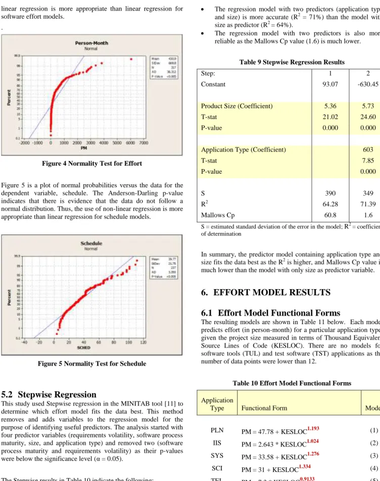
Figure 4 is a plot of normal probabilities versus the data for the dependent variable, effort. The data depart from the fitted line most evident in the extremes. The Anderson-Darling p-value indicates that, at a levels greater than 0.05, there is evidence that the data do not follow a normal distribution. Thus, the use of
non-linear regression is more appropriate than non-linear regression for software effort models.
.
Figure 4 Normality Test for Effort
Figure 5 is a plot of normal probabilities versus the data for the dependent variable, schedule. The Anderson-Darling p-value indicates that there is evidence that the data do not follow a normal distribution. Thus, the use of non-linear regression is more appropriate than linear regression for schedule models.
Figure 5 Normality Test for Schedule
5.2
Stepwise Regression
This study used Stepwise regression in the MINITAB tool [11] to determine which effort model fits the data best. This method removes and adds variables to the regression model for the purpose of identifying useful predictors. The analysis started with four predictor variables (requirements volatility, software process maturity, size, and application type) and removed two (software process maturity and requirements volatility) as their p-values were below the significance level (α = 0.05).
The Stepwise results in Table 10 indicate the following:
The regression model with two predictors (application type and size) is more accurate (R2 = 71%) than the model with size as predictor (R2 = 64%).
The regression model with two predictors is also more reliable as the Mallows Cp value (1.6) is much lower.
Table 9 Stepwise Regression Results
Step: 1 2
Constant 93.07 -630.45
Product Size (Coefficient) 5.36 5.73
T-stat 21.02 24.60
P-value 0.000 0.000
Application Type (Coefficient) 603
T-stat 7.85
P-value 0.000
S 390 349
R2 64.28 71.39
Mallows Cp 60.8 1.6
S = estimated standard deviation of the error in the model; R2 = coefficient of determination
In summary, the predictor model containing application type and size fits the data best as the R2 is higher, and Mallows Cp value is
much lower than the model with only size as predictor variable.
6.
EFFORT MODEL RESULTS
6.1
Effort Model Functional Forms
The resulting models are shown in Table 11 below. Each model predicts effort (in person-month) for a particular application type, given the project size measured in terms of Thousand Equivalent Source Lines of Code (KESLOC). There are no models for software tools (TUL) and test software (TST) applications as the number of data points were lower than 12.
Table 10 Effort Model Functional Forms
Application
Type Functional Form Model
PLN PM= 47.78 + KESLOC1.193 (1) IIS PM= 2.643 * KESLOC1.024 (2) SYS PM= 33.58 + KESLOC1.276 (3) SCI PM= 31 + KESLOC1.334 (4) TEL PM= 7.3 * KESLOC0.9133 (5) RTE PM= 60.14 + KESLOC1.442 (6)
Application
Type Functional Form Model
MP PM= 6.602 * KESLOC1.045 (7) VC PM= 9.048 * KESLOC1.018 (8) VP PM= 22.27 * KESLOC0.8049 (9) SCP PM = 26.43 * KESLOC0.8668 (10)
6.2
Effort Model Validity
Table 12 below shows the model validity results. All regression models are significant as the t-statistics exceed the two-tailed critical values, given the coefficient alpha (0.05) and degrees of freedom (DF).
Table 11 Effort Model Validity Results
Model t-statistics F-Stat N DF Intercept C Coefficient A Exponent B (1) 2.5 ** 34.1 20 18 (2) ** 5.5 23.1 535.6 16 14 (3) 3.6 ** 41.8 ** 25 23 (4) 2.7 ** 33.4 ** 17 15 (5) ** 13.4 18.0 325.5 47 45 (6) 6.9 ** 52.9 ** 57 55 (7) ** 7.2 15.2 231.1 33 31 (8) ** 11.0 17.2 296.6 27 25 (9) ** 13.8 11.7 136.0 18 16 (10) ** 21.8 18.6 345.3 37 35 DF = degrees of freedom; N = sample size
6.3
Effort Model Reliability
Table 13 shows the accuracy test results. All effort models are reliable as their MAD and CV are ≤ 40%.
Table 12 Effort Model Reliability Results Model SEE (%) MAD (%) CV (%) R 2 KESLOC (min) KESLOC (MAX) (1) 0.5 35 38 ** 10 570 (2) 0.2 18 24 97 18 417 (3) 0.5 36 43 ** 6 842 (4) 0.5 40 39 ** 2 226 (5) 0.5 35 32 88 1 532 (6) 0.5 36 39 ** 2 201 (7) 0.5 36 40 88 1 229 (8) 0.5 37 35 92 1 330 (9) 0.5 35 15 89 1 221 (10) 0.4 34 29 91 1 193 SEE = standard error of estimate; MAD = mean absolute deviation; CV = coefficient of variation; R2 = coefficient of determination; min = minimum; max = maximum
7.
SCHEDULE MODEL RESULTS
7.1
Schedule Model Functional Forms
The resulting models are shown in Table 14. Each model predicts schedule (in months) for a particular application type, given the project size (KESLOC) and staffing level (FTE). There are no models for vehicle payload, software tools and test software application types as the number of data points were lower than 10.
Table 13 Schedule Model Functional Forms
AT Functional Form Model
PLN SCHED = 2.657 * KESLOC0.9995 * FTE-0.9854 (11) IIS SCHED = 6.034 * KESLOC0.6622
* FTE-0.6002 (12) SYS SCHED = 7.681 * KESLOC0.8363
* FTE-0.9489 (13) SCI SCHED = 16.87 * KESLOC0.3082
* FTE-0.2603 (14) TEL SCHED = 14.78 * KESLOC0.4512
* FTE-0.4881 (15) RTE SCHED = 18.08 * KESLOC0.5201
* FTE-0.5695 (16) MP SCHED = 9.934 * KESLOC0.731 * FTE-0.5978 (17) VC SCHED = 8.288 * KESLOC0.8527 * FTE-0.772 (18) SCP SCHED = 30.6 * KESLOC0.4982 * FTE-0.4895 (19)
7.2
Schedule Model Validity
Table 15 shows the schedule model validity results. All regression models are significant as the t-statistics exceed the two-tailed critical values and the VIF values indicate no multicollinearity present in the analysis.
Table 14 Schedule Model Validity Results
Model t-statistics VIF N DF Coefficient A Exponent B Exponent C (11) 1.7 4.3 -4.8 5.5 10 7 (12) 4.1 5.6 -3.7 1.4 19 16 (13) 5.6 5.5 -5.1 4.2 14 11 (14) 6.1 1.5 -1.4 7.7 14 11 (15) 16.5 5.5 -6.1 4.6 42 39 (16) 16.4 7.1 -6.7 2.2 44 41
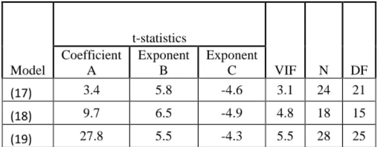
Model t-statistics VIF N DF Coefficient A Exponent B Exponent C (17) 3.4 5.8 -4.6 3.1 24 21 (18) 9.7 6.5 -4.9 4.8 18 15 (19) 27.8 5.5 -4.3 5.5 28 25
DF = degrees of freedom; N = sample size; VIF = variance inflation factor
7.3
Schedule Model Reliability
Table 16 shows the accuracy test results. All schedule models are reliable as their MAD and CV are ≤ 40%.
Table 15 Schedule Model Reliability Results Model SEE (%) MAD (%) CV (%) KESLOC (min) KESLOC (MAX) (11) 0.3 19 19 10 570 (12) 0.4 31 31 18 417 (13) 0.4 27 24 7 764 (14) 0.4 25 24 2 120 (15) 0.4 28 22 1 312 (16) 0.3 23 23 5 201 (17) 0.4 35 34 1 225 (18) 0.4 34 34 1 330 (19) 0.3 25 21 1 193
SEE = standard error of estimate; MAD = mean absolute deviation; CV = coefficient of variation; min = minimum; max = maximum
8.
CONCLUSION
8.1
Primary Findings
This study resulted in seven primary findings:
1. The Anderson-Darling test proved that nonlinear regression is more appropriate than ordinary least squares for developing both, software effort and schedule estimation models.
2. The Stepwise regression analysis revealed that software effort models based on size and application types are more accurate that models based on size alone. Size (KESLOC) alone explains 64% of the variation in effort. Size and application type explain71% of the variation in effort. 3. The regression results show that the effect of product size
and staff levels on software development schedule is significant, indicating that when KESLOC increases and/or staff level decreases, the schedule duration tends to increase.
4. All effort and schedule models were deemed valid as these did not violate any of the regression assumptions or
diagnostic tests, and met the model selection criterion in Table 5.
5. Meaningful productivity comparisons (ESLOC/PM) can be made when projects are grouped by application types. The productivity benchmarks and ranking (from lowest to highest) crosschecks with recent studies.
8.2
Challenges to Validity
Although the models were deemed reliable, they still have a few limitations:
1. A larger dataset (>400 projects) is required to increase model validity and accuracy. A future investigation should attempt to control for the impact of operating environment. 2. A non-random sample was preferred as the researcher had
access to names in the population and the selection process for participants was based on their convenience and availability. However, this process limits the ability to generalize to a population.
3. Two popular application domains were not addressed in this study -- Project Control and Training. A future investigation should attempt to collect project data for these two domains.
8.3
Future Research
The following topics may be considered for future research: 1. Develop a software effort model using functional
requirements along with application type with a similar experimental design.
2. Instead of developing multiple models, pioneer a single software effort estimating model using size, quantitative values for application type, and operating environment. 3. Use local data to calibrate COCOMO and/or SEER-SEM
using application types in lieu of application domains.
8.4
Summary
Nineteen software estimation models have been developed based on 317 programs implemented within the U.S. Department of Defense. The source data provided valuable insight into the costs and schedules associated with the vendor’s implementation team in the course of developing and implementing software.
The method is simpler and more viable to use for early estimates than traditional parametric cost models.
The productivity benchmarks (ESLOC/PM) are appropriate for validating productivity estimates.
9.
REFERENCES
[1] Boehm B., Software Engineering Economics. Englewood Cliffs, NJ, Prentice‐Hall, 1981
[2] Boehm B., Abts C., Brown W., Chulani S., Clark B., Horowitz E., Madachy R., Reifer D., Steece B., Software Cost Estimation with COCOMO II, Prentice‐Hall, 2000
[3] Boehm, B., 2000, “Safe and simple software cost analysis,”
Software, IEEE, 17(5), pp. 14–17.
[4] Clark, B., Devnani-Chulani, S., and Boehm, B., 1998, “Calibrating the COCOMO II Post-Architecture model,” Proc. Int’l Conf. Software Eng. (ICSE ’98), pp. 477–480. [5] Clark, B. K., 1997, “The Effects of Software Process
Maturity on Software Development Effort,” Technical Report No. AAT 9816016, University of Southern California, CA.
[6] Galorath, 2001, SEER-SEM™ User's Manual, Galorath, Inc., El Segundo, CA, Chaps.1-4, 6-6, 15-6.
[7] Government Accountability Office, 2009, “GAO Cost Estimating and Assessment Guide: Best Practices for Developing and Managing Capital Program Costs”
http://www.gao.gov/products/GAO-09-3SP, site accessed on 28 February 2014.
[8] IEEE, 1993, “IEEE Standard for Software Productivity Metrics,” IEEE Std 1045-1992.
[9] Liang, T., and Noore, A., 2003, “Multistage Software Estimation,” Proc. 35th Southeastern Symp. System Theory,
pp. 232–236.
[10]Maxwell, K. D., Van Wassenhove, L., and Dutta, S., 1996, “Software Development Productivity of European Space, Military, and Industrial Applications,” Software Engineering, IEEE Transactions, 22(10), pp. 706–718.
[11]Minitab Inc., 2003, MINITAB 14, www.minitab.com Site accessed in 2005 [student license purchased online] [12]Jones C., McGarry J., Dean J., Rosa W., Madachy, R.,
Boehm B., Clark B., Tan T., 2013, “Software Cost Metrics Manual” http://softwarecost.org/index.php?title=Main_Page, Site accessed on 27 February 2014.
[13] Jones, C., 2003, “Variations in Software Development Practices,” Software IEEE, pp. 22–27.
[14]Putnam, L., and Myers, W., 1991, Measures for Excellence:
Reliable Software on Time, Within Budget, Prentice Hall
PTR, Upper Saddle River, NJ, pp. 1–356.
[15]Madachy, R.; Boehm, B.; Clark, B.; Tan, T.; Rosa, W. "US DoD Application Domain Empirical Software Cost Analysis", Empirical Software Engineering and
Measurement (ESEM), 2011 International Symposium on,
On page(s): 392 - 395
[16] Lipkin, I., 2011, “Test Software Development Project Productivity Model”, Dissertation Thesis, Univerity of Toledo (Toledo, OH, 2011).
[17]Rosa W., Boehm B., Clark B., Madachy R., Dean J., 2013, “Domain-Driven Software Cost and Schedule Estimating Models: Using Software Resource Data Reports (SRDRs)”, 2013 International Cost Estimating and Analysis Association (ICEAA), Professional Development & Training Workshop [18]Rosa W., Packard T., Krupanand A., James Bilbro J., Hodal
M.: COTS integration and estimation for ERP. Journal of Systems and Software 86(2): 538-550 (2013)
[19]Software Resource Data Report, 2011,
http://dcarc.cape.osd.mil/Files/Policy/2011-SRDRFinal.pdf [20] Tan, T, “Domain‐Based Effort Distribution Model for
Software Cost Estimation,” PhD Dissertation, Computer Science Department, University of Southern California, June 2012.
[21]The International Software Benchmarking Group, 2013, www.isbsg.org, [professional license purchased online]