The ROI of Systems
Engineering: Some
Quantitative Results for
Software-Intensive Systems
Barry Boehm,1 Ricardo Valerdi, 2, * and Eric Honour31Center for Systems & Software Engineering, University of Southern California, Los Angeles, CA 90089 2Massachusetts Institute of Technology, Cambridge, MA 02139
3University of South Australia & Honourcode, Inc., Cantonment, FL 32533 ROI: SOME QUANTITATIVE RESULTS FOR SOFTWARE-INTENSIVE SYSTEMS
Received 1 August 2007; Accepted 16 December 2007, after one or more revisions Published online in Wiley InterScience (www.interscience.wiley.com)
DOI 10.1002/sys.20096
ABSTRACT
This paper presents quantitative results on the return on investment of systems engineering (SE-ROI) from an analysis of the 161 software projects in the COCOMO II database. The analysis shows that, after normalizing for the effects of other cost drivers, the cost difference between projects doing a minimal job of software systems engineering—as measured by the thorough-ness of its architecture definition and risk resolution—and projects doing a very thorough job was 18% for small projects and 92% for very large software projects as measured in lines of code. The paper also presents applications of these results to project experience in deter-mining “how much up front systems engineering is enough” for baseline versions of smaller and larger software projects, for both ROI-driven internal projects and schedule-driven outsourced systems of systems projects. © 2008 Wiley Periodicals, Inc. Syst Eng
Key words: return on investment; systems engineering measurement; COCOMO; COSYSMO; value of systems engineering; systems architecting
* Author to whom all correspondence should be addressed (e-mail: [email protected]; [email protected]; [email protected]).
Systems Engineering © 2008 Wiley Periodicals, Inc.
1. INTRODUCTION: MOTIVATION AND CONTEXT
1.1. Motivation: The Need for a Business Case for Systems Engineering Investments How much systems engineering is enough? Some deci-sion-makers draw on analogies such as, “We pay an architect 10% of the cost of a building, so that’s what we’ll pay for systems engineering.” But is 10% way too little, or way too much? Many cost-cutting decision-makers see systems engineering as an activity that doesn’t directly produce the product, and as a result try to minimize its cost. But this often leads to an increased amount of late rework and embarrassing overruns.
Despite its recognition since the 1940s, the field of systems engineering is still not as well understood as the much later field of software engineering. It is de-fined by the International Council on Systems Engi-neering [Crisp, 2005] as “an interdisciplinary approach and means to enable the realization of successful sys-tems,” with further explanation clarifying that the field “focuses on defining … required functionality early,” “integrates all disciplines and specialty groups into a team effort” with “structured development from con-cept to production to operation,” and “considers both business and technical needs.” The definition is pur-posefully vague, focusing on the thought processes, because successful systems engineering practitioners vary widely in the application of those processes. The field includes elements of both technical and manage-ment expertise—technical definition and control to ar-chitect the structures that will become the system, and management leadership to motivate and guide the inter-disciplinary effort necessary to create the system.
Despite the lack of full understanding, it is clear that systems engineering is viewed as an essential field with high value, one whose value increases significantly with the size and complexity of the development effort. Evidence for this view is contained in the high salaries and leadership roles entrusted to systems engineers. An exploration of the ontology (shared understanding) of systems engineering [Honour and Valerdi, 2006] shows the following elements are widely considered to be part of the field:
• Mission/Purpose Definition. Describing the
mis-sion and quantifying the stakeholder preferences.
• Requirements Engineering. Creation and
man-agement of requirements.
• System Architecting. Synthesizing a design for
the system in terms of its component elements and their relationships. Component elements may include software, hardware, or process.
• System Implementation. System-level efforts to
integrate the components of the first system(s) into a configuration that meets the defined mis-sion or purpose while complying with require-ments.
• Technical Analysis. Multidisciplinary analysis
focused on system emergent properties, usually used either to predict system performance or to support decision tradeoffs.
• Technical Management/Leadership. Efforts to
guide and coordinate the technical personnel to-ward the appropriate completion of technical goals, including among others formal risk man-agement.
• Scope Management. Technical definition and
management of acquisition and supply issues to ensure that a project performs only the tasks necessary.
• Verification and Validation. Proof of the system
through comparison with requirements (verifica-tion) and comparison with the intended mission (validation).
Using data from 25 years of calibration and analysis of the Constructive Cost Model (COCOMO) collection of project data, this paper explores the business case for systems engineering in terms of system architecting and risk resolution. We follow Rechtin [1991] in defining systems architecting as including many of the key ele-ments of systems engineering, including definition and validation of the system’s operational concept, require-ments, and life cycle plans.
Recent systems engineering research is beginning to quantify the value of the field [Honour and Mar, 2002]. Such quantification is one step toward better under-standing the field. In a pragmatic way, however, the quantification also seeks to provide useful tools for management decisions. Systems engineering has suf-fered from a lack of productivity measures. Because the field includes highly varied work elements, and because many of the work elements are subjective in nature, no effective productivity measures have yet been devised. As a result, the field has had decade-long cycles of acceptance and rejection. While systems engineers have been retained as technical leaders, funding of the efforts has varied widely. Research on 43 systems projects [Honour, 2004a] shows that systems engineering efforts varied from less than 1% of the project total funding to greater than 25%. Survey participants could not explain the variation, nor could they justify it. In many cases, participant emotions were raw about the quality level allowed by lower funding profiles. This research showed a distinct correlation between the systems
en-gineering effort and the cost and schedule success as shown in Figures 1 and 2.
In a more general survey [Honour, 2004b], anecdotal evidence from seven separate research efforts provided the following conclusions:
• Better technical leadership correlates to program success.
• Better/more systems engineering correlates to shorter schedules by 40% or more, even in the face of greater complexity.
• Better/more systems engineering correlates to lower development costs, by 30% or more. • Optimum level of systems engineering is about
15% of a total development program.
• Programs typically operate at about 6% systems engineering.
(See Honour [2004b] for the list of references.) Such heuristics are helpful, but fall short of the kind of information needed by a manager making budget decisions. Systems engineering needs definitive infor-mation about the levels and kinds of tasks that matter to the results of a project.
Figure 2. Schedule overrun as a function of SE effort. [Color figure can be viewed in the online issue, which is available at www.interscience.wiley.com.]
Figure 1. Cost overrun as a function of SE effort. [Color figure can be viewed in the online issue, which is available at www.interscience.wiley.com.]
INCOSE has made the determination of the return on investments in systems engineering a high-priority research topic in its Vision 2020 document [Crisp, 2005]. A partial answer to this question in the domain of software-intensive systems development is provided below.
1.2. Context: Analysis of Contributing Factors to Software Development Productivity
Most of the quantitative analyses done to date on SE-ROI have shown statistical correlations between the percentage of system development cost and develop-ment time devoted to systems engineering and the per-centage of additional cost and time needed to produce a satisfactory system. This is not a direct measure of business value or mission effectiveness, but it is a good proxy.
In general, though, the data available for these analy-ses have not included data that could help determine how much of the correlation is due to systems engineer-ing effectiveness or to other factors such as require-ments volatility, contractual budget and schedule stretchouts, domain experience, or personnel capability. The 161 software projects in the COCOMO II data-base collected over a 25-year period contain data on these attributes as part of each project’s report on 23 size, product, process, project, and personnel factors. Its attribute for systems engineering effectiveness is the degree of thoroughness of the project’s architecture definition and risk resolution by its Preliminary Design Review or equivalent, based on seven factors discussed below.
Emerging models for estimating systems engineer-ing cost and time such as COSYSMO [Valerdi, 2005] have databases including many of these attributes, but they are limited to addressing the cost aspect of ROI since they only estimate system engineering costs and not their effects on development. The cost and schedule data in the COCOMO II database include both software systems engineering and software development effort, allowing for analysis of their corresponding effect on cost.
2. FOUNDATIONS OF THE COCOMO II ARCHITECTURE AND RISK RESOLUTION (RESL) FACTOR
2.1. Experiential Origins of the RESL Factor
The original Constructive Cost Model (COCOMO) for software cost and time estimation [Boehm, 1981] did not include a factor for systems engineering
thorough-ness, or any factors reflecting management control over a project’s diseconomies of scale. The closest factor to systems engineering thoroughness was called Modern Programming Practices, which included such practices as top-down development, structured programming, and design and code inspections. Diseconomies of scale were assumed to be built into a project’s development mode: a low-criticality project had an exponent of 1.05 relating software project size to project development effort. This meant that doubling the product size in-creased effort by a factor of 2.07. A mission-critical project had an exponent of 1.20, which meant that doubling product size increased effort by a factor of 2.30.
Subsequent experience and analyses at TRW during the 1980s indicated that some sources of software de-velopment diseconomies of scale were management controllables, and that thoroughness of systems engi-neering was one of the most significant sources. For example, some large TRW software projects that did insufficient software architecture and risk resolution had very high rework costs [Boehm, 2000], while simi-lar smaller projects had smaller rework costs.
2.1.1. Reducing Software Rework via Architecture and Risk Resolution
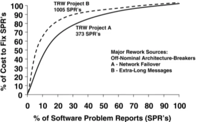
Analysis of project defect tracking cost-to-fix data (a major source of rework costs) showed that 20% of the defects accounted for 80% of the rework costs, and that these 20% were primarily due to inadequate architec-ture definition and risk resolution.
For example, in TRW Project A in Figure 3, most of the rework was the result of development of the network operating system to a nominal-case architecture, and finding that the systems engineering of the architecture neglected to address the risk that the operating system architecture would not support the project requirements of successful system fail-over if one or more of the
processors in the network failed to function. Once this was discovered during system test, it turned out to be an “architecture-breaker” causing several sources of expensive rework to the already-developed software. A similar “architecture-breaker,” the requirement to han-dle extra-long messages (over 1 million characters), was the cause of most of the rework in Project B, whose original nominal-case architecture assumed that almost all messages would be short and easy to handle with a fully packet-switched network architecture.
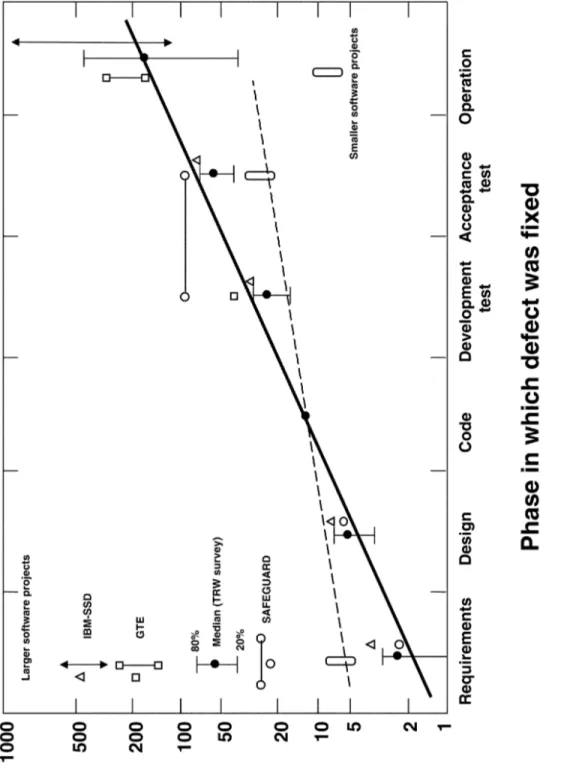
Earlier, analyses of cost-to-fix data at IBM [Fagan 1976], GTE [Daly 1977], Bell Labs [Stephenson 1976], and TRW [Boehm 1976] found consistent results show-ing the high payoff of findshow-ing and fixshow-ing defects as early as possible. As seen in Figure 4, relative to an effort of 10 units to fix a requirements defect in the Code phase, fixing it in the Requirements phase involved only about 2 units of effort, while fixing it in the Operations phase involved about 100 units of effort, sometimes going as high as 800 units. These results caused TRW to develop policies requiring thorough risk analyses of all require-ments by the project’s Preliminary Design Review (PDR). With TRW’s adoption of the Ada programming language and associated ability to verify the consis-tency of Ada module specifications, the risk policy was extended into an Ada Process Model for software, also requiring that the software architecture pass an Ada compiler module consistency check prior to PDR [Royce, 1998].
2.1.2. A Successful Example: CCPDS-R
The apparent benefits of fixing requirements at early phases of the life cycle motivated subsequent projects to perform much of systems integration before provid-ing the module specifications to programmers for cod-ing and unit test. As a result of this and the elimination of architecture risks prior to Preliminary Design Re-view, subsequent projects were able to significantly reduce late architecture-breaker rework and the steep slope of the cost-to-fix curve. A good example was the Command Center Processing and Display System-Re-placement (CCPDS-R) project described in Royce [1998], whose flattened cost-to-fix curve is shown in Figure 5. It delivered over a million lines of Ada code within its original budget and schedule. Its PDR was held in month 14 of a 35-month initial-delivery sched-ule and included about 25% of the initial-delivery budget, including development and validation of its working high-risk software, such as its network operat-ing system and the key portions of its user interface software.
2.2. The RESL Factor in Ada COCOMO and COCOMO II
The flattened cost-to-fix curve for large projects exem-plified in Figure 5 confirmed that increased emphasis on architecture and risk resolution led to reduced re-work and diseconomies of scale on large projects. In 1987–1989, TRW developed a version of COCOMO for large mission-critical projects using the Ada Process model, called Ada COCOMO [Boehm and Royce, 1989]. It reduced the 1.20 exponent relating product size to project effort as a function of the degree that the project could follow the Ada Process model. This was difficult to do on some projects required by government standards and contracts to use sequential waterfall-model processes. Thus, it made reduction of software project diseconomies of scale via architecture and risk resolution operate as a management controllable factor, and helped government and industry people evolve toward more risk-driven concurrently engineered proc-esses rather than documentation-driven procproc-esses.
2.2.1. Resulting Risk-Driven Concurrent Engineering Software Process Models
The Ada Process Model and the CCPDS-R project showed that it was possible to reinterpret sequential waterfall process model phases, milestones, and re-views to enable projects to perform risk-driven concur-rent engineering of their requirements, architecture, and plans, and to apply review criteria focusing on the compatibility and feasibility of these artifacts.
Subsequently, these practices were elaborated into general software engineering—and systems engineer-ing for software-intensive systems—process models emphasizing risk-driven concurrent engineering and associated milestone review pass-fail criteria. These included the Rational Unified Process [Royce, 1998; Jacobson, Booch, and Rumbaugh, 1999; Rumbaugh, Jacobson, and Booch, 2004; Kruchten, 2000], and the USC Model-Based (System) Architecting and Software Engineering (MBASE) model [Boehm and Port, 1999, 2001], which integrated the risk-driven concurrent en-gineering spiral model [Boehm et al., 1998] with the Rechtin concurrent engineering Systems Architecting approach [Rechtin, 1991; Rechtin and Maier, 1997]. Both RUP and MBASE used a set of anchor point milestones, including the Life Cycle Objectives (LCO) and Life Cycle Architecture (LCA) as their model phase gates. Actually, these were determined in a series of workshops involving the USC Center for Software En-gineering and its 30 government and industry affiliates, including Rational, Inc., as phase boundaries for CO-COMO II cost and schedule estimates [Boehm, 1996]. Table I summarizes the pass/fail criteria for the LCO and LCA anchor point milestones.
Figur e 4. Risk of d elaying risk ma n agement.
More recently, the MBASE approach has been ex-tended into an Incremental Commitment Model (ICM) for overall systems engineering. It uses the anchor point milestones and feasibility rationales to synchronize and stabilize the concurrent engineering of the hardware, software, and human factors aspects of a system’s ar-chitecture, requirements, operational concept, plans, and business case [Pew and Mavor, 2007; Boehm and Lane, 2007]. A strong feasibility rationale will include results of architecture tradeoff and feasibility analyses such as those discussed in [Clements, Kazman, and Klein, 2002] and [Maranzano et al., 2005].
2.2.2. The RESL Factor in COCOMO II
The definition of the COCOMO II software cost esti-mation model [Boehm et al., 2000] was evolved during 1995–1997 by USC and its 30 industry and government affiliates. Its diseconomy-of-scale factor is a function of RESL and four other scale factors, two of which are also management controllables: Capability Maturity Model maturity level and developer-customer-user team cohesion. The remaining two are Precedentedness and Development Flexibility. The definition of the RESL rating scale was elaborated into the seven con-tributing factors shown in Table II. As indicated in Table I, “architecture and risk resolution” includes the
current engineering of the system’s operational con-cept, requirements, plans, business case, and feasibility rationale as well as its architecture, thus covering most of the key elements that are part of the systems engi-neering function.
The values of the rating scale for the third charac-teristic, percent of development schedule devoted to establishing architecture, were obtained through a be-havioral assessment of the range of possible values that systems engineers might face. The minimum expected level of effort spent on architecting was assumed to be 5%, or 1/20, of the total project effort. To operationalize the remaining rating levels, a similar logic was applied. It was assumed that the subsequent rating levels were 10% (1/10), 17% (1/6), 25% (1/4), or 33% (1/3) of the project effort. In the best case, 40% or more effort would be invested in architecting.
Each project contributing data to the COCOMO II database used Table II as a guide for rating its RESL factor. The ratings for each row could have equal or unequal weights as discussed between data contributors and COCOMO II researchers in data collection ses-sions. The distribution of RESL factor ratings of the 161 projects in the COCOMO II database is approximately a normal distribution, as shown in Figure 6.
Table I. Anchor Point Milestone Pass/Fail Feasibility Rationales
The contribution of a project’s RESL rating to its diseconomy of scale factor was determined by a Bayesian combination of expert judgment and a multi-ple regression analysis of the 161 representative
soft-ware development projects’ size, effort, and cost driver ratings in the COCOMO II database. These include commercial information technology applications, elec-tronic services, telecommunications, middleware, engi-neering and science, command and control, and real time process control software projects. Their sizes range from 2.6 thousand equivalent source lines of code (KSLOC) to 1300 (KSLOC), with 13 projects below 10 KSLOC and 5 projects above 1000 KSLOC. Equivalent lines of code account for the software’s degrees of reuse and requirements volatility.
The expert-judgment means and standard deviations of the COCOMO II cost driver parameters were treated
as a priori knowledge in the Bayesian calibration, and
the corresponding means and standard deviations re-sulting from the multiple regression analysis of the historical data were treated as an a posteriori update of the parameter values. The Bayesian approach produces a weighted average of the expert and historical data
Figure 6. RESL ratings for 161 projects in the COCOMO database.
values, which gives higher weights to parameter values with smaller standard deviations. The detailed approach and formulas are provided in Chapter 4 of the CO-COMO II text [Boehm et al., 2000].
2.2.3. RESL Calibration Results
Calibrating the RESL scale factor was a test of the hypothesis that proceeding into software development with inadequate architecture and risk resolution results (i.e., inadequate systems engineering results) would cause project effort to increase due to the software rework necessary to overcome the architecture deficien-cies and to resolve the risks late in the development cycle—and that the rework cost increase percentage would be larger for larger projects.
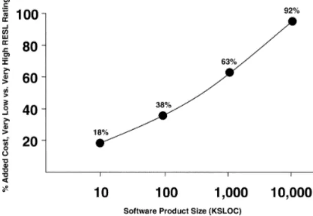
The regression analysis to calibrate the RESL factor and the other 22 COCOMO II cost drivers confirmed this hypothesis with a statistically significant result. The calibration results determined that for this sample of 161 projects, the difference between a Very Low RESL rating and an Extra High rating was an extra contribu-tion of 0.0707 added to the exponent relating project effort to product size. This translates to an extra 18% effort for a small 10 KSLOC project, and an extra 92% effort for an extra-large 10,000 KSLOC project.
Figure 7 summarizes the results of the analysis. It shows that at least for this sample of 161 software projects, the difference between a project doing a mini-mal job of systems engineering—as measured by its degree of architecture and risk resolution—is an in-creasingly large increase in overall project effort and cost, independent of the effects of the other 22 CO-COMO II cost drivers. This independence is because the regression analysis also accounts for variations in effort due to the other 22 factors in its statistical results. The level of statistical significance of the RESL pa-rameter was above 1.96 which is the critical value for
the analysis of 23 variable and 161 data points as shown in the Appendix. Moreover, the pairwise correlation analysis shows that no variable was correlated more than 0.4 with RESL.
3. RESULTING ROI FOR SOFTWARE SYSTEMS ENGINEERING IMPROVEMENT INVESTMENTS
Investing in improved software systems engineering involves a higher and stronger level and focus of effort on risk-driven concurrent engineering of software sys-tem requirements, architecture, plans, budgets, and schedules. It also requires assurance of their consis-tency and feasibility via prototyping, modeling, analy-sis, and success-critical stakeholder review and commitment to support the next phase of project activ-ity, as discussed at the end of section 2.1.
The results of the COCOMO II calibration of the RESL factor shown in Figure 7 enable us to determine the ROI for such investments, in terms of the added effort required for architecture and risk resolution, and the resulting savings for various sizes of software sys-tems measured in KSLOC. A summary of these results is provided in Table III for a range of software system sizes from 10 to 10,000 KSLOC.
The percentage of time invested in architecting is provided for each RESL rating level together with:
• Level of effort. The numbers reflect the fraction of the average project staff level on the job doing systems engineering if the project focuses on systems engineering before proceeding into de-velopment for 5%, 10%, 17%, etc. of its planned schedule; it looks roughly like a Rayleigh curve observed in the early phases of software projects [Boehm, 1981].
• RESL investment cost %. The percent of pro-posed budget allocated to architecture and risk resolution. This is calculated by multiplying the RESL percentage calendar time invested by the fraction of the average level of project staffing incurred for each rating level. For example, the RESL investment cost for the Very Low case is calculated as: 5 ∗ 0.3 = 1.5.
• Incremental investment. The difference between the RESL investment cost % of the nth rating level minus the (n – 1)th level. The incremental investment for the Low case is calculated as: 4 – 1.5 = 2.5%.
• Scale factor exponent for rework effort. The ex-ponential effect of the RESL driver on software project effort as calibrated from 161 projects.
Figure 7. Added cost of minimal software systems engi-neering.
Return on Investment values are calculated for five different rating scale levels across four different size systems through the calculation of:
• Added effort. Calculated by applying the scale factor exponent for rework (i.e., 1.0707) to the size of the system (i.e., 10 KSLOC) and calculat-ing the added effort introduced. For the 10 KSLOC project, the added effort for the Very Low case is calculated as follows:
Added effort =10
1.0707− 10
10 ∗ 100
= 17.7.
• Incremental benefit. The difference between the added effort for the nth case and the (n – 1)th case. The incremental benefit for the Low case is cal-culated as: 17.7 – 13.9 = 3.8.
• Incremental cost. Same as the value for incre-mental investment.
• Incremental ROI. Calculated as difference be-tween the benefit and the cost divided by the cost. For the 10 KSLOC project, the incremental ROI for the Low case is calculated as follows:
ROI =(3.8 − 2.5) 2.5
= 0.52.
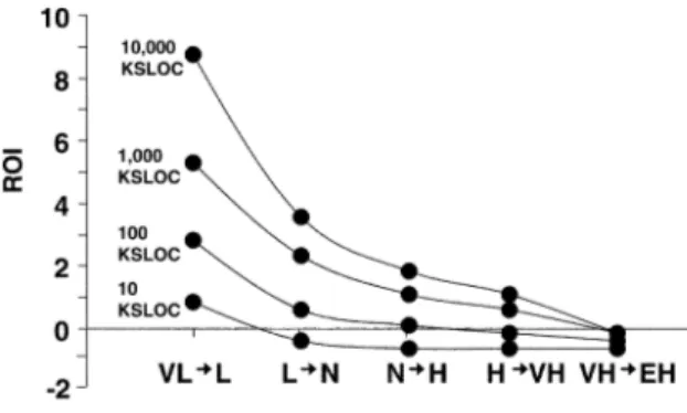
It is evident that architecting has a decreasing amount of incremental ROI as a function of RESL effort invested. Larger projects enjoy higher levels of ROI, which supports the idea that the point of diminishing returns (negative incremental ROI) is dependent on the size of the system. These results are presented graphi-cally in Figure 8.
4. DETERMINING “HOW MUCH ARCHITECTING IS ENOUGH”
The results above can also be used in the increasingly frequent situation of determining “how much architect-ing is enough” for schedule-driven software-intensive systems projects involving outsourcing. Frequently, such projects are in a hurry to get the suppliers on the job, and spend an inadequate amount of time in system architecture and risk resolution before putting supplier plans and specifications into their Requests for Propos-als (RFPs). As a result, the suppliers will frequently deliver incompatible components, and any earlier schedule savings will turn into schedule overruns due
to rework, especially as shown above for larger projects. On the other hand, if the project spends too much time on system architecting and risk resolution, not enough time is available for the suppliers to develop their sys-tem components. This section shows how the CO-COMO II RESL factor results can be used to determine an adequate architecting “sweet spot” for various sizes of projects.
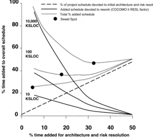
The full set of effects for each of the RESL rating levels and corresponding architecting investment per-centages are shown in Table IV for projects of size 10, 100, and 10,000 KSLOC. Also shown are the corre-sponding total-delay-in-delivery percentages, obtained by adding the architecting investment time to the re-work time, assuming constant team size during rere-work to translate added effort into added schedule. Thus, in the bottom two rows of Table IV, we can see the added investments in architecture definition and risk resolu-tion are more than repaid by savings in rework time for a 10,000 KSLOC project up to an investment of 33%, after which the total delay percentage increases.
This identifies the minimum-delay architecting in-vestment “sweet spot” for a 10,000 KSLOC project to be around 33%. Figure 9 shows the results of Table IV graphically. It indicates that for a 10,000 KSLOC pro-ject, the sweet spot is actually a flat region around a 37% architecting investment. For a 100 KSLOC project, the sweet spot is a flat region around 20%. For a 10 KSLOC project, the sweet spot is at around 5% investment in architecting. The term “architecting” is adapted from Rechtin’s System Architecting book [Rechtin, 1991], to include the overall concurrent effort involved in devel-oping and documenting a system’s operational concept, requirements, architecture, life-cycle plan, and result-ing feasibility rationale. Thus, the results in Table IV and Figure 9 confirm that investments in architecting
Table IV. Effect of Architecting Investment Level on Total Project Delay
are less valuable for small projects, but increasingly necessary as the project size increases.
However, the values and sweet spot locations pre-sented are for nominal values of the other COCOMO II cost drivers and scale factors. Projects in different situ-ations will find that “their mileage may vary.” For example, a 10 KSLOC safety-critical project—with a corresponding Very High RESL rating—will find that its sweet spot will be upwards and to the right of the nominal case 10 KSLOC sweet spot. A 10,000 KSLOC highly volatile project—with a corresponding Require-ments Volatility factor of 50%—will find that its sweet spot will be higher and to the left of the nominal case 10,000 KSLOC sweet spot, due to costs of require-ments, architecture, and other product rework. Also, various other factors can affect the probability and size of loss associated with the RESL factor, such as staff capabilities, tool support, and technology uncertainties [Boehm et al., 2000]. And these tradeoffs are only considering project delivery time and productivity and not the effects of delivered system shortfalls on business value, which would push the sweet spot for safety-criti-cal projects even further to the right.
5. CONCLUSIONS
There is little doubt that doing the right amount of systems engineering has value. To date, the difficulty has been to determine how much value. Better under-standing of the field requires that the effect of systems engineering tasks be quantified. Such quantification assists managers to set appropriate budgets, and it as-sists practitioners to select the appropriate tasks for a project of given characteristics.
Evidence has been provided for the return on invest-ment for systems engineering in the context of soft-ware-intensive systems. While the numbers may be different for non-software-intensive systems, we feel that the general framework provides significant evi-dence that larger systems enjoy larger systems engi-neering ROI values compared to smaller systems and that the most cost-effective amount of systems engi-neering has an inherent sweet spot based on the size of the system.
In this review of data from 25 years of COCOMO software projects, the ROI of some systems engineering tasks is quantified. The RESL parameter added in CO-COMO II specifically addresses the degree to which a software project achieves (or has plans and resources to achieve) a thoroughly defined architecture package (also including its operational concept, requirements, and plans) along with risks properly identified and managed, all of which are major characteristics of the systems engineering effort that defines the software. The calibration of the RESL parameter provides data about the ROI of that systems engineering effort that is based on 161 project submissions.
Therefore, in relation to the RESL systems engineer-ing efforts (architectengineer-ing and risk reduction) as used in software development projects, the data indicates the following important conclusions:
• Inclusion of greater RESL effort can improve the software productivity by factors from 18% (small software projects) to 92% (very large software projects).
• Incremental addition of greater RESL effort can result in cost ROI of up to 8:1. The greatest ROI occurs when very large software projects using Very Low RESL effort (5% of project time, 1.5% of project cost) move to somewhat greater effort. • In some cases, incremental addition of greater RESL effort is counterindicated. This is particu-larly true for small software projects that are already using in excess of 15% RESL effort. • For schedule-driven projects, optimum RESL
ef-fort varies from 10% of project time (small soft-ware projects) to 37% of project time (very large software projects).
These results strengthen the argument for the value of systems engineering by providing quantitative evi-dence that doing a minimal job of software systems engineering significantly reduces project productivity. Even higher ROIs would result from including the potential operational problems in business or mission cost, schedule, and performance that could surface as a result of inadequate systems architecting and risk reso-lution.
REFERENCES
B. Boehm, Software engineering, IEEE Trans Comput C-25 (12) (December 1976), 1226–1241.
B. Boehm, Software engineering economics, Prentice-Hall, Upper Saddle River, NJ, 1981.
B. Boehm, Anchoring the software process, Software 13(4) (July 1996), 73–82.
B. Boehm, Unifying software engineering and systems engi-neering, Computer 33(3) (March 2000), 114–116. B. Boehm and J. Lane, Using the incremental commitment
model to integrate system acquisition, systems engineer-ing, and software engineerengineer-ing, CrossTalk 20(10) (October 2007), 4–9.
B. Boehm and D. Port, Escaping the software tar pit: Model clashes and how to avoid them, ACM Software Eng Notes 24(1) (January 1999), 36–48.
B. Boehm and D. Port, Balancing discipline and flexibility with the spiral model and MBASE, CrossTalk 14(12) (December 2001), 23–28.
B. Boehm and W. Royce, Ada COCOMO and the Ada process model, Proc 5th COCOMO User’s Group, 1989, Software Engineering Institute, Pittsburgh, PA.
B. Boehm, C. Abts, A.W. Brown, S. Chulani, B.K. Clark, E. Horowitz, R. Madachy, D. Reifer, and B. Steece, Software cost estimation with COCOMO II, Prentice-Hall, Upper Saddle River, NJ, 2000.
B. Boehm, A. Egyed, Kwan, D. Port, A. Shah, and R. Madachy, Using the WinWin spiral model: A case study, IEEE Comput 31(7) (July 1998), 33–44.
P. Clements, R. Kazman, and M. Klein, Evaluating software architectures, Addison Wesley Professional, Boston, MA, 2002.
H.E. Crisp (Editor), Systems engineering vision 2020—Ver-sion 1.5, International Council on Systems Engineering, Seattle, WA, 2005.
E. Daly, Management of software engineering, IEEE Trans SW Eng SE-3 (3) (May 1977), 229–242.
M. Fagan, Design and code inspections to reduce errors in program development, IBM Syst J 15(3) (1976), 182–211. E.C. Honour, Understanding the value of systems
engineer-ing, INCOSE Int Symp, Toulouse, France, 2004a. E.C. Honour, Value of systems engineering, Cambridge, MA,
2004b.
E.C. Honour and B. Mar, Value of systems engineering—SE-COE research project progress report, INCOSE Int Symp, Las Vegas, NV, 2002.
E.C. Honour and R. Valerdi, Advancing an ontology for systems engineering to allow consistent measurement, Conf Syst Eng Res, Los Angeles, CA, 2006.
I. Jacobson, G. Booch, and J. Rumbaugh, The unified soft-ware development process, Addison-Wesley, Reading, MA, 1999.
P. Kruchten, The rational unified process: An introduction, Addison-Wesley, Reading, MA, 2000.
J.F. Maranzano, S.A. Rozsypal, G.H. Zimmerman, G.W. Warnken, P.E. Wirth, and D.W. Weiss, Architecture re-views: practice and experience, Software (March/April 2005), 34–43.
R. Pew and A. Mavor (Editors), Human-system integration in the system development process, National Academies Press, Pew & Mavor, Washington, D.C., 2007.
E. Rechtin, Systems architecting, Prentice-Hall, Englewood Cliffs, NJ, 1991.
E. Rechtin and M. Maier, The art of systems architecting, CRC Press, Boca Raton, FL, 1997.
W. Royce, Software project management: A unified frame-work, Addison Wesley, Reading, MA, 1998.
J. Rumbaugh, I. Jacobson, and G. Booch, Unified modeling language reference manual, Addison-Wesley, Reading, MA, 2004.
W. Stephenson, An analysis of the resources used in safeguard software system development, Bell Labs draft paper, Mur-ray Hill, NJ, August 1976.
R. Valerdi, The constructive systems engineering cost model (COSYSMO), PhD Dissertation, University of Southern California, 2005.
Barry Boehm is the TRW professor of software engineering and director of the Center for Systems and Software Engineering at the University of Southern California. He was previously in software engineering, systems engineering, and management positions at General Dynamics, Rand Corp., TRW, and the Defense Advanced Research Projects Agency, where he managed the acquisition of more than $1 billion worth of advanced information technology systems. Dr. Boehm originated the spiral model, the Constructive Cost Model, and the stakeholder win-win approach to software management and requirements negotiation. He is a Fellow of INCOSE.
Ricardo Valerdi is a Research Associate at the Lean Advancement Initiative at MIT and a Visiting Associate at the Center for Systems and Software Engineering at USC. He earned his BS in Electrical Engineering from the University of San Diego, MS and PhD in Industrial and Systems Engineering from USC. He is a Senior Member of the Technical Staff at the Aerospace Corporation in the Economic & Market Analysis Center. Previously, he worked as a Systems Engineer at Motorola and at General Instrument Corporation. He is on the Board of Directors of INCOSE.
Eric Honour was the 1997 INCOSE President. He has a BSSE from the US Naval Academy and MSEE from the US Naval Postgraduate School, with 37 years of systems experience. He is currently a doctoral candidate at the University of South Australia (UniSA). He was the founding President of the Space Coast Chapter of INCOSE, the founding chair of the INCOSE Technical Board, and a past director of the Systems Engineering Center of Excellence. Mr. Honour provides technical management support and systems engineering training as President of Honourcode, Inc., while continuing research into the quantification of systems engineering.
![Figure 2. Schedule overrun as a function of SE effort. [Color figure can be viewed in the online issue, which is available at www.interscience.wiley.com.]](https://thumb-us.123doks.com/thumbv2/123dok_us/657409.2579255/3.918.235.692.106.408/figure-schedule-overrun-function-effort-color-available-interscience.webp)
![Figure 5. Reducing software cost-to-fix: CCPDS-R (adapted from Royce [1998]).](https://thumb-us.123doks.com/thumbv2/123dok_us/657409.2579255/7.918.218.711.113.293/figure-reducing-software-cost-fix-ccpds-adapted-royce.webp)