A comparison of multiple testing adjustment
methods with block-correlation
positively-dependent tests
John R. Stevens1*, Abdullah Al Masud1,2, Anvar Suyundikov1,3
1 Department of Mathematics and Statistics, Utah State University, 3900 Old Main Hill, Logan, UT
84322-3900, United States of America, 2 Department of Biostatistics, Indiana University Fairbanks School of Public Health and Indiana University School of Medicine, Indianapolis, IN 46202, United States of America, 3 BioStat Solutions, Inc., 5280 Corporate Drive, Suite C200, Frederick, MD 21703, United States of America
Abstract
In high dimensional data analysis (such as gene expression, spatial epidemiology, or brain imaging studies), we often test thousands or more hypotheses simultaneously. As the num-ber of tests increases, the chance of observing some statistically significant tests is very high even when all null hypotheses are true. Consequently, we could reach incorrect conclu-sions regarding the hypotheses. Researchers frequently use multiplicity adjustment meth-ods to control type I error rates—primarily the family-wise error rate (FWER) or the false discovery rate (FDR)—while still desiring high statistical power. In practice, such studies may have dependent test statistics (or p-values) as tests can be dependent on each other. However, some commonly-used multiplicity adjustment methods assume independent tests. We perform a simulation study comparing several of the most common adjustment methods involved in multiple hypothesis testing, under varying degrees of block-correlation positive dependence among tests.
Introduction
A common initial question in a genomic study is to identify genes whose expression levels change with the different levels of some variable of interest such as a covariate or response vari-able. The response variable could be a clinical outcome or survival time, whereas the covariate could be the dose of a drug, time, treatment/control group, and so forth [1]. Questions in spa-tial epidemiology can involve identifying locations where disease risk is associated with an environmental variable [2]. Brain imaging studies can involve identifying voxels (essentially very specific brain regions) that exhibit different levels of brain activity in response to some stimulus [3,4]. These three fields (genomics, spatial epidemiology, and brain imaging), among many other fields, all can involve situations where potentially thousands (or more) features (genes, locations, voxels) are tested for differential abundance (expression, risk, brain activity) between levels of some variable of interest.
a1111111111 a1111111111 a1111111111 a1111111111 a1111111111 OPEN ACCESS
Citation: Stevens JR, Al Masud A, Suyundikov A (2017) A comparison of multiple testing adjustment methods with block-correlation positively-dependent tests. PLoS ONE 12(4): e0176124.https://doi.org/10.1371/journal. pone.0176124
Editor: Dmitri Zaykin, National Institute of Environmental Health Sciences, UNITED STATES Received: June 30, 2016
Accepted: April 5, 2017 Published: April 28, 2017
Copyright:©2017 Stevens et al. This is an open access article distributed under the terms of the Creative Commons Attribution License, which permits unrestricted use, distribution, and reproduction in any medium, provided the original author and source are credited.
Data Availability Statement: Data are generated using R code provided in the Supporting Information S2 File.
Funding: This research was supported (in the form of salaries and conference travel for two authors – JRS, AAM) by the Utah Agricultural Experiment Station (UAES), Utah State University, and approved as journal paper number 8986. During later stages of the work, BioStat Solutions, Inc. provided support in the form of salary for one author (AS). Neither of these two funders had any
Multiple hypothesis testing is often applied to identify differentially abundant features across different levels of the variable of interest. The null hypothesis for each feature is that the abundance levels are not associated with the variable of interest. With thousands (or more) of null hypotheses to test, it becomes important to control the overall type I error rate at levelα while maintaining the desired statistical power (= 1—type II error rate). Because of the mixture of true and false null hypotheses, the obtained p-values follow different types of distributions, for example Beta distributions instead of the Uniform distribution (which would result if all null hypotheses were true). Multiple comparison adjustment methods can control the FWER, FDR [5], or positive false discovery rate (pFDR) [6]. In higher-dimensional studies, most often controlling the FDR, or the pFDR, ensures more statistical power than controlling the FWER [1].
Some commonly-used multiple testing adjustment methods (such as the original FDR method by Benjamini and Hochberg (1995) [5]) assume independence of tests, which in gene expression studies translates to a questionable assumption that all genes operate indepen-dently. (Corresponding and similarly questionable assumptions in other fields would be the independence of spatial locations, or the independence of different regions of the brain.) Other multiple testing adjustment methods claim to provide error rate control under certain (or even arbitrary) dependence types among test results [7,8]. It would be useful to know how various adjustment methods perform under various levels of test dependence. The objective of this paper is to make such an evaluation so that a methodological recommendation can be made, leading to better-justified conclusions from high-dimensional data analysis. The paper is arranged in the following manner: first, in the “Methods: controlling the error rates” Section (and greater detail in Section A ofS1 File) we summarize several procedures in the literature to control error rates in multiple comparisons. Then in the “Methods: simulation analysis” Sec-tion we propose a simulaSec-tion framework and analyze several multiple comparison procedures using simulation data sets. Finally in the “Results and Discussion” Section, we finish with some observations and recommendations.
Methods: Controlling the error rates
Many multiple testing adjustment methods exist for controlling error rates. For our current purposes, we focus on several that are most commonly used and widely available to applied researchers. To ensure the main body of this article focuses on our novel contributions, we have summarized in Section A ofS1 Filethe background literature on these methods, as well as a brief discussion on dependence structures. For control of the FWER, we consider the Bon-ferroni procedure [9], Sˇida´k’s single step and step-down procedures [10,11], the Holm proce-dure [12], the Hommel procedure [13], and the Hochberg procedure [14,15]. For control of the FDR, we consider the Benjamini and Hochberg procedure [5], the Benjamini and Yekutieli procedure [7], the adaptive Benjamini and Hochberg procedure [16], the two stage Benjamini and Hochberg procedure [17], the q-value method [6], and the principal factor approximation method [8]. The multiple comparison procedures discussed in Section A ofS1 Fileare shown inTable 1. These procedures are used to adjust p-values in our simulation analysis in the “Methods: simulation analysis” Section and to visualize results in the “Results and Discussion” Section.
Methods: Simulation analysis
In this section we evaluate the performance of the multiple testing procedures from the “Meth-ods: controlling the error rates” Section (and Section A ofS1 File), under various dependence scenarios using simulated data sets. We simulatedmtest statistics (corresponding tomfeatures
role in the study design, data collection and analysis, decision to publish, or preparation of the manuscript. Specific roles of all authors are articulated in the ‘author contributions’ section. Competing interests: During the preparation of this work, one author (AS) was employed by BioStat Solutions, Inc. (see funding statement), but that author’s involvement in this work was done on their own time, and outside of their employment responsibilities. This does not alter our adherence to PLOS ONE policies on sharing data and materials.
in a hypothetical study) asZ Nðm
;SÞ. Herem is a lengthmvector of the expected
differ-ences for each test; in the high-dimensional study context,μiis the true magnitude of
differen-tial abundance for featurei. We considered two levels ofm: 2000 (where the control of the FDR would generally be more meaningful) and 100 (where control of the FWER would gener-ally be more meaningful). Our scenario of dependent test statistics (and subsequent p-values) is represented in the covariance matrix (S
), where we considered different numbers of
corre-lated tests (or features) and varying levels of correlation. In addition, we considered different sizes ofμiin order to compare the performance of these multiple comparison procedures. Our
general hypothesis is constructed as follows:
H0
i :mi¼0vs H
1
i :mi 6¼0 for i¼1;2;. . .;m:
In our study the first and the most important dependency scenarios are represented in the covariance matrix (S
mm) of test statistics (Z). Thus, the construction ofSaddresses two
issues: (1) number of total correlatedZ(corresponding to features) and (2) correlation value (ρ) of dependentZ. Regarding the first issue, our main motivation is to examine the perfor-mance of various multiple comparison procedures when increasing the total number of corre-latedZ. We considered two different total numbers of correlatedZ: 120 and 360 (out of 2000 total) for FDR control; 18 and 36 (out of 100 total) for FWER control. We also considered these dependent test statistics in blocks in order to distribute the number of dependentZ into six disjoint but equal-sized sets of correlated tests. For example, in the case of 120 dependent tests, we have six blocks, each with twenty dependentZ. In each case, the dependentZof the first three blocks were always associated with the alternative hypothesis being true (μi6¼0),
while the dependentZof the remaining three blocks were associated with the null hypothesis being true (μi= 0). Then, we set all remaining test statistics to be independent. Therefore, the
diagonal elements of the entireS
mmmatrix consist of six blocks with the remaining diagonal
elements being ones, and the off-diagonal elements being zeros. So all blocks under a specific total number of correlatedZ always appear at diagonal positions of the entireS
matrix.
Indeed, each block is a symmetric matrix inside theS
matrix.
As off-diagonal elements of the blocks on the diagonal ofS
, we considered correlation
coef-ficient valuesρ2{0, .2, .4, .6, .8, .99}. The values ofρare chosen to represent a reasonable
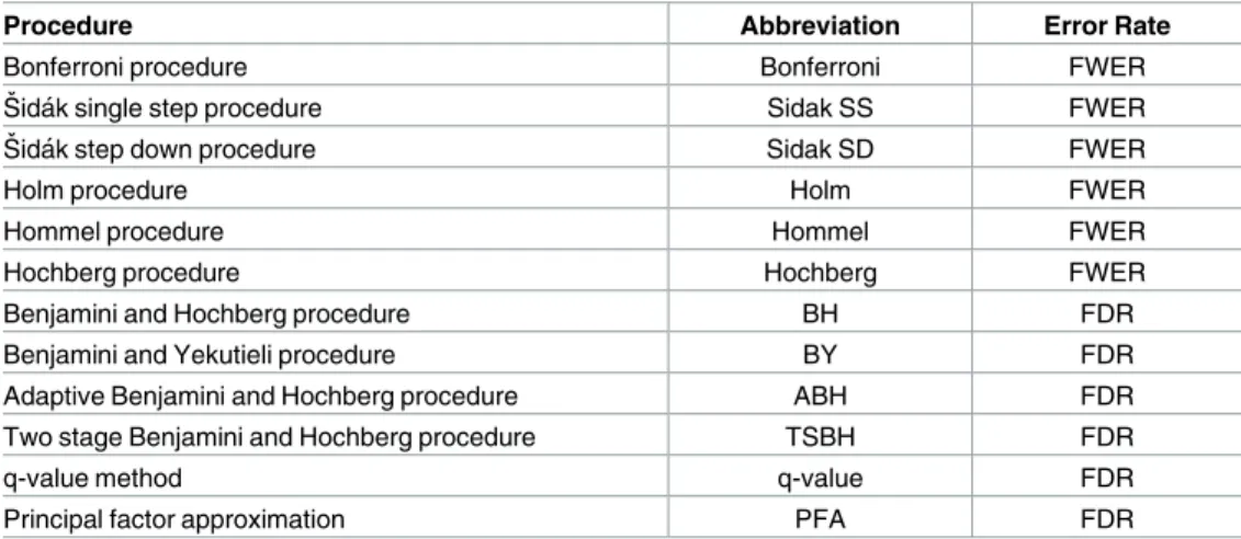
Table 1. Abbreviations of multiple comparison procedures (and their corresponding controlled error rate), used in the text and in summary figures.
Procedure Abbreviation Error Rate
Bonferroni procedure Bonferroni FWER
Sˇ ida´k single step procedure Sidak SS FWER
Sˇ ida´k step down procedure Sidak SD FWER
Holm procedure Holm FWER
Hommel procedure Hommel FWER
Hochberg procedure Hochberg FWER
Benjamini and Hochberg procedure BH FDR
Benjamini and Yekutieli procedure BY FDR
Adaptive Benjamini and Hochberg procedure ABH FDR
Two stage Benjamini and Hochberg procedure TSBH FDR
q-value method q-value FDR
Principal factor approximation PFA FDR
range of values. Non-negativeρensures that the covariance amongZis always non-negative. Thus, with such GaussianZwith positive correlation, we satisfy the condition of positive regression dependency [18] (see “Dependence among test results: PRDS and MTP2” in Section
A ofS1 File). These correlation values measure how much the dependentZ
are correlated with
each other. Specifically,ρ= 0 indicates features are completely independent; in contrast,ρ= 0.99 indicates that the linear association between features’ test statistics is almost exact. Con-sidering this block-correlation dependence structure, it helps to compare the performance of various multiple comparison procedures under the same degree of dependency in the same number of both true null and false null hypotheses. By changing theρvalues we obtain differ-ent off-diagonal elemdiffer-ents in the blocks. Thus, we summarize the construction of our general
S
mmmatrix in such a way so that, under a given number of correlatedZ, all blocks (or
sym-metrical sub-matrices) appear along the diagonal of theS
matrix, and the off-diagonal
ele-ments of the blocks preserve the degree of dependency of correlatedZ
. The following is the
general form of ourS
mmmatrix: S ¼ 1 r r 1 2 6 4 3 7 5 0 0 0 0 1 r r 1 2 6 4 3 7 5 0 0 0 0 1 r r 1 2 6 4 3 7 5 0 0 0 0 1 2 6 6 6 6 6 6 6 6 6 6 6 6 6 6 6 6 6 6 6 6 6 6 6 6 6 6 6 6 6 4 3 7 7 7 7 7 7 7 7 7 7 7 7 7 7 7 7 7 7 7 7 7 7 7 7 7 7 7 7 7 5 ð1Þ
This block-diagonal structure of theS
matrix affects the construction of our mean vectorm
for ourZ. For tests with a true null hypothesis,μi= 0, while for tests with a false null
hypothe-sis, we setμi=Afor someA>0. For demonstration purposes, we use the sameAfor all false
null hypotheses, allowing an inspection of the effect ofA, and consider separatelyA2{0.5, 1, 2, 3, 4, 5}. These values ofAare chosen to represent a reasonable range of values.
Three of the six dependent blocks in theS
matrix correspond to true null hypotheses (so
their correspondingμi= 0), and the remaining three dependent blocks correspond to false null
hypotheses (so their correspondingμi=A). In our simulations to consider FDR control, we
considered 200 false null hypotheses (out of 2000 total hypotheses), thus we have either 140 (= 200−3×20) or 20 (= 200−3×60) completely independent tests with false null hypotheses, depending on the dependence group size. In simulations to consider FWER control, we con-sidered 20 false null hypotheses (out of 100 total hypotheses), with either 11 (= 20−3×3) or 2 (= 20−3×6) completely independent tests with false null hypotheses, depending on the dependent group size. Notice that implicit in our simulation is the assumption that a group (or block) of dependent hypotheses will have a shared truth (nulls all true or all false). This assumption is made for computational convenience and to facilitate interpretation. The
following is the general form of ourm
1mvector:
m¼½A A A 0 0 0 A ð2Þ
For any total number of dependentZand for each simulation, we simulatedm Z under a specificAandρcombination. We performed our simulation 1,000 times considering a given number of total dependentZ. Thus for each combination ofm
1mvector andSmmmatrix, we
generated 1,000 sets ofmp-values. Next, we adjusted these p-values with the multiple compari-son methods listed in the “Methods: controlling the error rates” Section (andTable 1) above to control the FDR (whenm= 2000) or FWER (whenm= 100) atα= 0.05. Finally, we estimated power, FDR, and FWER of the corresponding multiple comparison procedures by averaging for each procedure across simulations for each combination ofρ,A, and specific total number of dependentZ. Because there is, of course, chance variability across simulations, we also obtain the standard deviations (across simulations) of the power, FDR, and FWER, allowing construc-tion of approximate 95% confidence intervals of the true power, FDR, and FWER of each method by considering the average±2 SEM, where SEM is the standard error of the mean.
It is important to keep in mind the limitations and intent of this simulation. In practice, when features are dependent, it will not necessarily be with the same constant correlation in each dependent group, as represented inEq 1. Similarly, in practice, when features are differ-entially abundant, they will not all be differdiffer-entially abundant with the same magnitude (or even direction), as represented inEq 2. Instead, there will be something of a mixture—depen-dent groups with varying strengths of dependence, and differentially abundant features with varying magnitudes (and direction) of change. However, the block correlation structure (which is a standard exploratory initial tool) and the differential abundance framework used in this simulation are not intended to fully recreate a complex biological system. Rather, the sim-ulation is intended to give some insight into how the various multiplicity adjustment methods will perform on various components of this mixture—particularly as the strength of depen-dence (even if narrowly defined within this block correlation framework) and magnitude of differential abundance vary.
Finally, in this simulation the proportion of differentially abundant features is held constant at 10% (arbitrarily a low percentage), and the total number of features is held constant. When considering the FDR, we usem= 2000 features—arbitrarily a high number, which involves sub-stantial-but-manageable computational expense in dealing withS
, and which is close to the
number of features in a microRNA study [19,20]. When considering the FWER, we use
m= 100 features, arbitrarily a low number, but one which is reasonable in a pharmacogenomics PGx subgroup analysis [21] or methylation quantitative trait loci study [22]. We fix the percent differential abundance and number of features thus in the simulation, not because in practice we could assume the same percentage differentially abundant or the same number of features in all studies, but rather because our focus is on how the degree of dependence and magnitude of differential abundance (and not percentage differentially abundant or number of features) affect the performance of the multiplicity adjustment methods considered here. Accordingly, rather than varying all simulation characteristics (such as percentage differentially abundant, or the total number of features), we instead vary the simulation characteristics of greatest interest for our purposes (degree of dependence and magnitude of differential abundance).
Results and discussion
In comparing the performance of the multiple testing adjustment methods considered in the “Methods: controlling the error rates” Section, it is important to consider the trade-off between specificity (one minus the type I error rate) and sensitivity (statistical power). A statistical
method could achieve high power by automatically rejecting all null hypotheses, but this would negatively affect specificity. Conversely, adopting an overly-conservative approach that would reject hardly any (or even no) null hypotheses could maintain excellent specificity (i.e., a very low type I error rate rate) but would have poor statistical power. For this reason, the sim-ulation results summarized here in Figs1,2,3and4consider both the average FDR (or FWER) control (as a form of specificity) and average statistical power (sensitivity). For conve-nience and clarity in visualization, the FDR (or FWER) and power are considered separately in Figs1,2,3and4. For a simultaneous representation of the FDR (or FWER) and power results, see Section C ofS1 File.
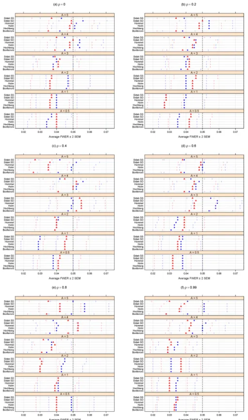
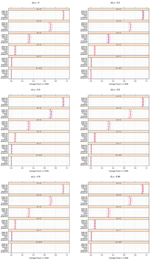
Figs1and2summarize the results of the simulation for the FWER-controlling methods. If the interest is to control the FWER, we note that all the FWER methods do indeed control the FWER equally well at the chosenαlevel (0.05 here), even in the presence of block-correlation positively-dependent tests, regardless of effect size (A), degree of dependence (ρ), or size of dependence group (Fig 1). As expected,Fig 2shows these methods’ power increases for larger magnitudes of differential abundance (i.e., larger effect sizesA). Power does not appear to be affected by increasing levels of dependence (i.e., largerρ) or dependence group size. Regardless of effect size (A) or degree of dependence (ρ), it appears best to use the Sidak SD, Hommel, Holm, or Hochberg methods, as there is a modest (but consistent) power loss in the Bonfer-roni and Sidak SS methods (Fig 2).
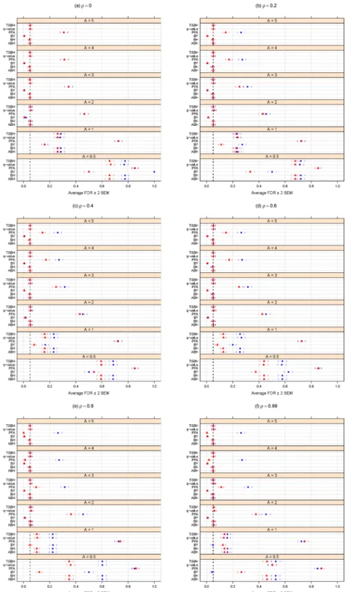
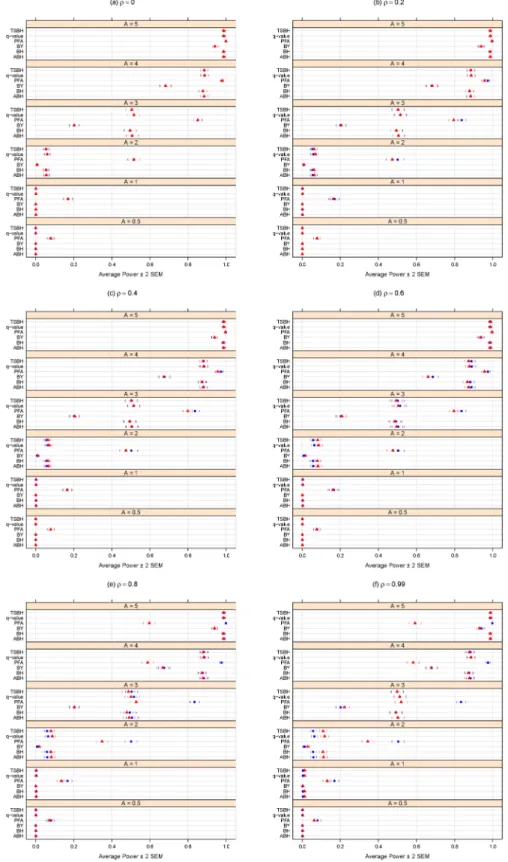
Figs3and4summarize simulation results for the FDR-controlling methods. FDR control (Fig 3) and statistical power (Fig 4) both improve, as expected, for larger magnitudes of differ-ential abundance (i.e., larger effect sizesA.)
Fig 3shows that increasing levels of dependence (i.e., largerρ) appears to improve FDR control for tests of small effects (such asA= 0.5), but has no clear effect for largerA.
Fig 3indicates that increasing the dependence group size (360 vs. 120) results in lower FDR when the effect is small (A= 0.5) andρis larger. Larger dependence group size also appears to result in a modest gain in (already poor) power (seeFig 4) among most FDR-controlling meth-ods when the effect is moderate (such asA= 2) andρis larger. However, for largerAand larger
ρ,Fig 4shows a possible (if negligible) loss of power.
Of the methods purporting to control the FDR, the PFA method generally has the best power (Fig 4), butFig 3shows that, at least for this large number of tests and for the block-cor-relation positively-dependent covariance structure shown inEq 1, the PFA method fails to pro-vide even reasonable control of the FDR. We note that this PFA performance includes the best-case scenario of treating the covariance matrix as known. Additional simulations described in Section B ofS1 Filesuggest that, at least for certain block-correlation positively-dependent covariance structures, the PFA method may provide better FDR control for smaller numbers of tests, but for larger numbers of tests (in the thousands), the PFA method does not provide the desired FDR control.
If the interest is to control the FDR, we note that, for at least moderate effect sizes (A2), the FDR methods (other than PFA) do indeed control the FDR at the chosenαlevel (0.05 here), regardless of the degree of dependence (ρ) (Fig 1). The Benjamini and Yekutieli proce-dure (BY) gives the most conservative control of the FDR (Fig 1), but at a noticeable loss of power (Fig 2). Regardless of effect size (A) or degree of dependence (ρ), it appears best to use the two stage Benjamini and Hochberg procedure (TSBH), the q-value method, or the adaptive Benjamini and Hochberg procedure (ABH) to control the FDR, even when positive block cor-relation dependence is present.
We conclude with a few caveats. First, the multiple hypothesis testing literature is evolving, so the above recommendations will not necessarily remain the best in perpetuity. Also, we only considered a certain class of dependence among test results, and any simulation study can
Fig 1. Average FWER for different methods purporting to control the FWER atα= 0.05. A can be
thought of as the magnitude of differential abundance for truly differentially abundant features, andρis the true correlation within blocks of dependent tests. The blue solid circles represent the case of 18 dependent tests (out of 100 total), whereas the red solid triangles are for the case of 36 dependent tests. Parentheses indicate±2 SEM.
Fig 2. Average power for different methods purporting to control the FWER atα= 0.05. A can be
thought of as the magnitude of differential abundance for truly differentially abundant features, andρis the true correlation within blocks of dependent tests. The blue solid circles represent the case of 18 dependent tests (out of 100 total), whereas the red solid triangles are for the case of 36 dependent tests. Parentheses indicate±2 SEM.
Fig 3. Average FDR for different methods purporting to control the FDR atα= 0.05. A can be thought of
as the magnitude of differential abundance for truly differentially abundant features, andρis the true correlation within blocks of dependent tests. The blue solid circles represent the case of 120 dependent tests (out of 2000 total), whereas the red solid triangles are for the case of 360 dependent tests. Parentheses indicate±2 SEM.
Fig 4. Average power for different methods purporting to control the FDR atα= 0.05. A can be thought
of as the magnitude of differential abundance for truly differentially abundant features, andρis the true correlation within blocks of dependent tests. The blue solid circles represent the case of 120 dependent tests (out of 2000 total), whereas the red solid triangles are for the case of 360 dependent tests. Parentheses indicate±2 SEM.
not reasonably consider all possible conditions (see the concluding two paragraphs of the “Methods: simulation analysis” Section above). Nevertheless, these results do provide a con-crete comparison of multiplicity adjustment methods and give some insight as to the effects of degree of differential feature abundance (A), degree of dependence among tests (ρ), and sizes of dependence groups on error rate control and power. In addition, this comparison and all the panels of Figs1–4are completely reproducible using the R code provided inS2 File.
Supporting information
S1 File. Background information on previous literature, including multiple testing adjust-ment methods and dependence among test results.
(PDF)
S2 File. R code to reproduce the entire simulation, including data analysis and summary figure panels.
(R)
Author Contributions
Conceptualization: JRS AAM. Data curation: JRS AAM. Formal analysis: JRS AAM AS. Funding acquisition: JRS. Investigation: JRS AAM. Methodology: JRS AAM. Project administration: JRS. Software: JRS AAM AS. Supervision: JRS. Validation: AS.
Visualization: JRS AAM.
Writing – original draft: JRS AAM. Writing – review & editing: JRS AAM AS.
References
1. Dudoit S, Shaffer JP, Boldrick JC. Multiple hypothesis testing in microarray experiments. Statistical Sci-ence. 2003; p. 71–103.https://doi.org/10.1214/ss/1056397487
2. Elliott P, Wartenberg D. Spatial epidemiology: current approaches and future challenges. Environmen-tal Health Perspectives. 2004; 112(9):998–1006.https://doi.org/10.1289/ehp.6735PMID:15198920 3. Bennett CM, Wolford GL, Miller MB. The principled control of false positives in neuroimaging. Social
Cognitive and Affective Neuroscience. 2009; 4(4):417–422.https://doi.org/10.1093/scan/nsp053PMID:
20042432
4. Lindquist MA, Meijia A. Zen and the art of multiple comparisons. Psychosomatic Medicine. 2015; 77(2): 114–125.https://doi.org/10.1097/PSY.0000000000000148PMID:25647751
5. Benjamini Y, Hochberg Y. Controlling the false discovery rate: a practical and powerful approach to mul-tiple testing. Journal of the Royal Statistical Society Series B (Methodological). 1995; p. 289–300.
6. Storey JD. A direct approach to false discovery rates. Journal of the Royal Statistical Society: Series B (Statistical Methodology). 2002; 64(3):479–498.https://doi.org/10.1111/1467-9868.00346
7. Benjamini Y, Yekutieli D. The control of the false discovery rate in multiple testing under dependency. Annals of Statistics. 2001; p. 1165–1188.
8. Fan J, Han X, Gu W. Estimating false discovery proportion under arbitrary covariance dependence. Journal of the American Statistical Association. 2012; 107(499):1019–1035.https://doi.org/10.1080/ 01621459.2012.720478PMID:24729644
9. Bonferroni CE. Teoria statistica delle classi e calcolo delle probabilita. Libreria Internazionale Seeber; 1936.
10. Sˇ ida´k Z. Rectangular confidence regions for the means of multivariate normal distributions. Journal of the American Statistical Association. 1967; 62(318):626–633.https://doi.org/10.1080/01621459.1967. 10482935
11. Holland BS, Copenhaver MD. An improved sequentially rejective Bonferroni test procedure. Biometrics. 1987; p. 417–423.https://doi.org/10.2307/2531823
12. Holm S. A simple sequentially rejective multiple test procedure. Scandinavian Journal of Statistics. 1979; p. 65–70.
13. Hommel G. A stagewise rejective multiple test procedure based on a modified Bonferroni test. Biome-trika. 1988; 75(2):383–386.https://doi.org/10.1093/biomet/75.2.383
14. Hochberg Y. A sharper Bonferroni procedure for multiple tests of significance. Biometrika. 1988; 75(4): 800–802.https://doi.org/10.1093/biomet/75.4.800
15. Sarkar SK. Some probability inequalities for ordered MTP2 random variables: a proof of the Simes con-jecture. Annals of Statistics. 1998; p. 494–504.
16. Benjamini Y, Hochberg Y. On the adaptive control of the false discovery rate in multiple testing with independent statistics. Journal of Educational and Behavioral Statistics. 2000; 25(1):60–83.https://doi. org/10.2307/1165312
17. Benjamini Y, Krieger AM, Yekutieli D. Adaptive linear step-up procedures that control the false discov-ery rate. Biometrika. 2006; 93(3):491–507.https://doi.org/10.1093/biomet/93.3.491
18. Nichols T, Hayasaka S. Controlling the familywise error rate in functional neuroimaging: a comparative review. Statistical Methods in Medical Research. 2003; 12:419–446.https://doi.org/10.1191/ 0962280203sm341raPMID:14599004
19. Suyundikov A, Stevens JR, Corcoran C, Herrick JS, Wolff RK, Slattery ML. Accounting for dependence induced by weighted KNN imputation in paired samples, motivated by a colorectal cancer study. PLOS ONE. 2015; 10(4):e0119876.https://doi.org/10.1371/journal.pone.0119876PMID:25849489 20. Suyundikov A, Stevens JR, Corcoran C, Herrick JS, Wolff RK, Slattery ML. Incorporation of
subject-level covariates in quantile normalization of miRNA data. BMC Genomics. 2015; 16:1045.https://doi. org/10.1186/s12864-015-2199-4PMID:26653287
21. Kohler JR, Guennel T, Marshall SL. Analytical strategies for discovery and replication of genetic effects in pharmacogenomic studies. Pharmacogenomics and Personalized Medicine. 2014; 7:217–225.
https://doi.org/10.2147/PGPM.S66841PMID:25206308
22. Morin A, Laviolette M, Pastinen T, Boulet LP, Laprise C. Combining omics data to identify genes associ-ated with allergic rhinitis. Clinical Epigenetics. 2017; 9(3).https://doi.org/10.1186/s13148-017-0310-1