Dynamic frequent itemset mining based on Matrix Appriori algorithm

(1)

DYNAMIC FREQUENT ITEMSET MINING BASED

ON MATRIX APRIORI ALGORITHM

A Thesis Submitted to

the Graduate School of Engineering and Sciences of

˙Izmir Institute of Technology

in Partial Fulfillment of the Requirements for the Degree of

MASTER OF SCIENCE

in Computer Engineering

by

Damla O ˘

GUZ

June 2012

˙IZM˙IR

(2)

We approve the thesis ofDamla O ˘GUZ

Examining Committee Members:

Assist. Prof. Dr. Belgin ERGENC¸

Department of Computer Engineering ˙Izmir Institute of Technology

Assist. Prof. Dr. Murat Osman ¨UNALIR

Department of Computer Engineering Ege University

Inst. Dr. Selma TEK˙IR

Department of Computer Engineering ˙Izmir Institute of Technology

25 June 2012

Assist. Prof. Dr. Belgin ERGENC¸

Supervisor, Department of Computer Engineering ˙Izmir Institute of Technology

Prof. Dr. ˙I. Sıtkı AYTAC¸ Prof. Dr. R. Tu˘grul SENGER

Head of the Department of Dean of the Graduate School of

(3)

ACKNOWLEDGMENTS

I would like to express my sincere gratitude to my thesis advisor,Assist. Prof. Dr. Belgin Ergenc¸, for her supervision and encouragement throughout the development of this thesis.

I would also like to thank my lecturers and colleagues in ˙Izmir Institute of Tech-nology Department of Computer Engineering. It has been a true pleasure to work in such a friendly environment. I am also grateful toBarıs¸ Yıldızfor his support in some of the important steps of this study as well.

I would like to state my special thanks to my dear husband Kaya O˘guz, for his endless support, patience, motivation and love. I would also like to thank my mother-in-lawS¸¨ukriyeand father-in-lawM. Cengiz O˘guzfor making contribution to our happy life with their understanding.

Finally, I would like to express my thanks to my motherAys¸enur, my fatherErkan

and my twin sisterDuygu Demirtas¸for supporting me throughout my whole life as well as in my graduate study. It is an immense blessing to have a family like them.

(4)

ABSTRACT

DYNAMIC FREQUENT ITEMSET MINING BASED ON MATRIX APRIORI ALGORITHM

The frequent itemset mining algorithms discover the frequent itemsets from a database. When the database is updated, the frequent itemsets should be updated as well. However, running the frequent itemset mining algorithms with every update is inefficent. This is called the dynamic update problem of frequent itemsets and the solution is to devise an algorithm that can dynamically mine the frequent itemsets.

In this study, a dynamic frequent itemset mining algorithm, which is called Dy-namic Matrix Apriori, is proposed and explained. In addition, the proposed algorithm is compared using two datasets with the base algorithm Matrix Apriori which should be re-run when the database is updated.

(5)

¨

OZET

“MATRIX APRIORI” ALGOR˙ITMASINI TEMEL ALAN DEV˙INGEN SIK K ¨UMELER MADENC˙IL˙I ˘G˙I

Sık kümeler madencili˘gi algoritmaları, sık kümeleri bir veritabanından ortaya çıkarırlar. E˘ger veritabanı güncellenirse, sık kümelerin de güncellenmesi gerekir. Fakat, her güncellemenin ardından algoritmaları bas¸tan çalıs¸tırmak verimsizdir. Bu probleme sık kümelerin devingen güncelleme problemi denir ve çözümü sık kümeleri devingen olarak bulabilecek bir algoritma ile mümkündür.

Bu çalıs¸mada, bir devingen sık kümeler madencili˘gi algoritması, Devingen Ma-trix Apriori, önerilmis¸ ve açıklanmıs¸tır. Buna ek olarak, önerilen algoritma, veritabanı güncellendi˘ginde yeniden çalıs¸tırılması gereken temel algoritma Matrix Apriori ile iki veriseti kullanılarak kars¸ılas¸tırılmıs¸tır.

(6)

LIST OF FIGURES

Figure Page

Figure 2.1. FP-tree Construction. . . 5

Figure 2.2. SOTrieIT Construction. . . 8

Figure 3.1. Matrix Apriori Example. . . 12

Figure 3.2. Dynamic Matrix Apriori - Before Increments. . . 14

Figure 3.3. Dynamic Matrix Apriori - After Additions. . . 15

Figure 3.4. Update Process in Dynamic Matrix Apriori for Additions. . . 15

Figure 3.5. Dynamic Matrix Apriori - After Deletions. . . 17

Figure 3.6. Update Process in Dynamic Matrix Apriori for Deletions. . . 17

Figure 4.1. Total Time with Different Addition Sizes on Dataset 1. . . 20

Figure 4.2. Speed-up with Different Addition Sizes on Dataset 1. . . 21

Figure 4.3. Total Time with Different Addition Sizes on Dataset 2. . . 22

Figure 4.4. Speed-up with Different Addition Sizes on Dataset 2. . . 22

Figure 4.5. Total Time with Different Deletion Sizes when Addition is 20% (Dataset 1). . . 25

Figure 4.6. Speed-up with Different Deletion Sizes when Addition is 20% (Dataset 1). . . 25

Figure 4.7. Total Time with Equal Addition and Deletion Sizes (Dataset 1.) . . . 27

Figure 4.8. Speed-up with Equal Addition and Deletion Sizes (Dataset 1). . . 27

Figure 4.9. Total Time with Different Deletion Sizes when Addition is 20% (Dataset 2). . . 29

Figure 4.10. Speed-up with Different Deletion Sizes when Addition Size is 20% (Dataset 2). . . 29

Figure 4.11. Total Time with Equal Addition and Deletion Sizes (Dataset 2). . . 31

(9)

LIST OF TABLES

Table Page

Table 2.1. Comparison of Incremental Itemset Mining Algorithms. . . 10

Table 4.1. Properties of Case 1 and Case 2. . . 23

Table 4.2. Comparison of Case 1 on Datase 1 and Dataset 2. . . 33

(10)

CHAPTER 1

INTRODUCTION

Association rule mining, which was introduced by Agrawal et al. (1993), has be-come a popular research area due to its applicability in various fields such as market analysis, forecasting and fraud detection. Given a market basket dataset, association rule mining discovers all association rules such as “A customer who buys itemX, also buys itemY at the same time”. These rules are displayed in the form ofX →Y whereX and

Y are sets of items that belong to a transactional database. Support of association rule

X → Y is the percentage of transactions in the database that contain X∪Y. Associa-tion rule mining aims to discover interesting relaAssocia-tionships and patterns among items in a database. It has two steps; finding all frequent itemsets and generating association rules from the itemsets discovered. Itemset denotes a set of items and frequent itemset refers to an itemset whose support value is more than the threshold described as the minimum support.

Since the second step of the association rule mining is straightforward, the gen-eral performance of an algorithm for mining association rules is determined by the first step (Han and Kamber (2006)). Therefore, association rule mining algorithms commonly concentrate on finding frequent itemsets. For this reason, in this thesis, “association rule mining algorithm” and “frequent itemset mining algorithm” terms are used interchange-ably.

Apriori and FP-Growth are known to be the two important algorithms each having different approaches in finding frequent itemsets (Agrawal and Srikant (1994) and Han et al. (2000)). The Apriori Algorithm uses Apriori Property in order to improve the effi-ciency of the level-wise generation of frequent itemsets. On the other hand, the drawbacks of the algorithm are candidate generation and multiple database scans. FP-Growth comes with an approach that creates signatures of transactions on a tree structure to eliminate the need of database scans and outperforms compared to Apriori (Han et al. (2000)). A recent algorithm called Matrix Apriori which combines the advantages of Apriori and FP-Growth was proposed (Pav´on et al. (2006)). The algorithm eliminates the need of multiple database scans by creating signatures of itemsets in the form of a matrix. The algorithm

(11)

provides a better overall performance than FP-Growth (Yildiz and Ergenc (2010)). Al-though all of these algorithms handle the problem of association rule mining, they ignore the dynamicity of the databases. When new transactions arrive or some transactions are deleted from the database, the problem of repeating the entire process from the beginning occurs. The solution to this problem is dynamic itemset mining in which the idea is to keep frequent itemsets up-to-date with arrival of increments to the database.

In this thesis, a new approach for dynamic frequent itemset mining based on Ma-trix Apriori Algorithm is proposed and compared with re-running MaMa-trix Apriori. The goal and the structure of the thesis are given in the following subsections.

1.1. Aim of the Thesis

Databases are updated continuously with additions and deletions in increments. When new transactions arrive to the database or some transactions are needed to be deleted from the database or they are added or deleted at once, the frequent itemset mining algorithms should be re-run in order to find up-to-date frequent itemsets. Since re-running the algorithms is time consuming, a dynamic frequent itemset mining algorithm, which is based on Matrix Apriori Algorithm, is proposed in the present study.

The objectives of this thesis are:

• To understand frequent itemset mining and dynamic frequent itemset mining. • To propose a dynamic frequent itemset mining algorithm.

• To compare the proposed dynamic frequent itemset mining algorithm with re-running the base frequent itemset mining algorithm.

• To observe the effects of additions for different databases. • To observe the effects of deletions for different databases.

(12)

1.2. Thesis Organization

The organization of this thesis is as follows:

• Chapter 2 “Related Work” gives general information about association rule mining and frequent itemset mining. Several important association rule mining algorithms are also presented and followed by a review of dynamic itemset mining algorithms.

• Chapter 3 proposes Dynamic Matrix Apriori Algorithm. First, the base algorithm Matrix Apriori is explained, and then the presentation of Dynamic Matrix Apriori is provided with two examples. The first example shows how the proposed algorithm handles additions and the second one demonstrates how deletions are handled.

• Chapter 4 shows the test results and the performance evaluations. The chapter be-gins with a presentation of the dataset properties. Then, this chapter is divided into two subsections. The test of the first subsection shows how the percentage of the addition sizes affects the performances of the Dynamic Matrix Apriori and the Ma-trix Apriori Algorithms. The test of the second subsection demonstrates how the percentage of the deletion sizes affects the performances of the algorithms. Two databases of different characteristics are used for evaluations.

• Chapter 5 is the conclusion chapter. A summary of the thesis and suggestions for future research are stated.

(13)

CHAPTER 2

RELATED WORK

Association rule mining aims to discover the relationships and the patterns in a dataset by including two steps: i) finding all frequent itemsets and ii) generating associ-ation rules from those frequent itemsets. The frequency of an itemset is also referred to as the support count, which is the number of transactions that contain the itemset. An itemset is named as frequent itemset if its support count satisfies the minimum support threshold (Han and Kamber (2006)). Minimum support and minimum support threshold are used interchangeably. Confidence, which assesses the strength of an association rule, is another measure for defining association rules. The confidence for an association rule

X →Y is the ratio of transactions that containX∪Y to the number of transactions that containX(Dunham (2002)). A formal definition of association rule mining is:

Given a set of itemsI={I1, I2,· · · , Im}and a database of transactionsD={T1, T2,

· · ·, Tn} where each transaction T is a set of items such thatT ⊆ I, and X, Y are set

of items, the association rule mining problem is to identify all association rulesX → Y with a minimum support and confidence, where support of association ruleX →Y is the percentage of transactions in the database that containX∪Y, and confidence is the ratio of support ofX∪Y to support ofX(Dunham (2002) and Han et al. (2000)).

2.1. Association Rule Mining Algorithms

The Apriori Algorithm is one of the best-known association rule mining algo-rithms (Wu et al. (2007)). It uses prior knowledge of frequent itemset properties and runs an iterative approach called level-wise search. That is, k−itemsets are used to ex-plore(k+ 1)−itemsets (they are called candidate itemsets before testing them against the database) by eliminating the candidates that do not satisfy the minimum support. This process terminates when no frequent or candidate set can be generated. The efficiency of the level-wise generation of frequent itemsets is improved by the Apriori Property: “All nonempty subsets of a frequent itemset must be frequent”. By means of this property, many unnecessary candidate generation and support counting are eliminated (Han and

(14)

Kamber (2006)). This property is used in many other association rule mining algorithms such as Fast Update Algorithm (Cheung et al. (1996)), Fast Update 2 Algorithm (Cheung et al. (1997)), FP-Growth Algorithm (Han et al. (2000)) and Matrix Apriori Algorithm (Pav´on et al. (2006)).

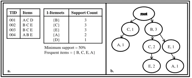
FP-Growth Algorithm handles the weaknesses of Apriori which are multiple scans of the database and candidate generation. It finds frequent itemsets without candidate generation by using a tree structure, called FP-tree, where each node stores an item with its number of occurrence in the database and a link to the next node. FP-tree creation is shown in Figure 2.1. First, frequent items are determined from the database as in Figure 2.1.a and then the tree is constructed as in Figure 2.1.b. A header table, in which frequent items with their support counts are kept in a descending order of support counts, is built to simplify tree traversal. The frequent itemsets are discovered with only two scans over the database. The first scan is for getting frequent 1-itemsets and their support counts same as the Apriori Algorithm and the second one is for generating the FP-tree. When the minimum support decreases, the length of frequent items and the number of candidate items increase consequently in Apriori. Therefore, FP-Growth performs better than Apriori when minimum support value is decreased (Han et al. (2000) and Zheng et al. (2001)). TID Items 001 002 003 004 A C D B C E B C E A B E

1-Itemsets Support Count

{B} {C} {E} {A} {D} 3 3 3 2 1 a. Minimum support = 50% Frequent items = { B, C, E, A} C, 1 A, 1 B, 3 C, 2 E, 1 E, 2 A, 1 b.

Figure 2.1. FP-tree Construction.

The Matrix Apriori Algorithm offers a simple and efficient solution to the as-sociation rule mining. Database scan step is similar to FP-Growth whereas generating association rules from discovered patterns is similar to Apriori. As a result, Matrix

(15)

Apri-ori combines the two algApri-orithms by using their positive properties (Pav´on et al. (2006)). Yildiz and Ergenc (2010) compared FP-Growth and Matrix Apriori algorithms by using different characteristics of data and found that the total performance of the Matrix Apriori is better than FP-Growth for minimum support values below 10%.

All of the algorithms above ignore the dynamicity of the databases. However, transactional databases are dynamic in general. When new transactions arrive or some transactions are deleted from the database, these algorithms should be re-run in order to find the current frequent itemsets. Dynamic frequent itemset mining is the solution for that problem.

2.2. Dynamic Association Rule Mining Algorithms

First group of incremental itemset mining algorithms are Apriori based (Cheung et al. (1997), Woon et al. (2001) and Amornchewin and Kreesuradej (2007)). Fast UP-date (FUP) Algorithm is the first algorithm proposed for incremental mining of frequent itemsets. It handles the databases with transaction insertion only and uses the pruning techniques used in Direct Hashing and Pruning Algorithm (Park et al. (1995)). The main working principle of this algorithm can be summarized in two steps. In the first step only new transactions are scanned to generate 1-itemsets. In the second step these itemsets are compared with the previous ones and all frequent itemsets of the same size are discovered iteratively. There are four possible cases in this algorithm when new transactions added:

• Case 1: If the itemset is frequent both in the original database and the new transac-tions, the itemset is always frequent.

• Case 2: If the itemset is frequent in the original database but infrequent in the new transactions, the frequency of the itemset is determined from the existing informa-tion.

• Case 3: If the itemset is infrequent in the original database but frequent in the new transactions, the original database should be scanned in order to determine frequent itemsets.

• Case 4: If the itemset is infrequent both in the original database and the new trans-actions, the itemset is always infrequent.

(16)

The original database should be scanned only in Case 3. In the first iteration, new transactions are scanned. If the itemset is frequent in the original database, the support count is calculated by adding the supports in the original database and the new transac-tions. This support count is compared with the support threshold of the updated database and if it does not satisfy the support threshold, the item is accepted as a loser and is pruned. Otherwise, when the itemset satisfies the support threshold, it remains to be fre-quent in the updated database. If the itemset is not frefre-quent in the original database, it is a potential candidate set. If its support count fails to satisfy the minimum support threshold in the new transactions, the item is pruned. Otherwise, original database is scanned in order to determine its frequency. FUP significantly reduces the number of candidate sets generated and is found to be 3 to 7 times faster than re-running Apriori for small support threshold. For larger support, FUP still outperforms (Cheung et al. (1996)).

FUP2 copes with both insertion and deletion of transactions, was proposed by (Cheung et al. (1997)). The algorithm is an extended version of FUP and it is equivalent to FUP in the insertion case. Previous mining results are used in order to find frequent itemsets in the insertion case and in the deletion case as well. The frequentk−itemsets from previous mining results are used in order to divide the candidate setCkintoPk and

QkwherePkis the set of candidate itemsets which have been frequent previously andQk

is the set of candidate itemsets, which have been infrequent before. The support counts of any candidate item inPkare known from previous mining result, so scanning only deleted

and inserted transactions is enough to update the support counts of candidates inPk. The

main working principle can be summarized in two steps. First, the deleted transactions are scanned so some candidate items can be deleted fromPk. On the other hand, the support

counts of itemsets inQkare unknown because they have been infrequent. However, when

an itemset inQkis frequent in the deletions, it must be infrequent in the updated database.

Second, the inserted transactions are scanned. The insertion case is the same as FUP. Although, FUP2 runs faster than Apriori, when the increment size is more than 40%, Apriori performs better (Woon et al. (2001)).

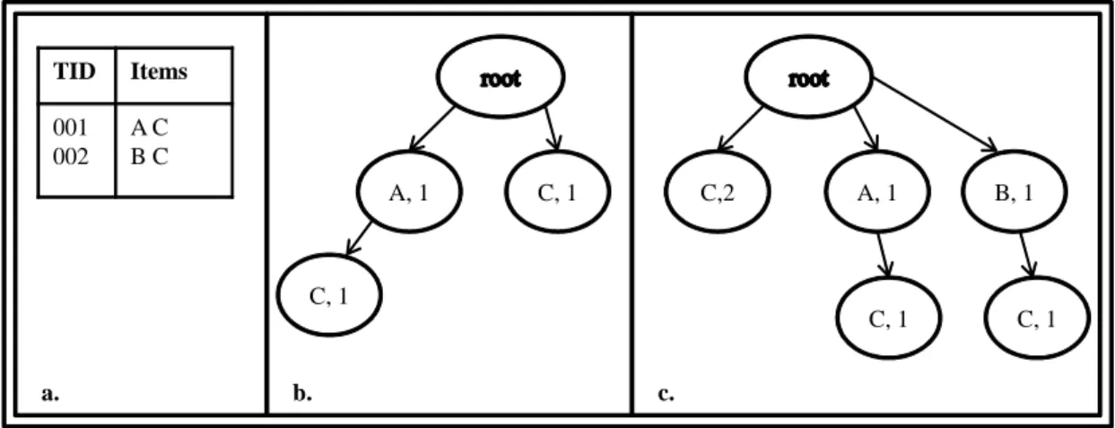
FOLDARM is another algorithm and was presented by Woon et al. (2001). It is suitable for dynamic association rule mining and it constructs a new data structure called Support-Ordered Trie Itemset, SOTrieIT (a trie-like tree structure). This structure only stores the frequent 1-itemsets and 2-itemsets with their supports in a descending order of support counts (the most frequent itemsets are found on the leftmost branches of the SOTrieIT) and is used to discover frequent 1-itemsets and 2-itemsets without scanning

(17)

the database. When new transactions arrive, all frequent 1-itemsets and 2-itemsets are extracted from each transaction. The extracted information is used to update the SOTrieIT without considering the support threshold. In order to mine frequent itemsets, depth-first search is used starting from the leftmost first-level node. Unless a node that does not satisfy the support threshold, the traversal continues. Subsequently, the Apriori Algorithm is used to obtain other frequent itemsets. Figure 2.2.b and Figure 2.2.c represents the SOTrieIT for the database in Figure 2.2.a (Woon et al. (2001)).

TID Items 001 002 A C B C A, 1 C, 1 C, 1 c. C,2 A, 1 B, 1 C, 1 a. b. C, 1

Figure 2.2. SOTrieIT Construction.

The study by Amornchewin and Kreesuradej (2007) proposed an incremental itemset mining algorithm based on Apriori. The presented algorithm finds frequent item-sets and infrequent itemitem-sets that are likely to be frequent after the arrival of new trans-actions. This algorithm uses the maximum support count of 1-itemsets in the database before the arrival of increments for finding potential frequent itemsets, called promising itemsets. In other words, in order to find a threshold value for finding promising itemsets, the maximum support count of 1-itemsets is used. It scans only new transactions, however it assumes that minimum support value does not change.

Second group of incremental itemset mining algorithms are focused on construct-ing the FP-tree incrementally (Hong et al. (2008) and Muhaimenul et al. (2008)). A fast updated FP-tree (FUFP-tree) structure and an incremental FUPF-tree maintenance algo-rithm was proposed by Hong et al. (2008). The links between nodes in FUFP-tree are bi-directional, which speeds up the process of item deletion. The four possible cases in FUP are the same in this algorithm. The header table and the tree are updated according to these cases. In the maintenance process of FUFP-tree, item deletion is done before the

(18)

item insertion. When a frequent item becomes infrequent after the increments, the item is deleted from the tree and its parent and child nodes are linked to each other. When an infrequent item becomes frequent after the update, the item is inserted to the leaf nodes of FUFP-tree and added to the header table. In this algorithm, it is assumed that when an infrequent item becomes frequent after the increments, its support value is usually a little bit more than the minimum support, so the updating process can be done as explained. However, when a sufficiently large number of transactions are inserted to the database, the whole FUFP-tree should be re-constructed (Hong et al. (2008)).

Muhaimenul et al. (2008) presented another method for constructing FP-tree in-crementally. The proposed algorithm avoids a full database scan when new transactions are added to the database. The minimum support threshold is accepted as 1 and FP-tree is updated by scanning the new transaction twice. Five synthetic and one real datasets are used in the experiments with different number of items and transactions. In both cases, this approach performs better compared to FP-Growth approach that builds the tree from the beginning.

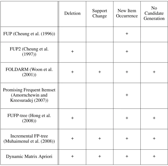
The comparison of incremental itemset mining algorithms is displayed in Table 2.1. All these algorithms can handle the maintenance problem in case of insertion and new items can be presented in the increments. FOLDARM, Incremental FP-tree and Dy-namic Matrix Apriori can handle minimum support change while FUP, FUP2, FUFP-tree and Promising Frequent Itemset cannot manage it. Also FUP, FUP2 and Promising Fre-quent Itemset need candidate generation. FOLDARM only addresses finding 1-freFre-quent itemsets and 2-frequent itemsets which is an important point to be taken into considera-tion.

(19)

Table 2.1. Comparison of Incremental Itemset Mining Algorithms. Deletion Support Change New Item Occurrence No Candidate Generation

FUP (Cheung et al. (1996)) +

FUP2 (Cheung et al.

(1997)) + +

FOLDARM (Woon et al.

(2001)) + + + +

Promising Frequent Itemset (Amornchewin and Kreesuradej (2007))

+

FUFP-tree (Hong et al.

(2008)) + + +

Incremental FP-tree

(Muhaimenul et al. (2008)) + + + +

(20)

CHAPTER 3

DYNAMIC MATRIX APRIORI ALGORITHM

Studies addressing dynamic update problem generally propose dynamic itemset mining methods based on Apriori and FP-Growth algorithms. Besides inheriting the dis-advantages of base algorithms, dynamic itemset mining has challenges as handling i) increments without re-running the algorithm, ii) support changes, iii) new items and iv) addition and deletions in increments.

Dynamic Matrix Apriori Algorithm is proposed to overcome the problem of min-ing frequent itemsets in dynamically updated databases. Oguz and Ergenc (2012) pro-vides a solution for increments composing of additions only. However, the core solution is extended to handle the deletion of transactions as well. As seen in Table 2.1, Dy-namic Matrix Apriori scans only new transactions in increments, handles new items in the additions, allows the change of support value and manages additions and deletions in increments.

This chapter is divided into two subsections where in the first the base algorithm Matrix Apriori, which works without candidate generation and scans database only twice, is explained to be self-contained. In the second subsection, Dynamic Matrix Apriori is presented.

3.1. Matrix Apriori Algorithm

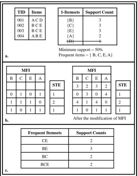
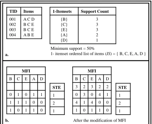
The Matrix Apriori Algorithm (Pav´on et al. (2006)) is a frequent itemset mining algorithm that combines the advantages of Apriori and FP-Growth algorithms. In this algorithm, the frequent items are stored in a matrix called MFI (Matrix of Frequent Items) and the supports of the patterns are stored in a vector called STE. Initially the database is scanned in order to determine frequent items. These items are sorted in a descending support count and trimmed to those that are above the minimum support value to create the frequent items list as in Figure 3.1.a. The sorted frequent items list is the basis for the order of columns of the MFI. Subsequently, in the second scan, MFI and STE are built as follows. The first row of the MFI is left empty. This row will be updated later in the

(21)

modification. Therefore, inserting rows to MFI begins after this empty row. For each new transaction in the database, a row of zeros and ones is inserted according to the following rule. The row is constructed by using the order in the frequent items list. For each item in the list, either “1” or “0” is added to the column of the row if the transaction contains the item or not. If the transaction is already included in the MFI, then it is not stored again in a new row, but its STE is incremented by “1”.

TID Items 001 002 003 004 A C D B C E B C E A B E

1-Itemsets Support Count

{B} {C} {E} {A} {D} 3 3 3 2 1 MFI B C E A 0 1 0 1 1 1 1 0 1 0 1 1 MFI B C E A 3 2 3 2 0 3 0 4 4 1 4 0 1 0 1 1 STE 1 2 1

After the modification of MFI

a. b. STE 1 2 1 Minimum support = 50% Frequent items = { B, C, E, A}

Frequent Itemsets Support Counts

CE 2

BE 3

BC 2

BCE 2

c.

Figure 3.1. Matrix Apriori Example.

After the construction of the matrix, it is modified in order to speed up the frequent itemset search. The first line of the MFI was left empty for this modification process. For each column, beginning from the first row, each cell value is set to the number of the row where the cell value is equal to “1” in the unmodified matrix. If there are not any

(22)

values of “1” in the remaining rows of the unmodified matrix, the cell value is set to “1”. Transactions can be reached from the individual frequent items through this reverse indexing. In Figure 3.1.b, the construction and modification of the matrix are shown. After the matrix construction, frequent itemsets are found as in 3.1.c. Beginning from the item that has the least support count; the item is compared with the items found on its left in order to find frequent itemsets. Following that, their support counts are calculated. The support count of an itemset is found by sequentially adding the related rows of STE from top to bottom.

Matrix Apriori works without candidate generation, scans database only twice and uses Apriori Property. Also, the management of matrix is easy.

3.2. Dynamic Matrix Apriori Algorithm

In order to provide dynamic mining of frequent itemsets, the matrix is constructed by the minimum support value of 1. That means all items are kept in the MFI without considering their frequencies. Doing so, flexibility for support change is enabled as well. Due to the structure of the matrix, items are kept in a descending support count in the MFI. So finding frequent itemsets with any support threshold is easy. Since all items are kept in the MFI, frequent itemsets can be calculated from the item that satisfies the minimum support when the support threshold is changed.

In this subsection, the proposed algorithm is explained and discussed with two examples. In the first example, only new transactions arrive to the database and in the second one, both additions and deletions appear in increments. The first example explains how Dynamic Matrix Apriori handles additions and the second example clarifies how the algorithm manages deletions of transactions.

The process before the arrival of increments for both additions and deletions are the same. The database is scanned and the support counts of items are calculated. All items are arranged in a descending order of support counts without considering if the item’s support count is more than the minimum support or not. The list of items in the specified order is named as 1-itemset ordered lists of items (IS). This process is depicted in Figure 3.2.a.

Afterwards, the MFI is constructed and then modified as in Figure 3.2.b. The method of construction and modification of the MFI and finding frequent itemsets are

(23)

TID Items 001 002 003 004 A C D B C E B C E A B E

1-Itemsets Support Count

{B} {C} {E} {A} {D} 3 3 3 2 1 MFI B C E A D 0 1 0 1 1 1 1 1 0 0 1 0 1 1 0 MFI B C E A D 3 2 3 2 2 0 3 0 4 1 4 1 4 0 0 1 0 1 1 0 STE 1 2 1

After the modification of MFI

a. b. STE 1 2 1 Minimum support = 50%

1- itemset ordered list of items (IS) = { B, C, E, A, D }

Figure 3.2. Dynamic Matrix Apriori - Before Increments.

the same as Matrix Apriori. When new transactions arrive or some transactions are to be deleted, the modified MFI is updated.

When new transactions arrive, they are scanned and 1-itemset ordered list of items are updated and named asISnew. This process is shown in Figure 3.3.a and indicated in

lines 1-2 of pseudo code in Figure 3.4. The new items in the additions are included to the MFI by adding new columns as in lines 3-5 in Figure 3.4. The MFI is updated as follows. First, the new transaction is checked whether it is existed in the MFI or not. If it exists, its STE is incremented by “1”; if it does not exist, it is added to the MFI. Adding to the MFI is done by setting the cell value to the row number of transaction where the “1” value is stored in the MFI. When the item does not exist in the remaining transactions of the incremental database, the cell value is set to “1”. This entire process is shown in Figure 3.3.b and in lines 6-12 in Figure 3.4. Finally, according to the change of the 1-itemset ordered list of items, the order of items in the MFI is changed as in Figure 3.3.c and in line of 13 in Figure 3.4.

(24)

TID Items

005 006

C D C F

1-Itemsets Support Count

{C} {B} {E} {A} {D} {F} 5 3 3 2 2 1 Minimum support = 50% IS_new= { C, B, E, A, D, F } MFI C B E A D F 2 3 3 2 2 6 3 0 0 4 5 0 5 4 4 0 0 0 0 1 1 1 0 0 6 0 0 0 1 0 1 0 0 0 0 1 a. b. MFI B C E A D F 3 2 3 2 2 6 0 3 0 4 5 0 4 5 4 0 0 0 1 0 1 1 0 0 0 6 0 0 1 0 0 1 0 0 0 1 STE 1 1 2 1 1 STE 1 1 2 1 1 c. MFI B C E A D 3 2 3 2 2 0 3 0 4 1 4 1 4 0 0 1 0 1 1 0 STE 1 2 1 Before additions Additions (A)

Figure 3.3. Dynamic Matrix Apriori - After Additions.

(25)

Figure 3.3 can be explained in detail as follows:

• When new transactions arrive to the database, additions are scanned and 1-itemset ordered list is updated (see Figure 3.3.a).

• A new column is included to the MFI for the new item, F.

• The MFI is searched whether the first transaction (C D) exists in the MFI or not. It does not exist in the MFI, so a new row is added to the MFI as the row number 5 and the MFI is updated as follows. Since the transaction containsCandD, the last MFI rows where these items have value “1” are found. ForC, this is row number 3 and the cell value “1” is updated as “5”. ForD, this is row number 2 and the cell value “1” is also updated as “5”. On row number 5 each item has value “1” for this transaction. For the following transaction, (C F), the procedure is repeated. This time value “1” ofCon the row number 5 is updated as “6” and on row 6, the cell value “1” is set. Fexists in this transaction for the first time. So the cell value of first row of F is set to “6” and the cell value of row number 6 is set to “1” (see Figure 3.3.a and Figure 3.3.b).

• The columns of the MFI are rearranged according to the 1-itemset ordered list of items (see Figure 3.3.c).

When some transactions are to be deleted, initially these transactions are scanned and 1-itemset ordered list of items are updated as in Figure 3.5.a and in lines 1-2 of pseudo code in Figure 3.6. This step is similar to the step when new additions arrive. Only difference of this step between additions and deletions is calculating the support counts of the items in the new transactions to be added or deleted. When new transactions arrive, the support counts of items in these transactions are incremented, however when some transactions are to be deleted, the support counts of items in these transactions are decreased (see Figure 3.5.a). Afterwards, the MFI is searched to find the row that will be deleted and its STE is decreased by “1” as seen in Figure 3.5.b and in lines 3-5 in Figure 3.6. Finally, according to the change of the 1-itemset ordered list of items, the order of items in the MFI is changed as in Figure 3.5.b and in line of 6 in Figure 3.6.

(26)

TID Items

001 002

A C D B C E

1-Itemsets Support Count

{B} {E} {A} {C} {D} 2 2 1 1 1 MFI B C E A D 3 2 3 2 2 0 3 0 4 1 4 1 4 0 0 1 0 1 1 0 a. b. STE 1 2 1 Minimum support = 50% IS_new= { B, E, A, C, D} MFI B E A C D 3 3 2 2 2 0 0 4 3 1 4 4 0 1 0 1 1 1 0 0 STE 0 1 1 Before deletions MFI B C E A D 3 2 3 2 2 0 3 0 4 1 4 1 4 0 0 1 0 1 1 0 STE 0 1 1 Deletions (D)

After column changes

Figure 3.5. Dynamic Matrix Apriori - After Deletions.

(27)

In brief, the Dynamic Matrix Apriori Algorithm provides a solution to the dynamic update problem. It handles both additions and deletions in increments and avoids a full database scan when the database is updated. Also, it avoids the construction of different matrices for mining frequent items with different support thresholds. Moreover, the base algorithm scans database only twice and does not generate candidate sets.

(28)

CHAPTER 4

PERFORMANCE EVALUATION

In this chapter, the Dynamic Matrix Apriori Algorithm is compared with the Ma-trix Apriori Algorithm when the database is updated. Since MaMa-trix Apriori does not have an update feature, it runs from the beginning on the updated database, while Dynamic Matrix Apriori only runs on the updates. Both algorithms are implemented in Java and test runs are performed on a computer with 2.93 GHz dual core processor and 2 GB mem-ory. During performance evaluations, it is ensured that the system state is similar in all test runs and they give similar results when they are repeated. Two synthetic datasets with different characteristics are used as in the performance evaluation of the work presented in Yildiz and Ergenc (2010). The synthetic datasets are generated by utilizing ARTool dataset generator by (Cristofor (2006)).

This chapter is divided into three subsections where in the first, two datasets are presented. In the second subsection, Dynamic Matrix Apriori is compared with re-running Matrix Apriori when new transactions are added to database. Finally, in the last one, these algorithms are analyzed when there are both additions and deletions in the increments.

4.1. Properties of Datasets

Dynamic Matrix Apriori and Matrix Apriori are tested against two datasets in order to see their performances on datasets having different characteristics.

The first dataset has the following characteristics i) long patterns and low diversity of items, ii) number of items is 10000, iii) average size of transactions is 20 and iv) average size of patterns is 10.

The second dataset is composed of the following characteristics i) short patterns and high diversity of items, ii) number of items is 30000, iii) average size of transactions is 20 and iv) average size of patterns is 5.

(29)

4.2. Performance with Additions

This subsection includes the performance analysis of the algorithms on two datasets while varying the size of new transactions. The purpose is to observe how the percentage of the addition sizes affects the performance of the algorithms for the generated datasets. The algorithms are compared for 20 increasing addition sizes in the range of 5% and 100%. In these tests, the minimum support is 10% and the initial database has 15000 transactions for both datasets.

4.2.1. Performance on Dataset 1

The performance of Matrix Apriori and Dynamic Matrix Apriori with different ad-dition sizes on Dataset 1 is demonstrated in Figure 4.1. In every increment size, Dynamic Matrix Apriori performs better than re-running Matrix Apriori.

0 100 200 300 400 500 600 0 20 40 60 80 100 T im e (s ec ) Addition size (%)

Matrix Apriori Dynamic Matrix Apriori

Figure 4.1. Total Time with Different Addition Sizes on Dataset 1.

In Figure 4.2, the speed-up with different addition sizes is illustrated. When the addition size is smaller, the speed-up is higher. The speed-up decreases from 92% to 45% as the addition size increases. Although the speed-up decreases as the addition size

(30)

increases, Dynamic Matrix Apriori is 45% faster than re-running Matrix Apriori with a 100% update.

The results on Dataset 1 indicate that Dynamic Matrix Apriori performs better than running Matrix Apriori with each addition update in the range between 5% and 100%.

0 20 40 60 80 100 0 20 40 60 80 100 S p ee d -u p ( % ) Addition size (%) Speed-Up

Figure 4.2. Speed-up with Different Addition Sizes on Dataset 1.

4.2.2. Performance on Dataset 2

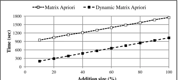
The results of Matrix Apriori and Dynamic Matrix Apriori with different addition sizes on Dataset 2 are shown in Figure 4.3. As expected, in every addition size, Dynamic Matrix Apriori performs better than the Matrix Apriori Algorithm similar to the results on Dataset 1.

As it is shown in Figure 4.4, the decrease in addition size increases the speed-up percentage from 41 to 81. Although there is a decrease in speed-up when the increment size becomes larger, Dynamic Matrix Apriori is almost 41% faster than re-running Matrix Apriori.

Both the test results on two datasets reveal that Dynamic Matrix Apriori performed better than running Matrix Apriori with each update in the range of 5% and 100%.

(31)

0 300 600 900 1200 1500 1800 0 20 40 60 80 100 T im e (s ec ) Addition size (%)

Figure 4.3. Total Time with Different Addition Sizes on Dataset 2.

0 20 40 60 80 100 0 20 40 60 80 100 S p ee d -u p ( % ) Addition size (%) Speed-Up

(32)

4.3. Performance with Additions and Deletions

The next comparison is to determine how the size of deletions affects the per-formances of algorithms. In these tests, there are both additions and deletions in the increments.

Performance analyses of the algorithms for the two different datasets with two cases are given in the following subsections. In Case 1, the number of added and deleted transactions varies independently. The initial database has 25000 transactions, then 5000 transactions are added to the database and the numbers of deleted transactions vary be-tween 1000 and 12000. In other words, in Case 1, the addition is constant (20% of the initial database) and the deletion percentage varies in the range of 4% to 48%. The pur-pose of the Case 1 is to observe how the percentage of the deletion sizes affects the performance of the algorithms for the generated datasets.

A test similar to Case 1 is done with the following properties. The initial database has 20000 transactions, then 10000 transactions are added to the database and the numbers of deleted transactions vary between 1000 and 10000. The addition size is constant again; however it is 50% of the initial database. That is, Dynamic Matrix Apriori is tested against the same purpose of Case 1 with different initial and addition sizes (see Appendix A for the test results).

In Case 2, the initial database has 20000 transactions and the number of added and the deleted transactions are the same. That is, n transactions are added to this database and othern transactions are deleted from it. The aim of it is to determine the effects of addition and deletion sizes. The properties of Case 1 and Case 2 are given in Table 4.1.

Table 4.1. Properties of Case 1 and Case 2.

Initial Database Size Addition Size Deletion Size

Case 1 25000 transactions 5000 transactions varies between 1000 to 12000

(33)

In these tests, it is assumed that entire update comes at once. So Matrix Apriori is run only once using a dataset that is the result of the additions and deletions. If these updates are done in different times, Matrix Apriori should have been run twice, while Dynamic Matrix Apriori should only run on the updates.

4.3.1. Performance on Dataset 1

Performance analyses of the Matrix Apriori and the Dynamic Matrix Apriori al-gorithms on Dataset 1 for Case 1 and Case 2 are given in this subsection.

Independently

The initial database consists of 25000 transactions. The database is updated with 5000 new transactions and varying size of deletions. Figure 4.5 illustrates the results of this test. As expected, Dynamic Matrix Apriori’s running time increases with the deletion size. On the other hand, Matrix Apriori’s running time decreases since the size of the updated database decreases. The results indicate that Dynamic Matrix Apriori performs better than re-running Matrix Apriori up to the deletion size of 44%.

The speed-up with different deletion sizes in this case is given in Figure 4.6. The speed-up decreases as does the number of deleted transactions. When the deletion amount is 4%, the speed-up is almost as high as 75%.

(34)

0 100 200 300 400 500 600 0 10 20 30 40 50 60 T im e (s ec ) Deletion size (%)

Figure 4.5. Total Time with Different Deletion Sizes when Addition is 20% (Dataset 1).

0 20 40 60 80 0 10 20 30 40 50 S p ee d -u p ( % ) Deletion size (%) Speed-Up

(35)

4.3.1.2. Case 2: Varying Number of Additions and Deletions Equally

In this case, the initial database has 20000 transactions. This database is updated with adding and deleting same amount of transactions. Figure 4.7 shows the comparison of Matrix Apriori and Dynamic Matrix Apriori. When the deletion size is more than 45%, re-running Matrix Apriori performs better. Dynamic Matrix Apriori’s running time increases as the update amount,n increases. On the other hand, running time of Matrix Apriori is not relevant to n. The reason of that is the size of the updated database is constant.

Figure 4.8 shows the speed-up when addition and deletion sizes are increased at every step but their sizes are kept the same. When the deletion size is 5%, the speed-up is almost 85%. However, the speed-speed-up decreases when the deletion size increases as expected.

(36)

0 100 200 300 400 0 10 20 30 40 50 T im e (s ec ) n (%)

Figure 4.7. Total Time with Equal Addition and Deletion Sizes (Dataset 1.)

0 20 40 60 80 100 0 10 20 30 40 50 S p ee d -u p ( % ) n (%) Speed-Up

(37)

4.3.2. Performance on Dataset 2

Performance analyses of the Matrix Apriori and the Dynamic Matrix Apriori al-gorithms on Dataset 2 for Case 1 and Case 2 are given in this subsection.

Independently

In these tests, the initial dataset has 25000 transactions and there are 5000 transac-tions of addition and varied size of deletransac-tions in the increments. The test results of running Dynamic Matrix Apriori and Matrix Apriori in these conditions are given in Figure 4.9. As foreseen, the running time of Dynamic Matrix Apriori increases as the the deletion size increases. On the other hand, the running time of Matrix Apriori decreases since the size of the updated database decreases. These results reveal that Dynamic Matrix Apriori is more efficient than Matrix Apriori until the size of deletions reaches 40%.

The speed-up with different deletion sizes in this case is shown in Figure 4.10. By the increasing number of the deleted transactions, the speed-up decreases. When the deletion amount is 4%, the speed-up is almost 66%.

(38)

0 300 600 900 1200 1500 1800 0 10 20 30 40 50 T im e (s ec ) Deletion size (%)

Figure 4.9. Total Time with Different Deletion Sizes when Addition is 20% (Dataset 2).

0 20 40 60 80 0 10 20 30 40 50 S p ee d -u p ( % ) Deletion size (%) Speed-Up

Figure 4.10. Speed-up with Different Deletion Sizes when Addition Size is 20% (Dataset 2).

(39)

4.3.2.2. Case 2: Varying Number of Additions and Deletions Equally

In this case, an initial database of 20000 transactions is used. This database is updated with the same size of additions and deletions. When the deletion size is more than 40%, Matrix Apriori performs better as seen in Figure 4.11. As expected, Dynamic Matrix Apriori’s running time increases as the update amount,n increases. On the other hand, since the size of the updated database is constant, running time of Matrix Apriori is not bound ton.

Figure 4.12 shows the speed-up with different deletion sizes when the numbers of transactions of addition and deletion sizes are the same. When the deletion size is 5%, the speed-up is almost 73%. However, the speed-up decreases when the deletion size increases.

(40)

0 300 600 900 1200 1500 0 10 20 30 40 50 T im e (s ec ) n (%)

Figure 4.11. Total Time with Equal Addition and Deletion Sizes (Dataset 2).

0 20 40 60 80 0 10 20 30 40 50 S p ee d -u p ( % ) n (%) Speed-Up

(41)

4.3.3. Discussion on Results

The tests in this subsection focus on the effects of deletion sizes in the increments. These effects are researched on two cases by using two different datasets. In Case 1 the addition size is constant (20%) and the deletion size is varied. The results of Case 1 in Dataset 1 and Dataset 2 is shown in Table 4.2. The speed-up can be observed up until the deletion size reaches 44% on Dataset 1. On Dataset 2, the speed-up exists up to until the deletion size is 40%. In addition, the speed-up is 19% on Dataset 1 when the deletion size is 40% (see Figure 4.6).

The deletions do not require significant changes in the MFI. Dynamic Matrix Apriori handles them by only decreasing their STE values and support count of items in deletions. This condition is reflected on to the results. In addition, with larger deletions Matrix Apriori handles a smaller dataset and this causes the speed-up ratio to go down as the number of deletions increase.

In Case 2, the initial database has 20000 transactions and the database is updated with n number of additions and other n number of deletions. The results of Case 2 in Dataset 1 and Dataset 2 is shown in Table 4.3. It should also be noted that as the value ofn increases, the database significantly changes. While this has little effect on Matrix Apriori since it runs from the beginning, Dynamic Matrix Apriori works on the same database with still better results.

(42)

Table 4.2. Comparison of Case 1 on Datase 1 and Dataset 2. Minimum Deletion Size Maximum Deletion Size Minimum Speed-up Maximum Speed-up Case 1 on Dataset 1 4% 44% 9% 75% Case 1 on Dataset 2 4% 40% 7% 66%

Table 4.3. Comparison of Case 2 on Datase 1 and Dataset 2.

Minimum Deletion Size Maximum Deletion Size Minimum Speed-up Maximum Speed-up Case 2 on Dataset 1 5% 45% 3% 85% Case 2 on Dataset 2 5% 40% 3% 73%

(43)

CHAPTER 5

CONCLUSION

Association rule mining aims to discover interesting patterns in a database. There are two steps in this data mining technique. The first step is finding all frequent itemsets and the second step is generating association rules from these frequent itemsets. Associa-tion rule mining algorithms generally focus on the first step since the second one is direct to implement. Although there are a variety of frequent itemset mining algorithms, they should be re-run when the database is updated in order to discover the up-to-date frequent itemsets.

This is time consuming and it should be repeated with every single update. There-fore, dynamic update problem of frequent itemsets occurs. The solution to this problem is dynamic frequent itemset mining.

In this study, a dynamic frequent itemset mining algorithm, called Dynamic Ma-trix Apriori is proposed. It is based on the MaMa-trix Apriori Algorithm. Dynamic MaMa-trix Apriori handles additions and deletions as well. It also manages the challenges of new items and support changes. The main advantage of the algorithm is avoiding the entire database scan when it is updated. It scans only the increments. The algorithm is com-pared with Matrix Apriori as follows. When the updates arrive, Matrix Apriori runs on the up-to-date database whereas Dynamic Matrix Apriori runs only with the updates.

The first part of this thesis is focused on the solution of additional update problem. Base algorithm Matrix Apriori works without candidate generation and scans database only twice bringing additional advantages. Performance studies show that Dynamic Ma-trix Apriori provides speed-up between 41% and 92% while increment size is varied be-tween 5% and 100%.

In the second study of this thesis, the Dynamic Matrix Apriori Algorithm is ex-tended as to handle the deletion of transactions as well. Comparison of the proposed al-gorithm and re-running Matrix Apriori revealed that Dynamic Matrix Apriori Alal-gorithm provides speed-up 7% to and 75% when the addition size is 20% and the deletion size is varied between 4% and 44%. It also provides speed-up 3% to and 85% when the addition and deletion size is varied between 5% and 45%.

(44)

Dynamic Matrix Apriori is dependent on the number of items in the dataset. As the number of items increase, the proposed algorithm would be handling more items since minimum support is always 1. As the diversity of the dataset increases Matrix Apriori has more advantage because the item count values would be lower and fewer numbers of items would be over the minimum threshold. However, up to almost 45% updates, Dynamic Matrix Apriori still performs better than a complete re-run. With only additions, Dynamic Matrix Apriori gives 45% better performance when the database is doubled.

For the upcoming studies, it is planned to compare the proposed approach with other incremental itemset mining algorithms in order to better understand its strengths and weaknesses. It is also scheduled to run the algorithm on real datasets. In addition, the algorithms should be tested with different minimum support values. It is expected that Dynamic Matrix Apriori will perform better when the support threshold decreases, since more items will be frequent for Matrix Apriori.

(45)

REFERENCES

Agrawal, R., T. Imieli´nski, and A. Swami (1993). Mining association rules between sets of items in large databases. InProceedings of the 1993 ACM SIGMOD International Conference on Management of Data, SIGMOD ’93, New York, NY, USA, pp. 207– 216. ACM.

Agrawal, R. and R. Srikant (1994). Fast algorithms for mining association rules in large databases. InProceedings of the 20th International Conference on Very Large Data Bases, VLDB ’94, San Francisco, CA, USA, pp. 487–499. Morgan Kaufmann Pub-lishers Inc.

Amornchewin, R. and W. Kreesuradej (2007, dec.). Incremental association rule mining using promising frequent itemset algorithm. InInformation, Communications Signal Processing, 2007 6th International Conference on, pp. 1 –5.

Cheung, D., J. Han, V. Ng, and C. Wong (1996, feb-1 mar). Maintenance of discov-ered association rules in large databases: An incremental updating technique. InData Engineering, 1996. Proceedings of the Twelfth International Conference on, pp. 106 –114.

Cheung, D. W.-L., S. D. Lee, and B. Kao (1997). A general incremental technique for maintaining discovered association rules. In Proceedings of the Fifth International Conference on Database Systems for Advanced Applications (DASFAA), pp. 185–194. World Scientific Press.

Cristofor, L. (2006). Artool project. http://www.cs.umb.edu/˜laur/ARtool/, Accessed: 30/06/2012.

Dunham, M. H. (2002).Data Mining: Introductory and Advanced Topics. Upper Saddle River, NJ, USA: Prentice Hall PTR.

Han, J. and M. Kamber (2006). Data Mining. Concepts and Techniques (2nd ed. ed.). Morgan Kaufmann.

(46)

Han, J., J. Pei, and Y. Yin (2000). Mining frequent patterns without candidate generation. InProceedings of the 2000 ACM SIGMOD International Conference on Management of Data, SIGMOD ’00, New York, NY, USA, pp. 1–12. ACM.

Hong, T.-P., C.-W. Lin, and Y.-L. Wu (2008). Incrementally fast updated frequent pattern trees.Expert Syst. Appl. 34(4), 2424–2435.

Muhaimenul, R. Alhajj, and K. Barker (2008). Alternative method for incrementally con-structing the fp-tree. In P. Chountas, I. Petrounias, and J. Kacprzyk (Eds.),Intelligent Techniques and Tools for Novel System Architectures, Volume 109 ofStudies in Com-putational Intelligence, pp. 361–377. Springer Berlin Heidelberg.

Oguz, D. and B. Ergenc (2012). Incremental itemset mining based on matrix apriori al-gorithm. In14th International Conference, DaWaK 2012. Springer. Accepted.

Park, J. S., M.-S. Chen, and P. S. Yu (1995). An effective hash-based algorithm for mining association rules. InProceedings of the 1995 ACM SIGMOD International Confer-ence on Management of Data, SIGMOD ’95, New York, NY, USA, pp. 175–186. ACM.

Pav´on, J., S. Viana, and S. G´omez (2006). Matrix apriori: Speeding up the search for frequent patterns. In Proceedings of the 24th IASTED International Conference on Database and Applications, DBA’06, Anaheim, CA, USA, pp. 75–82. ACTA Press.

Woon, Y.-K., W.-K. Ng, and A. Das (2001). Fast online dynamic association rule mining. InProceedings of the Second International Conference on Web Information Systems Engineering (WISE’01) Volume 1 - Volume 1, WISE ’01, Washington, DC, USA, pp. 278–. IEEE Computer Society.

Wu, X., V. Kumar, J. Ross Quinlan, J. Ghosh, Q. Yang, H. Motoda, G. J. McLachlan, A. Ng, B. Liu, P. S. Yu, Z.-H. Zhou, M. Steinbach, D. J. Hand, and D. Steinberg (2007, December). Top 10 algorithms in data mining.Knowl. Inf. Syst. 14(1), 1–37.

Yildiz, B. and B. Ergenc (2010). Comparison of two association rule mining algorithms without candidate generation. InProceedings of the 10th IASTED International

(47)

Con-ference on Artificial Intelligence and Applications, SIGMOD ’93, pp. 450–457. ACM.

Zheng, Z., R. Kohavi, and L. Mason (2001). Real world performance of association rule algorithms. In Proceedings of the Seventh ACM SIGKDD International Conference on Knowledge Discovery and Data Mining, KDD ’01, New York, NY, USA, pp. 401– 406. ACM.

(48)

APPENDIX A

MORE TEST RESULTS

The tests in Appendix A, called Case A, are executed on the same datasets in this thesis. The initial database has 20000 transactions. The database is then updated with 10000 additions (50% of the initial database) and different size of deletions.

Figure A.1 shows the test results of Case A on a dataset based on Dataset 1. Dy-namic Matrix Apriori performs better than Matrix Apriori up to the deletion size of 45%. The speed-up with different deletion sizes in Case A on a dataset based on Dataset 1 is given in Figure A.2. When the deletion amount is 5%, the speed-up is almost as high as 57%.

Figure A.3 demonstrates the test results of Case A on Dataset 2. They reveal that Dynamic Matrix Apriori is more efficient than Matrix Apriori until the size of deletions reach 40%.

The speed-up with different deletion sizes in Case A is shown in Figure A.4. By the increasing number of the deleted transactions, the speed-up decreases. When the deletion amount is 5%, the speed-up is almost 50%.

(49)

0 100 200 300 400 500 600 0 10 20 30 40 50 T im e (s ec ) Deletion size (%)

Figure A.1. Run-time with Different Deletion Sizes when Addition is 50% (Dataset 1).

0 10 20 30 40 50 60 0 10 20 30 40 50 S p ee d -u p ( % ) Deletion size (%) Speed-Up

(50)