White Rose Research Online URL for this paper:
http://eprints.whiterose.ac.uk/163748/
Version: Accepted Version
Article:
Zhou, L., Zhang, X., Wang, J. et al. (5 more authors) (2020) Subspace Structure
Regularized Nonnegative Matrix Factorization for Hyperspectral Unmixing. IEEE Journal of
Selected Topics in Applied Earth Observations and Remote Sensing. ISSN 2151-1535
https://doi.org/10.1109/JSTARS.2020.3011257
[email protected] https://eprints.whiterose.ac.uk/ Reuse
Items deposited in White Rose Research Online are protected by copyright, with all rights reserved unless indicated otherwise. They may be downloaded and/or printed for private study, or other acts as permitted by national copyright laws. The publisher or other rights holders may allow further reproduction and re-use of the full text version. This is indicated by the licence information on the White Rose Research Online record for the item.
Takedown
If you consider content in White Rose Research Online to be in breach of UK law, please notify us by
Subspace Structure Regularized Nonnegative Matrix
Factorization for Hyperspectral Unmixing
Lei Zhou, Xueni Zhang, Jianbo Wang, Xiao Bai, Lei Tong, Liang Zhang, Jun Zhou, and Edwin Hancock
Abstract—Hyperspectral unmixing is a crucial task for hy-perspectral images (HSI) processing, which estimates the pro-portions of constituent materials of a mixed pixel. Usually, the mixed pixels can be approximated using a linear mixing model. Since each material only occurs in a few pixels in real HSI, sparse nonnegative matrix factorization (NMF) and its extensions are widely used as solutions. Some recent works assume that materials are distributed in certain structures, which can be added as constraints to sparse NMF model. However, they only consider the spatial distribution within a local neighborhood and define the distribution structure manually, while ignoring the real distribution of materials that is diverse in different images. In this paper, we propose a new unmixing method that learns a subspace structure from the original image and incorporate it into the sparse NMF framework to promote unmixing performance. Based on the self-representation property of data points lying in the same subspace, the learned subspace structure can indicate the global similar graph of pixels that represents the real distribution of materials. Then the similar graph is used as a robust global spatial prior which is expected to be maintained in the decomposed abundance matrix. The experiments conducted on both simulated and real-world HSI datasets demonstrate the superior performance of our proposed method.
Index Terms—Hyperspectral unmixing, linear mixing model (LMM), nonnegative matrix factorization (NMF), subspace struc-ture, similar graph.
I. INTRODUCTION
H
YPERSPECTRAL image (HSI) analysis [1]–[5] is one of the fastest-growing technologies in recent years. However, due to low spatial resolution or specific imaging mechanism, the acquired hyperspectral images often contain This work was supported by NSFC No. 61772057, Beijing Natural Science Foundation(4202039) and the support funding from State Key Lab. of Soft-ware Development Environment and Jiangxi Research Institute of Beihang University.L. Zhou, X. Zhang, X. Bai and L. Zhang are with School of Computer Sci-ence and Engineering, Beijing Advanced Innovation Center for Big Data and Brain Computing, State Key Laboratory of Software Development Environ-ment, Jiangxi Research Institute, Beihang University, Beijing 100191, China. (e-mail:[email protected], [email protected], [email protected]).
J. Wang is with the First Clinical Medical College of Nanchang University, No. 461 Bayi Avenue, Nanchang, Jiangxi 330006, China ([email protected]).
L. Tong is with the Faculty of Information Technology, Beijing University of Technology, Beijing 100124, China (e-mail: lei [email protected]).
J. Zhou is with the School of Information and Communication Technology, Griffith University, Nathan, Qld. 4111, Australia (e-mail: [email protected]).
E. Hancock is with the Department of Computer Science, University of York, York, U.K. (e-mail: [email protected]).
The code for this paper is available on https://github.com/zlbuaa/Subspace-Regularized-Unmixing.
Lei Zhou, Xueni Zhang and Jianbo Wang are the co-first author. Xiao Bai and Liang Zhang are the corresponding author.
mixed pixels which span surface areas containing several types of materials. To effectively exploit hyperspectral data, hyperspectral unmixing (HU) [6]–[9] has become an basic preprocessing for effective HSI analysis.
The objective of hyperspectral unmixing is to decompose mixed pixels into components with the reference spectral signatures of each of the materials present (endmembers), and to determine their corresponding fractions (abundances). Ex-isting unmixing algorithms mainly exploit one of two mixture models, namely a) a linear model or b) a nonlinear model. Nonlinear mixing models [10], [11] assume that the observed pixel is mixed by a nonlinear function of the component spectral signatures of the endmembers which are weighted by the corresponding abundances. However, the process of nonlinear combination is usually difficult to model physically and to recover in real world applications. In recent years, linear mixing model (LMM) [12] has therefore been more widely adopted in most works on hyperspectral unmixing. The reason for this is the balance between model accuracy and tractability. LMM is based on the assumption that different endmembers are mutually independent, so that the observed HSI is a linear combination of the endmembers and their corresponding abundances.
Abundant LMM unmixing algorithms have been proposed. Some of these focus on the endmember extraction from statis-tical and geometrical aspects, such as Pixel Purity Index [13], N-FINDR [14], alternating projected subgradients [15], Ver-tex Component Analysis [16], independent component anal-ysis [17], and minimum-volume-based unmixing algorithm-s [18], etc. Other methodalgorithm-s addrealgorithm-salgorithm-s the problem of abundance estimation under the assumption that the endmembers are available [19]. With the almost universal success of deep learning, there are also examples of deep neural network based hyperspectral unmixing methods [20]–[22]. However, these methods depend on the availability of large amount of training data with groundtruth. In this paper, we focus on blind unmixing which learns the endmembers as well as their abundances simultaneously. Nonnegative Matrix Factorization (NMF) [23], [24] is the most commonly used method for blind source separation. It aims to decompose mixed data through the product of two nonnegative matrices. This is done by minimizing the reconstruction error as measured by Euclidean distance. However, the solution of NMF is usually not unique if there are no further constraints [25]. To alleviate this problem, two kinds of constraints are commonly used on the abundance matrix.
The first is the sparsity constraint for abundance matrix. This is based on the fact that the pixels of HSI are mostly
mixed by a relatively small number of endmembers. Therefore, [26], [27] presented a spare coding method on the abundance matrix for hyperspectral unmixing. In this paper, Lp denotes the p norm. In fact, provided Lp(0 ≤ p ≤ 1) then the regularizer has the effect of leading to a sparse solution. Moreover, the sparsity of the Lp(12 ≤ p ≤ 1) solution is
negatively correlated with p, but the sparsity of the solution for Lp(0 ≤ p ≤ 12) is not sensitive with the change of p. Therefore, Qian et al. [28] utilized the L1/2 regularizer
on the abundance matrix to constrain the sparseness. It has been proved that the L1/2 regularizer is more efficient in
computation compared to theL1 regularizer, and the solution
is also closer to the groundtruth. In addition, to avoid the influence of noise, many norm-based robust NMF methods have been proposed. The L2,1 norm is commonly integrated
into sparse NMF to achieve robustness for pixel noise and outlier rejection since it is rotationally invariant [19], [29], [30]. Additionally, theL1,2 norm is also effective for solving
band noise problems [31], [32].
The second type of contraint incorporates information con-cerning the spatial distribution into abundance estimation, and has proved useful in improving the unmixing results. This is due to the fact that endmembers are distributed to form co-herent geometric structures, and two correlated pixels usually have similar fractional abundances for the same endmembers. Therefore, the total variation (TV) regularizer [33]–[35] was incorporated to promote piece-wise smooth transitions in the abundance matrix for neighboring pixels of the same endmem-ber category. In [36], abundance separation and smoothness constrained NMF (ASSNMF) was proposed for hyperspectral unmixing. The abundance separation acted on the spectral domain, and the abundance smoothness constraint was used on the spatial domains to exploit the spatial information. Due to the spatial structure learning ability of manifold method, [37] incorporated manifold structures learning into the NMF model to separate similar neighboring pixels. Inspired by the denois-ing method [38], Lu et al. proposed a structure constrained sparse NMF (CSNMF) method [39] which exploited clustering based approach to find the potential structure information. In [40], a clustered multitask network was proposed to solve the unmixing problem, which also used the clustering method to explore the distribution. Recently, spatial group sparsity regularized NMF (SGSNMF) [41] utilized superpixels that are obtained from image segmentation as a spatial prior to promote hyperspectral unmixing.
Although the above methods try to exploit the spatial dis-tribution of pixels, all these methods explore the correlations of pixels within a local neighborhood, and most of them are defined manually. However, each material usually occurs in many different regions in the same hyperspectral image. Thus the spatial distribution of a particular material is not limited to local structures. Moreover, it is obvious that the distributions of materials may be quite diverse in different images. According to [42], each kind of land-cover material in a remotely sensed hyperspectral image can be treated as a different subspace. Although they might have different spectra because of the varying illumination, topography, and other imaging conditions. Therefore, the spatial distribution
infor-mation can be captured by the subspace structure [43]. This not only represents the global distribution of the materials but can also be learned from the corresponding image. Motivated by this fact, we propose a new method aimed at incorporating the subspace structure regularization into the sparse NMF-based unmixing process. In contrast to deep subspace learning method [44], [45], here we utilize a Low-Rank Represen-tation (LRR) method [46], [47] to learn the similar graph that represents the subspace structures for all materials and which contains the correlations of all pixel pairs. Since the LRR constraint can be incorporated into the NMF constraint, this offers the advantage that we can optimize the subspace learning and the hyperspectral unmixing simultaneously. As a result the spatial prior is integrated through regularization into sparse NMF and can be used to perform the hyperspectral unmixing. Furthermore, based on the assumption that an abundance matrix can be seen as the denoised feature vectors of the original image, the learned abundance matrix can be used to better learn the latent subspace structure. Hence, we introduce a novel joint framework to simultaneously optimize hyperspectral unmixing and subspace structure learning in a manner which leads to mutual enhancement.
The main contributions of this paper are summarized as follows:
1) We propose a new hyperspectral unmixing method which learns the subspace structure of material re-flectance to capture the global correlation of all pixels. Then the global similar graph for materials is used as a robust spatial prior to improve the quality of the hyperspectral unmixing.
2) We design an objective function to integrate the spectral-spatial based unmixing and subspace structure learning into a single unified framework, in which they can be jointly optimized by an iterative algorithm. The joint framework can not only enhance the unmixing performance but also provide better subspace clustering results.
3) Experiments on both simulated and real-world HSI datasets indicate the superiority of the proposed method, which achieves comparable performance to state-of-the-art methods for hyperspectral unmixing.
The remainder of this paper is structured as follows. Section II describes the background of the LMM and NMF algorithms. Section III presents our proposed method and demonstrates the implementation details. The experimental results on simulated data and real-world HSI data are presented in Section IV. Finally, we conclude this paper in Section V.
II. BACKGROUND
A. NMF for Hyperspectral Unmixing
The classic LMM for hyperspectral unmixing is based on the assumption that the observed HSI is a linear mixture of several endmembers. Consider a HSIY ∈RL×N
, where the number of wavelength-indexed bands isLand the number of pixels isN. Then the original dataYcan be reconstructed by a linear combination of endmembers as follow:
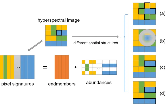
Fig. 1. Illustration of the concept of our method and several alternative methods. The original images are decomposed into two matrices: the endmembers matrix and the abundance matrix. When maintaining the spatial structure for each pixel in the abundance matrix, different methods utilized different strategies. Take the blue pixel marked with black box in the original image as an example, (a) TV regularizer considers its four neighborhood as the local structure; (b) manifold regularizer uses heat kernel to capture the local structure; (c) segmentation-based regularizer learns a local neighborhood; (d) our proposed method learns a subspace structure that represents the global distribution of each material.
where a)A∈RL×P
denotes the endmember matrix, in which each column represents the spectral signature of the corre-sponding endmember and P is the number of endmembers, b) S∈RP×N
denotes the abundance matrix, in which each column is the fractions of all endmembers in the corresponding pixel and c) E is an additive Gaussian white noise.
Since the goal of hyperspectral unmixing is to estimate the endmember and abundance matrices simultaneously, in this task, we only know the matrix Y, and matrices A and
S are the unknown targets of unmixing. To avoid the large solution space, two commonly adopted constraints can be used on the matrices A and S [48]. The first is the so-called abundance sum-to-one constraint, which restrict the proportions of each endmember sum to one. Another is the nonnegativity constraint, which restrict elements in both the endmember and abundance matrices must be greater than or equal to zero.
With the nonnegativity constraint, NMF is a good way to decompose the original image into the endmember and abun-dance matrices simultaneously. By reconstructing the original imageYthrough endmember matrixAand abundance matrix
S, the target of optimization can be defined as:
C(A,S) = 1
2kY−ASk 2
F s.t.A>0,S>0 (2) wherek·kF represents the Frobenius norm.
The multiplied iterative algorithm is commonly used to solve this objective function. When applied to Equation (2),
the multiplicative rule leads to the following two interleaved equations:
A=A.∗YST./ASST (3)
S=S.∗ATY./ATAS (4) where (·)T denotes the matrix transposition, .∗ denotes element-wise multiplication and./denotes element-wise divi-sion.
B. NMF with Sparsity Constraints
There are several drawbacks of the traditional NMF model (2). Firstly, it is nonconvex, which means it is hard to get the globally optimal solution. Secondly, the solution of this objective function is not unique, this is because AS can be replaced by (AD)(D−1S)
for any nonnegative invertible matrix D. Therefore, the classical NMF model will make the unmixing process unstable. To solve this problem, more computationally tractable constraints are incorporated into NMF.
Due to the fact that each endmember does not occur over the entire image, in most cases the abundance map is sparse. Consider NMF subject to a sparsity constraint, the objective function consists of the reconstruction error and sparsity constraint can be defined as follow:
C(A,S) =1
2kY−ASk 2
whereλis a regularization term.
Many varieties of regularizer f(·) exist such that sparsity is encouraged. In this paper, we choose to use the L1/2
regularizer, which is an alternative to the L1 regularizer. It
has been proved in [28] that the L1/2 regularizer is more
efficient in computation compared to the L1 regularizer, and
the solution is closer to the groundtruth. TheL1/2regularized
NMF model is defined as:
C(A,S) =1
2kY−ASk 2
F+λkSk1/2 (6)
III. APPROACH
In this section, we propose a new method that utilizes both sparsity constraint and spatial information. First, we describe the spatial information used, and which is obtained by learning subspace structure from the original image. Then a joint framework is proposed to simultaneously perform hyperspectral unmixing and subspace structure learning.
A. Proposed Method
The traditional spectral-based NMF methods for hyperspec-tral unmixing usually independently processes the HSI pixels, while ignoring the spatial correlation of pixels. However, as mentioned in Section I, spatial auto-correlation is important prior knowledge for boosting the performance of hyperspectral unmixing. In previous works, several spatial regularization terms have been introduced. They are based on the assumption that pixels distributed in a local group are more likely to have the same mixed pattern in the abundance matrix. By taking benefit from the spatial structure constraints, the perfor-mance of hyperspectral unmixing has been greatly improved. However, these methods only utilize the local similarity of image pixels to achieve good performance while ignoring the global similarity over the entire image. In most cases, specific materials are distributed in different regions in the HSI. Hence, the global structure similarity shall be considered in the unmixing task.
Fig. 1 is an illustration of hyperspectral unmixing models that take different spatial regularization into consideration. By rescaling the original 3D hyperspectral image cube into a 2D matrix where each column denotes the spectral signature of a pixel, the observed image is expected to be approximated by two matrices: the endmember matrix and the abundance matrix. Since the endmembers are distributed in certain struc-ture in the original images, such strucstruc-ture information are expected to be kept in the abundance matrix. Several spatial structures used in recent works are compared in the right of Fig. 1. In this figure, the pixels that consist of the same set of endmembers are represented in one color. We can see that there are three materials in the observed hyperspectral image, which are represented as “blue”, “yellow” and “green” respectively, and they occur in different regions in the whole image. Consider the blue pixel marked with a black box in the original image, different methods capture different spatial information with different spatial structures. Fig. 1(a) shows the spatial information used by TV regularizer. It only correlates four neighbors of a pixel to promote piece-wise
smooth. Instead of using Euclidean distance to measure the spatial structure, manifold regularizer in Fig. 1(b) tries to exploit the latent manifold structure of the data using heat kernel. As for the spatial group sparsity regularizer showed in Fig. 1(c), superpixels that obtained by segmentation are used to represent the spatial neighborhood. However, as mentioned before, our proposed subspace structure regularizer considers the correlation of the pixels over the entire image. It aims to explore the global structure of data to enhance the hyperspec-tral unmixing process, as shown in Fig. 1(d).
Subspace structure learning methods are based on the self-representation property that data points lying in the same subspace can be approximated as a linear combination of the data points from the same subspace. Therefore, the sub-space structure of hyperspectral image can capture the global correlation of similar pixels which can be used as a robust spatial prior for unmixing. In our research, we make the assumption that each type of endmember forms a subspace, and all variations of endmember in the same type form the data points in the subspace.
To exploit the expected global subspace structure, we first introduce low rank representation (LRR), which is a clas-sic subspace learning method. Consider the data set Y = [y1,y2, ...,yN] in RL, according to the self-representation property, each data points can be self-represented by them-selves:
Y=YZ
where Z = [z1,z2, ...,zN] is the self-representation matrix, eachzi is the representation coefficient ofyi. By looking for a low-rank representation ofZ, the global structure of dataY
can be obtained:
min
Z rank(Z),
s.t. Y=YZ (7)
whose optimal solutions Z∗
is called the lowest-rank repre-sentations of data Y. However, it is difficult to solve this optimization problem, since the rank function is discrete. As the nuclear norm is a good convex approximation of matrix rank, the optimization problem can be transformed as follow:
min
Z kZk∗
s.t. Y=YZ (8)
Here, kZk∗ is the nuclear norm which is the sum of the
singular values of the matrix.
Since the self-representation matrix Z contains the corre-lation of all pixels, it is natural to preserve this similarity in abundance matrix. In other words, the pixels in the same subspace in the original image should exist in the same subspace in the abundance matrix.
Based on the fact that there are many mixed pixels in HSI, hyperspectral unmixing is widely used as a crucial preprocess-ing step for HSI analysis [49] since the obtained abundance can be seen as a denoised feature representation. Therefore, it is better to preserve the latent subspace structure from the unmixed abundance map instead of the original images. By
incorporating the subspace regularizer into the sparse NMF model, the optimization problem can be formulated as:
J(A,S,Z) = min A,S 1 2kY−ASk 2 F+λkSk1/2+µkS−SZk 2 F s.t. A≥0,S≥0,1TKS=1TN (9) where the first two terms are reconstruction error and sparsity constraint, and the third term constrains the subspace structure of the abundance matrix.
Note that we would also want to simultaneously learn and optimize the subspace structure. Therefore, a joint framework on hyperspectral unmixing and subspace learning can be represented as follows: J(A,S,Z) = min A,S 1 2kY−ASk 2 F +λkSk1/2 +µkS−SZk2F+τkZk∗ s.t. A≥0,S≥0,1TKS=1TN (10) where the first three terms are the objective of spectral-spatial hyperspectral unmixing and the last two terms learn the latent subspace structures of the materials.
B. Optimization
Obviously, the presented optimization problem is noncon-vex. To iteratively solve this problem, we first define an auxiliary variable L, then the optimization problem (10) can be transformed to the following problem:
J(A,S,Z) = min A,S 1 2kY−ASk 2 F +λkSk1/2 +µkS−SZk2F+τkLk∗ s.t. A≥0,S≥0,L=Z,1TKS=1TN (11) Here we consider the auxiliary variable L as a denoising version of Z, then we can add the L = Z constraint to the objective function, and the objective problem can be relaxed as: J(A,S,Z) = min A,S 1 2kY−ASk 2 F +λkSk1/2 +µkS−SZk2F +1 2kL−Zk 2 F+τkLk∗ s.t. A≥0,S≥0,1TKS=1TN (12) Subsequently, we utilize the multiplicative iterative method [24] to solve the above problem (12). Four steps are iteratively updated with other variables fixed: 1) endmember matrix estimation, 2) abundance matrix estimation, 3) recon-struction, and 4) low-rank self-representation learning. The details of each steps are as follows.
1) Endmember estimation: In this step, we use the La-grange multiplier method to estimate the endmember matrix with other variables fixed. Then the objective function is reformulated as J(A) = min A 1 2kY−ASk 2 F+T r(ΨA) s.t. A≥0 (13)
where Ψ is the Lagrange multiplier. To solve this prob-lem (13), a common method is to separate this equation and set the last term to 0. We can obtain the following equations with the Karush-Kuhn-Tucker (K-K-T) conditions:
∇AJ(A) =ASST −YST +Ψ=0 (14)
A.∗Ψ=0 (15) By simultaneously multiplying both sides by A on the e-quation (14), and then substituting ee-quation (15) into equa-tion (14), the endmember matrixAcan be updated as:
A←−A.∗YST./ASST (16) 2) Abundance estimation: When the endmember matrix is updated, we fix matrixA. Then the objective function for abundance matrix estimation can be written as:
J(S) = min S 1 2kY−ASk 2 F +λkSk1/2 +µkS−SZk2F+T r(ΓA) s.t. S≥0,1TKS=1TN (17) The same with endmember estimation, the Lagrange multiplier method is adopted to solve problem (17). Where Γ is the Lagrange multiplier with size K×N. In the same manner, the following equation is obtained by the K-K-T conditions:
∇SJ(S) =ATAS−ATY+ λ 2S −1/2 +2µS(I−Z)(I−Z)T +Γ= 0 (18) S.∗Γ= 0 (19) Similarly, we multiply both sides by Son the equation (18) and substitute equation (19) into equation (18), the abundance matrixScan be updated as:
S←−S.∗ATY./(ATAS+λ 2S
−1/2
+ 2µS(I−Z)(I−Z)T)
(20) 3)Reconstruction: In this step, we solve the reconstruction problem with endmember matrix Aand abundance matrix S
fixed. The objective function is as follows:
J(Z) = minµkS−SZk2F+1
2kL−Zk 2
F (21)
By solving the above equation, we can get the following updating rule:
Z←−Z.∗(STS+ 2 µL)./(S
TSZ+2
µZ) (22)
4) Low-rank self-representation learning: In the fourth step, the low-rank self-representation matrix is optimized by the following objective function:
J(L) =τkLk∗+
1
2kL−Zk 2
F (23)
This problem has a closed-form solution and can be solved via the singular value thresholding operator [50].
Then, we solve the objective function (12) with a multi-plicative iterative method. The entire process is summarized in Algorithm 1. Finally, we analyze the computational complexity of the proposed method. Compared with standard NMF, there
are two more steps to compute the self-representation matrix
Z and auxiliary variable L. Since the dimension of Z and
L isN ×N, the additional computational cost for Z and L
is O(P N2)
caused by the SVD operator. The computational complexity of standard NMF is known as O(LP N). There-fore, the overall computational complexity of our method is
O(LP N+P N2)
which is similar with the standard NMF and is faster thanL1/2-NMF withO(LP N+P2N2)
computation-al complexity [28].
Algorithm 1:Subspace structure regularized sparse NMF Input: A hyperspectral imageY.
Output: Endmember matrixA, abundance mapS, and self-representation matrix Z.
Initialize A,S, andZ. LetL=Z ;
while the stopping criteria is not reacheddo 1) fix the others and updateAby Equation (16); 2) fix the others and updateSby Equation (20); 3) fix the others and updateZ by Equation (22); 4) fix the others and updateL by solving problem (23)
C. Convergence Analysis
In this section, we analyze the convergence of the proposed updating algorithm. Since we solve the optimization problem by an iterative strategy, to guarantee the convergence of the update rule, we need to prove the nonincreasing property of the objective function in each update step. To formulate this problem, we use Ak,Sk,Zk,Lk to denote the values of the
k-th iteration and Ak+1
, Sk+1
, Zk+1
, Lk+1
to denote the values of the(k+ 1)-th iteration. Then, the proof problem can be written as J(Ak+1,Sk,Zk,Lk)≤J(Ak,Sk,Zk,Lk) (24) J(Ak+1,Sk+1,Zk,Lk)≤J(Ak+1,Sk,Zk,Lk) (25) J(Ak+1,Sk+1,Zk+1,Lk)≤J(Ak+1,Sk+1,Zk,Lk) (26) J(Ak+1 ,Sk+1 ,Zk+1 ,Lk+1 )≤J(Ak+1 ,Sk+1 ,Zk+1 ,Lk) (27) Since the same problems (24) (25) (27) have been proved in [28] and [34], here we only give the proof for problem (26). Similar to [34], we consider each column ofZ independently to prove this problem due to the column separability of the objective function (21). Let z, l denote the same column of
Z,L, respectively. Then the objective function becomes
J(z) = minµkS−Szk2F+1 2kl−zk
2
F (28)
To prove the nonincreasing property of the objective func-tion, we first introduce an auxiliary function G(z,zk) which meet the conditions G(z,z) = J(z) and G(z,zk) ≥ J(z). ThenJ(z)is nonincreasing when use the following updating rule zk+1=argmin z G(z,z k) (29) since J(zk+1)≤G(zk+1,zk)≤G(zk,zk) =J(zk) (30) Following [28],Gcan be defined as
G(z,zk) =J(zk) + (z−zk)(∇J(zk))T +1
2(z−z
k)K(zk)(z
−zk)T (31)
whereK(zk)is a diagonal matrix which is defined as
K(zk) =diag((STSzk+2 µ)./z
k)
(32) SinceG(z,z) =J(z), the Taylor expansion ofJ(z)is
J(z) =J(zk) + (z−zk)(∇J(zk))T +1 2(z−z k)(STS+ 2 µI)(z−z k)T +O(z) (33) where O(z) denotes the higher-order terms of the Taylor expansion. Then the condition G(z,zk) ≥ J(z) is satisfied if 1 2(z−z k)(K(zk)−STS− 2 µI)(z−z k)T ≥0 (34)
According to [27],K(zk)−STS−µ2Iis a positive semidef-inite matrix with the nonnegativez. As aforementioned, next we only need to prove that the update rule (22) is coincident with selecting the minimum of G(z,zk). This can be solved by making the gradient to be 0
∇zG(z,zk) =ST(Szk−S) + 2 µ(z k −l) +K(zk)(z−zk) = 0 (35) then, it can be calculated
z=zk−K−1 (ST(Szk−S) + 2 µ(z k −l)) =zk−zk./(STSzk+2 µz k). ∗(ST(Szk−S) + 2 µ(z k −l)) =zk−zk./(STSzk+ 2 µz k).∗(STSzk+ 2 µz k−STS− 2 µl) =zk./(STSzk+2 µz k). ∗(STS+2 µl) (36)
which is coincident with the update rule of (22). That is to say, the proposed update algorithm can make the objective function decrease monotonically at each iteration until convergence has been reached.
D. Implementation Issues
Then, we discuss several issues during the algorithm imple-mentation. As aforementioned issue, the optimization problem is not convex with bothAandS, and an iterative optimization strategy with the above updating rules is proposed to solve it. Therefore, the initialization of the matrix is crucial. Two ini-tialization methods are frequently used: random iniini-tialization and vertex component analysis-fully constrained least squares (VCA-FCLS) initialization. Compared to random initialization that setting elements to random values between[0,1], the latter that using VCA [16] to recognize endmembers as the input of
0.5 1 1.5 2 2.5 Wavelength ( m) 0.1 0.2 0.3 0.4 0.5 0.6 0.7 0.8 0.9 1 Reflectance Woodbeam gds363.29505 Plastic grnhouse roof gga54.28462 Ammonium chloride gds77.27373 Cedar gds357.27723 Fabric gds430.27645 Plywood gds365.29218 Cyanide zinc k 1.28013 Green slime sm93 14a.281 Renyolds tunnel sludge sm93 15.29328
Fig. 2. The spectral curve of the 9 endmembers selected from the USGS mineral spectra library on the simulated datasets.
Aand then utilizing FCLS [51] to obtain the initialS, is more effective. In this paper, we use VCA-FCLS initialization in all the experiments. For self-representation matrixZ, we initialize it using LRR on the original image Y.
Another important issue is how to meet the basic full nonnegativity constraint and additivity constraint. Since the updating rules maintain the sign of matrix values, the former constraint can be satisfied as long as the initial matrix is nonnegative. In terms of full additivity constraint, we exploit a similar method as [28]. We augment the original data matrix
Y and the endmember matrixA by a row of constants:
Yf = [Y;δ1TN]
Af = [A;δ1TK] (37) where δ is a weight parameter that determine the impact of the additivity constraint. When the largerδ, the more accurate the result. However, the convergence will be non-uniform. In practice, δ= 15is a good choice.
Two stopping criteria are adopted for our iterative optimiza-tion. One is to set the maximum numner of iterations. We set this to 3000, in common with most alternative iterative NMF methods. The second stopping criteria is the difference in the gradients of the objective function between successive iterations:
k∇C(Ai,Si)k22≤ǫk∇C(A1,S1)k22 (38)
where ǫ is set to 10−3
. If the gradient difference is small enough, the optimal solution is obtained.
IV. EXPERIMENTALRESULTS ANDDISCUSSION To verify the effectiveness of our proposed method, we conducted experiments on both simulated and real-world
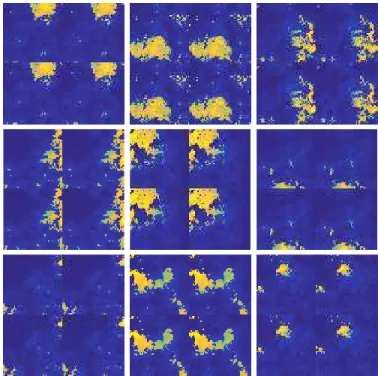
Fig. 3. Abundance maps for the simulated dataset. To demonstrate the effectiveness of our proposed subspace structure constraints, each abundance map consists of four smaller maps built from endmembers in the same subspace.
Fig. 4. Visualization of self-representation matrices for different endmembers.
dataset. The compared hyperspectral unmixing methods in-clude baseline methods VCA-FCLS [16] and NMF [23], sparsity-based methodsL1/2-NMF [28] and graph-regularized L1/2-NMF (GLNMF) [37], spatial information based methods
SGSNMF [41], TV-RSNMF [34], Multilayer NMF method MLNMF [52] and sparsity-constrained deep NMF with total variation (SDNMF-TV) [35]. The results were evaluated with
TABLE I
SADVALUES AND RUNNING TIMES OF THE DIFFERENT METHODS WITH THE SIMULATED DATA.
Method VCA-FCLS NMF L1/2-NMF GLNMF MLNMF SGSNMF TV-RSNMF SDNMF-TV Ours SNR=10dB 0.1315 0.1802 0.1774 0.1809 0.1325 0.1392 0.1193 0.1183 0.1104 SNR=20dB 0.0366 0.0485 0.0344 0.0361 0.0340 0.0348 0.0509 0.0324 0.0297 SNR=30dB 0.0102 0.0152 0.0133 0.0124 0.0201 0.0238 0.0200 0.0105 0.0107 SNR=40dB 0.0024 0.0035 0.0027 0.0026 0.0028 0.0236 0.0037 0.0023 0.0019 Time(s) 72.2 125.4 160.1 187.2 425.8 116.3 190.4 573.5 153.7 TABLE II
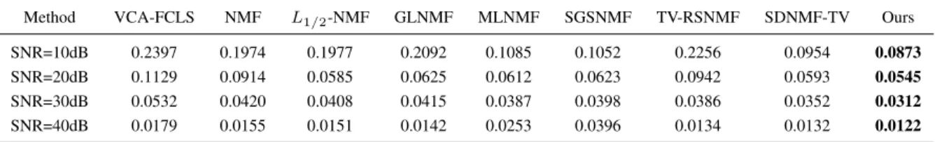
RMSEVALUES OF THE DIFFERENT METHODS WITH THE SIMULATED DATA.
Method VCA-FCLS NMF L1/2-NMF GLNMF MLNMF SGSNMF TV-RSNMF SDNMF-TV Ours SNR=10dB 0.2397 0.1974 0.1977 0.2092 0.1085 0.1052 0.2256 0.0954 0.0873 SNR=20dB 0.1129 0.0914 0.0585 0.0625 0.0612 0.0623 0.0942 0.0593 0.0545 SNR=30dB 0.0532 0.0420 0.0408 0.0415 0.0387 0.0398 0.0386 0.0352 0.0312 SNR=40dB 0.0179 0.0155 0.0151 0.0142 0.0253 0.0396 0.0134 0.0132 0.0122 10-1 10-2 µ 10-3 10-4 10-4 λ 10-2 0.04 0.06 0.055 0.05 0.045 0.035 0.03 100 SAD
(a) SAD results
10-1 10-2 µ 10-3 10-4 10-4 λ 10-2 0.15 0.1 0.05 0.2 100 RMSE (b) RMSE results Fig. 5. Performance of our proposed method with respect to differentλand µwhen SNR = 20 dB.
two commonly used measures to assess the quantitative un-mixing performance: spectral angle distance (SAD) and root-mean-square error (RMSE). The SAD compares the similarity of the estimated signatureAˆk and the groundtruth endmember
Ak, and is defined as:
SADk = arg cos(
ATkAˆk ATk ˆ Ak ) (39)
The RMSE is defined as:
RM SEk= (1 N Sk−Sˆk 2 )1/2 (40) where Sˆk is the groundtruth abundance matrix for the k-th endmember. As stated above, in general, a smaller SAD or RMSE corresponds to a better result.
A. Experiments on Simulated Data
1) Simulated Data: The simulated dataset in this experi-ment was generated according to the Hyperspectral Imagery Synthesis (EIAs) toolbox [53]. It is a free software for users to generate simulated hyperspectral images flexibly by controlling several parameters, such as a certain number of
groundtruth endmembers, the size of the abundance map, spa-tial distribution of materials and different kinds of noises. We randomly selected the endmembers from the USGS mineral spectra library, and generated the corresponding abundance maps according to the Gaussian field. To demonstrate the effectiveness of utilizing the global spatial information, we designed the abundance map by mosaicing four smaller abun-dance matrix together so that each material occurs in different regions of the entire hyperspectral images. Fig. 2 shows 9 selected endmembers and Fig. 3 shows the groundtruth abundance maps built from the 9 endmembers. Here, the simulated dataset has a size of 100×100 pixels and 224 spectral bands.
2) Parameter Analysis: There are two key parameters
λ and µ in our proposed method, where λ measure the sparsity constraints and µ is for subspace structure regu-larization. Firstly, we discuss the influence of these two parameters on the simulated dataset at the circumstance of SNR=20 dB. In this experiment, we changed λ at the in-terval{0.0005,0.001,0.003,0.01,0.05,0.1,0.2,0.3}andµat the interval {0.0001,0.001,0.01,0.1} to test our proposed method. We set parameter τ as 0.001 the same with [34]. The performance of our method for different parameterλand
µis shown in Fig. 5, where (a) displays the SAD results and (b) displays the RMSE results. In general, SAD and RMSE results with respect toλ andµ reveal the same trend. When
λandµboth are near zero, the results are stable. It should be noted that whenλandµboth are zeros, the results correspond to classic NMF. As λ increases it gradually converges to local minima. When λis too large, the results will be worse than NMF. Similar trend can be seen in parameter µ. This indicates the effectiveness of the sparsity constraint as well as the subspace structure constraint. With the proper choice of parameter values, the SAD and RMSE can be significantly decreased. Relatively, parameter µ is more robust than λ, which can be seen more obviously in RMSE results.
(a) (b)
(c)
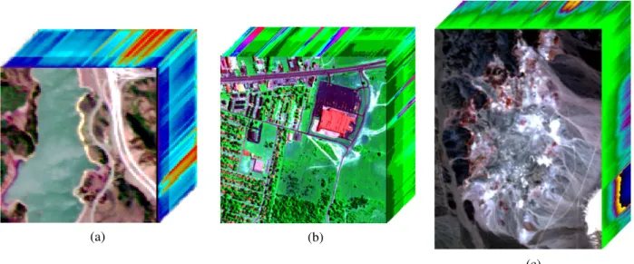
Fig. 6. Three real-world hyperspectral images. (a) HYDICE Jasper Ridge dataset; (b) HYDICE Urban dataset; (c) AVIRIS Cuprite dataset.
value is set as 0.01 for our experiments. As for the sparse regularization parameterλ, we utilize the same strategy in [28] to determine its value:
λe= 1 √ L N X l=1 √ N− kYlk1/kYlk2 √ N−1 (41)
Usually, the optimal parameterλis smaller thanλe. Therefore we can search it at the interval [λe/10, λe]. We set the value of λas 0.1 in the simulated date experiments.
3) Performance Comparisons: Inevitably real-world hyper-spectral images are easily corrupted by noises, which is a great challenge for unmixing. Therefore, different levels of white Gaussian noises was added to the simulated data, which exist in most hyperspectral images. We choose the noise level as {10,20,30,40} dB. Table I presents the SAD values of different methods under different noise levels. We can see that unmixing methods that integrate spatial information like TV-RSNMF and SDNMF-TV have lower SAD values compared to methods that only use sparsity constraints in most cases. This indicates the effectiveness of the utilization of spatial relationships. It can be seen that our method outperforms all the compared methods on different noise levels except when SNR=30dB, as the VCA-FCLS is slightly better than our method. This may be caused by some specific noise which influences the subspace clustering result. In most cases, as the mixed noise increases, the unmixing problem becomes more difficult, our method has more obvious advantages. This verifies that the subspace regularizer, which captures the global spatial relationship, is useful in the hyperspectral unmixing task. Similar results can be seen in Table II, which displays the RMSE values of different methods. In order to demonstrate that the improvement introduced by our method is not at the cost of excessive computational cost, we provide the average running time of different methods. The last row of Table I shows the average running time on different noise levels, we can seen that our method is more efficient than most compared methods that define the distribution structure manually. In
addition, the time cost of our method is significant superior to the multilayer and deep NMF methods.
To further validate the effectiveness of our proposed sub-space structure regularizer, we present the visualization of self-representation matrices of randomly chosen points in different endmembers. As shown in Fig. 4, the lighter areas indicate larger weight in the self-representation matrix. It can be seen that the subspace structure is mostly approximate with the abundance map. Therefore, the learned subspace structure can be used as a robust global spatial prior for unmixing.
B. Experiments on Real Data
In this section, we validate our method on the real-world hyperspectral images. We conducted unmixing experiments on three public hyperspectral datasets: the Hyperspectral Digi-tal Imagery Collection Experiment (HYDICE) Jasper Ridge dataset, the HYDICE Urban dataset, and the AVIRIS Cuprite dataset. Specifically, we obtain the groundtruth following [16]. For the Cuprite dataset, the reference endmember signatures were chosen from the USGS digital spectral library.
1) HYDICE Jasper Ridge dataset: Jasper Ridge is a widely used hyperspectral data for evaluating the unmixing method, which contains 512×614 pixels. There are 224 spectral bands from 380 to 2500 nm. Since the groundtruth of this hyperspectral image is difficult to obtain, we only used a part of image with100×100pixels. Specifically, the first pixel of the chosen part is (105, 269). To avoid the atmospheric effects and dense water vapor problems, we removed related bands (1-3, 108-112, 154-166, 220,224), remaining an image of 198 bands, which is the same with other hyperspectral unmixing methods. As shown in Fig 6(a), the endmembers of Jasper Ridge are “Tree”, “Soil”, “Water” and “Road”.
Quantitative evaluation is presented in Table III which shows the mean SAD and RMSE values of different hyper-spectral unmixing methods. As a representative solution, NMF balances the estimation of endmembers and abundance matrix compared with VCA-FCLS. They both only use non-negative constraints. L1/2-NMF and GLNMF add different kinds of
20 40 60 80 100 20 40 60 80 100 20 40 60 80 100 20 40 60 80 100 20 40 60 80 100 20 40 60 80 100
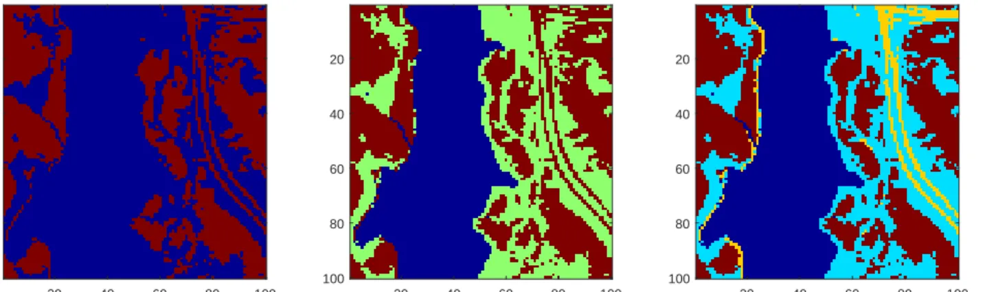
Fig. 7. Clustering results on Jasper Ridge dataset when the number of clusters is set as 2, 3 and 4, respectively.
1 1.5 2 2.5 0 0.1 0.2 0.3 0.5 1 1.5 2 2.5 0 0.5 1 0.5 1 1.5 2 2.5 0 0.2 0.4 0.6 0.8 0.5 1 1.5 2 2.5 0 0.5 1 Wavelength Wavelength Wavelength R ef le ct an ce R ef le ct an ce R ef le ct an ce R ef le ct an ce Water ——Library
——Ours ——Library——Ours
Road ——Library ——Ours ——Library ——Ours Wavelength Tree Soil 0.5
Fig. 8. Comparison of the library spectra with the endmember signatures extracted by our method on the Jasper Ridge dataset.
sparsity constraints and obtain better results. This may because sparse constraints is more effective for unmixing problem, and it can detect expressive endmembers [54]. However, these methods often have poor RMSE performance since they only focus on endmembers. The utilization of spatial information solves this problem to a certain degree. Neighbor-based TV-RSNMF and deep NMF with total variation SDNMF-TV both have great performance, and SDNMF-TV is slightly better than the other compared methods. It can be seen from Table III that our proposed method that learns spatial information from original images rather than design manually achieve better performance for real-world hyperspectral unmixing. In gen-eral, our proposed method achieves the lowest mean SAD values as well as the lowest mean RMSE compared with the other methods. This validates the superiority of the proposed subspace regularizer.
The qualitative unmixing results are shown in Fig. 8 and Fig. 9. From Fig. 8, we can see that the endmember signa-tures extracted by our method is almost coincident with the reference signatures obtained from the spectral library. Fig. 9
Fig. 9. Abundance maps of 4 different endmembers obtained using our method on the Jasper Ridge dataset. From left to right and from top to bottom are Water, Soil, Road and Tree, respectively.
displays the abundance map obtained by our method. The corresponding endmember is illustrated with dark pixels. From Fig. 9, we can see the results quite agree with the four targets, “Water”, “Soil”, “Road” and “Tree”, respectively.
Simultaneously, we obtained the clustering results. Since our method can jointly learn the subspace structure of the dataset, then the clustering result can be obtained by a standard spectral clustering algorithm. Fig. 7 shows the results when the number of clusters is set as 2, 3 and 4 respectively. It can be seen that the clustering results conform to the real image intuitively.
2) HYDICE Urban dataset: HYDICE Urban dataset is another widely used hyperspectral image. It includes307×307
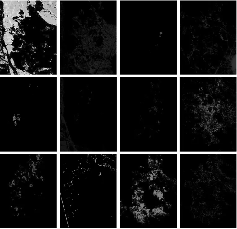
Fig. 10. Abundance maps of 12 different endmembers obtained using our method on the Cuprite dataset. From left to right and from top to bottom are Sphene, Andradite, Muscovite, Montmorillonite, Buddingtonite, Kaolinite-2, Alunite, Dumortierite, Kaolinite-1, Pyrope, Chalcedony and Nontronite, respectively.
400-2500 nm. Here, noisy bands (1-4) and water-absorption (76, 87, 101-111, 136-153, and 198-210) bands were removed, resulting in an image of 162 bands. The groundtruth in-cludes six endmembers: “Asphalt”, “Tree”, “Grass”, “Roof#1”, “Roof#2”, and “Concrete road” as shown in Fig 6(b).
Similar to the previous experiment, Table IV shows the mean SAD and RMSE values. We observe that the proposed subspace learning regularized NMF method outperforms al-l the other methods. In this experiment, TV-RSNMF and SDNMF-TV that use spatial information obtain slightly better results than sparse-based methods. This indicates the
effec-tiveness of spatial relationships for complex image unmixing.
3) AVIRIS Cuprite dataset: Cuprite dataset contains 224 spectral bands cover the range of 400-2500nm. A total of 188 bands remained by removing noisy bands (1-2 and 221-224) and water-vapor absorption bands (104-113 and 148-167). In this experiment, a spatial size of 250×191 was tailored, which contains 14 kinds of minerals [16]. Since there are only tiny differences between signatures of several minerals, the estimated number of endmembers was reduced to 12 for the unmixing. It is shown in Fig 6(c).
Table V compares the SAD results of different hyperspectral unmixing methods. We use bold to indicate the best and
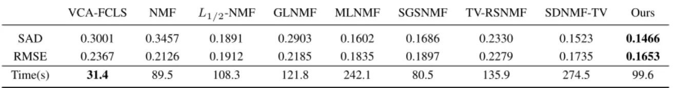
TABLE III
SADANDRMSEVALUES AND RUNNING TIMES OF DIFFERENT METHODS ON THEJASPERRIDGE DATASET. VCA-FCLS NMF L1/2-NMF GLNMF MLNMF SGSNMF TV-RSNMF SDNMF-TV Ours SAD 0.3001 0.3457 0.1891 0.2903 0.1602 0.1686 0.2330 0.1523 0.1466 RMSE 0.2367 0.2126 0.1912 0.2185 0.1835 0.1897 0.2279 0.1735 0.1653
Time(s) 31.4 89.5 108.3 121.8 242.1 80.5 135.9 274.5 99.6
TABLE IV
SADANDRMSEVALUES AND RUNNING TIMES OF DIFFERENT METHODS ON THEURBAN DATASET.
VCA-FCLS NMF L1/2-NMF GLNMF MLNMF SGSNMF TV-RSNMF SDNMF-TV Ours SAD 0.3966 0.3721 0.2674 0.3129 0.2431 0.2410 0.2559 0.2375 0.2307 RMSE 0.2764 0.2417 0.1726 0.2274 0.1706 0.1744 0.1904 0.1642 0.1593
Time(s) 124.3 253.2 341.8 352.6 895.2 203.4 318.3 975.3 289.4
TABLE V
SADVALUES AND RUNNING TIMES OF DIFFERENT METHODS ON THECUPRITE DATASET.
Method VCA-FCLS NMF L1/2-NMF GLNMF MLNMF SGSNMF TV-RSNMF SDNMF-TV Ours Alunite 0.1094 0.1164 0.1245 0.1090 0.0958 0.1072 0.1032 0.0980 0.1099 Andradite 0.0568 0.0806 0.0732 0.0665 0.0743 0.1062 0.0810 0.0673 0.0711 Buddingtonite 0.1215 0.3762 0.1173 0.1130 0.1319 0.1197 0.1141 0.1141 0.1059 Dumortierite 0.0759 0.1216 0.0974 0.0798 0.0856 0.0761 0.0997 0.1015 0.0959 Kaolinite-1 0.0985 0.1072 0.1356 0.0994 0.0991 0.0778 0.0771 0.1075 0.0963 Kaolinite-2 0.0603 0.0901 0.0549 0.0624 0.0775 0.0844 0.0489 0.0753 0.0740 Muscovite 0.2130 0.2739 0.1443 0.1002 0.0745 0.1498 0.1427 0.0989 0.1306 Montmorillonite 0.0983 0.0922 0.0535 0.1030 0.0921 0.0595 0.0599 0.0800 0.0616 Nontronite 0.0733 0.4640 0.0744 0.0733 0.1177 0.1254 0.0702 0.1277 0.0784 Pyrope 0.1711 0.1817 0.0931 0.2455 0.1045 0.0605 0.0705 0.1118 0.0610 Sphene 0.0577 0.1155 0.2618 0.0552 0.0508 0.3159 0.2737 0.0642 0.1930 Chalcedony 0.0992 0.0992 0.0698 0.1450 0.1387 0.0980 0.1207 0.1477 0.0988 Mean 0.1022 0.1765 0.1083 0.1044 0.1001 0.1147 0.1055 0.0995 0.0981 Time(s) 53.2 102.1 153.5 169.3 410.2 93.5 174.5 493.5 142.8
underline for the second best performance for each end-member. As shown in Table V, our method outperforms the compared methods for the mean SAD values. Different methods are good at estimating different endmembers, this might be because most of the endmembers in this dataset are tiny and fragmented, the spatial structure is not so obvious and unified. For endmembers like “Buddingtonite”, “pyrope” and “Chalcedony”, our proposed method has great advantages. Since the Cuprite dataset has no groundtruth, we only show the grayscale abundance maps obtained by our method in Fig. 10. Compared to the original image shown in Fig 6(c), the results can be verified intuitively.
V. CONCLUSION
In this paper, we have proposed a spatial information based NMF by learning the subspace structure from the original image for blind hyperspectral unmixing. The presented model effectively exploits the subspace structure of the abundance map to constrain the NMF method. We first incorporate the subspace structure regularizer into the sparse NMF model as a spatial prior to improve the unmixing performance. The
learned subspace structure can capture the global distribu-tion of materials in different image regions. Then, we have integrated the spectral-spatial based unmixing and subspace structure learning in a single unified framework and presented a multiplicative iterative method to optimize it. We compared our method with plenty classical and state-of-the-art NMF based hyperspectral unmixing methods on both simulated and real-word HSI datasets. Both quantitative and qualitative results demonstrate the effectiveness of our method.
REFERENCES
[1] X. Bai, H. Zhang, and J. Zhou, “Vhr object detection based on structural feature extraction and query expansion,”IEEE Transactions on Geoscience and Remote Sensing, vol. 52, no. 10, pp. 6508–6520, 2014.
[2] J. Liang, J. Zhou, Y. Qian, L. Wen, X. Bai, and Y. Gao, “On the sampling strategy for evaluation of spectral-spatial methods in hyperspectral image classification,”IEEE Transactions on Geoscience and Remote Sensing, vol. 55, no. 2, pp. 862–880, 2016.
[3] S. Mei, J. Hou, J. Chen, L.-P. Chau, and Q. Du, “Simultaneous spatial and spectral low-rank representation of hyperspectral images for classification,”IEEE Transactions on Geoscience and Remote Sensing, vol. 56, no. 5, pp. 2872–2886, 2018.
[4] M. Zhang, W. Li, and Q. Du, “Diverse region-based CNN for hyper-spectral image classification,”IEEE Transactions on Image Processing, vol. 27, no. 6, pp. 2623–2634, 2018.
[5] X. Bai, F. Xu, L. Zhou, Y. Xing, L. Bai, and J. Zhou, “Nonlocal similarity based nonnegative tucker decomposition for hyperspectral image denoising,”IEEE Journal of Selected Topics in Applied Earth Observations and Remote Sensing, vol. 11, no. 3, pp. 701–712, 2018. [6] J. Li, Y. Li, R. Song, S. Mei, and Q. Du, “Local spectral similarity
preserving regularized robust sparse hyperspectral unmixing,” IEEE Transactions on Geoscience and Remote Sensing, vol. 57, no. 10, pp. 7756–7769, 2019.
[7] D. Wang, Z. Shi, and X. Cui, “Robust sparse unmixing for hyperspec-tral imagery,”IEEE Transactions on Geoscience and Remote Sensing, vol. 56, no. 3, pp. 1348–1359, 2017.
[8] Y. E. Salehani, S. Gazor, and M. Cheriet, “Sparse hyperspectral unmix-ing via heuristiclp-norm approach,”IEEE Journal of Selected Topics
in Applied Earth Observations and Remote Sensing, vol. 11, no. 4, pp. 1191–1202, 2017.
[9] L. Tong, J. Zhou, Y. Qian, X. Bai, and Y. Gao, “Nonnegative-matrix-factorization-based hyperspectral unmixing with partially known end-members,” IEEE Transactions on Geoscience and Remote Sensing, vol. 54, no. 11, pp. 6531–6544, 2016.
[10] R. Heylen, M. Parente, and P. Gader, “A review of nonlinear hyperspec-tral unmixing methods,”IEEE Journal of Selected Topics in Applied Earth Observations and Remote Sensing, vol. 7, no. 6, pp. 1844–1868, 2014.
[11] B. Yang, B. Wang, and Z. Wu, “Nonlinear hyperspectral unmixing based on geometric characteristics of bilinear mixture models,”IEEE Transactions on Geoscience and Remote Sensing, vol. 56, no. 2, pp. 1–21, 2017.
[12] F. J. Garca-Haro, M. A. Gilabert, and J. Meli, “Linear spectral mixture modelling to estimate vegetation amount from optical spectral data,”
International Journal of Remote Sensing, vol. 17, no. 17, p. 28, 1996. [13] J. W. Boardman, “Automating spectral unmixing of AVIRIS data using
convex geometry concepts,” 1994, pp. 11–14.
[14] M. E. Winter, “N-FINDr: An algorithm for fast autonomous spectral endmember determination in hyperspecral data,”Proceedings of SPIE -The International Society for Optical Engineering, vol. 3753, pp. 266– 275, 1999.
[15] A. Zymnis, S. J. Kim, J. Skaf, M. Parente, and S. Boyd, “Hyperspectral image unmixing via alternating projected subgradients,” in Asilomar Conference on, 2008.
[16] J. M. P. Nascimento and J. M. B. Dias, “Vertex component analysis: A fast algorithm to unmix hyperspectral data,”IEEE Transactions on Geoscience and Remote Sensing, vol. 43, no. 4, pp. 898–910, 2005. [17] J. Wang and C. I. Chang, “Applications of independent component
analysis in endmember extraction and abundance quantification for hyperspectral imagery,”IEEE Transactions on Geoscience and Remote Sensing, vol. 44, no. 9, pp. 2601–2616, 2006.
[18] M. Craig, “Minimum volume transforms for remotely sensed data,”
IEEE Transactions on Geoscience and Remote Sensing, vol. 32, no. 3, pp. 542–552, 1994.
[19] J. Huang, T.-Z. Huang, L.-J. Deng, and X.-L. Zhao, “Joint-sparse-blocks and low-rank representation for hyperspectral unmixing,”IEEE Transactions on Geoscience and Remote Sensing, vol. 57, no. 4, pp. 2419–2438, 2019.
[20] Y. Su, J. Li, A. Plaza, A. Marinoni, P. Gamba, and S. Chakravortty, “DAEN: Deep autoencoder networks for hyperspectral unmixing,”IEEE Transactions on Geoscience and Remote Sensing, vol. 57, no. 7, pp. 4309–4321, 2019.
[21] F. Khajehrayeni and H. Ghassemian, “Hyperspectral unmixing using deep convolutional autoencoders in a supervised scenario,”IEEE Journal of Selected Topics in Applied Earth Observations and Remote Sensing, vol. 13, pp. 567–576, 2020.
[22] R. A. Borsoi, T. Imbiriba, and J. C. M. Bermudez, “Deep generative end-member modeling: An application to unsupervised spectral unmixing,”
IEEE Transactions on Computational Imaging, 2019.
[23] D. D. Lee and H. S. Seung, “Learning the parts of objects by non-negative matrix factorization,”Nature, vol. 401, no. 6755, p. 788, 1999. [24] D. Lee and S. Seung, “Algorithms for non-negative matrix factorization,” inAdvances in Neural Information Processing Systems, 2001, pp. 556– 562.
[25] A. Cichocki, R. Zdunek, A. H. Phan, and S. I. Amari, Nonnegative Matrix and Tensor Factorizations: Applications to Exploratory Multi-Way Data Analysis and Blind Source Separation, 2009.
[26] P. Hoyer, “Non-negative matrix factorization with sparseness con-straints,”Journal of Machine Learning Research, vol. 5, no. 1, pp. 1457– 1469, 2004.
[27] P. O. Hoyer, “Non-negative sparse coding,” inProceedings of the 12th IEEE Workshop on Neural Networks for Signal Processing. IEEE, 2002, pp. 557–565.
[28] Y. Qian, S. Jia, J. Zhou, and A. Robles-Kelly, “Hyperspectral unmixing via l1/2 sparsity-constrained nonnegative matrix factorization,” IEEE
Transactions on Geoscience and Remote Sensing, vol. 49, no. 11, pp. 4282–4297, 2011.
[29] Y. Ma, C. Li, X. Mei, C. Liu, and J. Ma, “Robust sparse hyperspectral unmixing with l2,1 norm,” IEEE Transactions on Geoscience and
Remote Sensing, vol. 55, no. 3, pp. 1227–1239, 2017.
[30] D. Kong, C. Ding, and H. Huang, “Robust nonnegative matrix factor-ization usingl2,1-norm,” inProceedings of the 20th ACM international
conference on Information and knowledge management, 2011, pp. 673– 682.
[31] W. He, H. Zhang, and L. Zhang, “Sparsity-regularized robust non-negative matrix factorization for hyperspectral unmixing,”IEEE Journal of Selected Topics in Applied Earth Observations and Remote Sensing, vol. 9, no. 9, pp. 4267–4279, 2016.
[32] R. Huang, X. Li, and L. Zhao, “Spectral–spatial robust nonnegative matrix factorization for hyperspectral unmixing,”IEEE Transactions on Geoscience and Remote Sensing, vol. 57, no. 10, pp. 8235–8254, 2019. [33] M. D. Iordache, J. M. Bioucas-Dias, and A. Plaza, “Total variation spatial regularization for sparse hyperspectral unmixing,”IEEE Transac-tions on Geoscience and Remote Sensing, vol. 50, no. 11, pp. 4484–4502, 2012.
[34] H. Wei, H. Zhang, and L. Zhang, “Total variation regularized reweighted sparse nonnegative matrix factorization for hyperspectral unmixing,”
IEEE Transactions on Geoscience and Remote Sensing, vol. 55, no. 99, pp. 1–13, 2017.
[35] X.-R. Feng, H.-C. Li, J. Li, Q. Du, A. Plaza, and W. J. Emery, “Hy-perspectral unmixing using sparsity-constrained deep nonnegative matrix factorization with total variation,”IEEE Transactions on Geoscience and Remote Sensing, vol. 56, no. 10, pp. 6245–6257, 2018.
[36] X. Liu, X. Wei, B. Wang, and L. Zhang, “An approach based on constrained nonnegative matrix factorization to unmix hyperspectral data,”IEEE Transactions on Geoscience and Remote Sensing, vol. 49, no. 2, pp. 757–772, 2011.
[37] X. Lu, H. Wu, Y. Yuan, P. Yan, and X. Li, “Manifold regularized sparse NMF for hyperspectral unmixing,” IEEE Transactions on Geoscience and Remote Sensing, vol. 51, no. 5, pp. 2815–2826, 2013.
[38] W. Dong, X. Li, L. Zhang, and G. Shi, “Sparsity-based image denoising via dictionary learning and structural clustering,” inCVPR 2011. IEEE, 2011, pp. 457–464.
[39] X. Lu, H. Wu, and Y. Yuan, “Double constrained nmf for hyperspectral unmixing,” IEEE Transactions on Geoscience and Remote Sensing, vol. 52, no. 5, pp. 2746–2758, 2013.
[40] S. Khoshsokhan, R. Rajabi, and H. Zayyani, “Clustered multitask non-negative matrix factorization for spectral unmixing of hyperspectral data,” Journal of Applied Remote Sensing, vol. 13, no. 2, p. 026509, 2019.
[41] X. Wang, Y. Zhong, L. Zhang, and Y. Xu, “Spatial group sparsity reg-ularized nonnegative matrix factorization for hyperspectral unmixing,”
IEEE Transactions on Geoscience and Remote Sensing, vol. 55, no. 11, pp. 6287–6304, 2017.
[42] H. Zhang, Z. Han, L. Zhang, and P. Li, “Spectralspatial sparse subspace clustering for hyperspectral remote sensing images,”IEEE Transactions on Geoscience and Remote Sensing, vol. 54, no. 6, pp. 3672–3684, 2016. [43] L. Zhou, X. Bai, X. Liu, J. Zhou, and E. R. Hancock, “Learning binary code for fast nearest subspace search,”Pattern Recognition, vol. 98, p. 107040, 2020.
[44] P. Ji, T. Zhang, H. Li, M. Salzmann, and I. Reid, “Deep subspace clustering networks,” in Advances in Neural Information Processing Systems, 2017, pp. 24–33.
[45] L. Zhou, B. Xiao, X. Liu, J. Zhou, E. R. Hancock et al., “Latent distribution preserving deep subspace clustering,” in28th International Joint Conference on Artificial Intelligence, 2019.
[46] G. Liu, Z. Lin, and Y. Yu, “Robust subspace segmentation by low-rank representation,” inProceedings of the 27th international conference on machine learning, 2010, pp. 663–670.
[47] G. Liu, Z. Lin, S. Yan, J. Sun, Y. Yu, and Y. Ma, “Robust recovery of subspace structures by low-rank representation,”IEEE Transactions on Pattern Analysis and Machine Intelligence, vol. 35, no. 1, pp. 171–184, 2012.
[48] N. Keshava, “A survey of spectral unmixing algorithms,”Lincoln labo-ratory journal, vol. 14, no. 1, pp. 55–78, 2003.
[49] F. Xiong, J. Zhou, and Y. Qian, “Material based object tracking in hyperspectral videos,”IEEE Transactions on Image Processing, vol. 29, no. 1, pp. 3719–3733, 2020.
[50] J. F. Cai, E. J. Cands, and Z. Shen, “A singular value thresholding algorithm for matrix completion,”Siam Journal on Optimization, vol. 20, no. 4, pp. 1956–1982, 2008.
[51] D. C. Heinz et al., “Fully constrained least squares linear spectral mixture analysis method for material quantification in hyperspectral imagery,”IEEE transactions on geoscience and remote sensing, vol. 39, no. 3, pp. 529–545, 2001.
[52] R. Rajabi and H. Ghassemian, “Spectral unmixing of hyperspectral imagery using multilayer NMF,”IEEE Geoscience and Remote Sensing Letters, vol. 12, no. 1, pp. 38–42, 2014.
[53] “Hyperspectral imagery synthesis (eias) toolbox.”Grupo de Inteligencia Computacional, Universidad del Pas Vasco / Euskal Herriko Unibertsi-tatea (UPV/EHU), Spain.
[54] S. Z. Li, X. W. Hou, H. J. Zhang, and Q. S. Cheng, “Learning spatially localized, parts-based representation,” inProceedings of the 2001 IEEE Computer Society Conference on Computer Vision and Pattern Recognition, vol. 1. IEEE, 2001, pp. I–I.
Lei Zhoureceived the Bachelor’s degree in 2016 from the School of Mathematics and Systems Sci-ence, Beihang University, Beijing, China, where he is currently working toward the Ph.D. degree at the School of Computer Science and Engineering.
His current research interests include machine learning, computer vision, and remote sensing image processing.
Xueni Zhang received the Bachelor’s degree in 2017 from the College of Computer Science and Technology, Jilin University, Jilin, China, and re-ceived the Master of Engineering degree in 2020 from the School of Computer Science and Engineer-ing, Beihang University, BeijEngineer-ing, China.
Her research interests include computer vision and remote sensing image processing.
Jianbo Wangis currently an undergraduate at the First Clinical Medical College of Nanchang Univer-sity, Jiangxi, China.
His research interests include machine learning and image processing.
Xiao Baireceived the B.Eng. degree in computer science from Beihang University, Beijing, China, in 2001, and the Ph.D. degree in computer science from the University of York, York, U.K., in 2006.
He was a Research Officer (Fellow, Scientist) with the Computer Science Department, University of Bath, until 2008. He is currently a Full Pro-fessor with the School of Computer Science and Engineering, Beihang University. He has authored or co-authored more than 60 papers in journals and refereed conferences. His current research interests include pattern recognition, image processing, and remote sensing image analysis.
Lei Tong received the B.E. degree in measure-ment and control technology and instrumeasure-mentation, the M.E. degree in measurement technology and automation devices from Beijing Jiaotong Univer-sity, Beijing, China, in 2010 and 2012, respectively. He received the Ph.D. degree in Engineering from Griffith University, Brisbane, Australia, in 2016. Currently, he is a Lecturer with Faculty of Informa-tion Technology, Beijing University of Technology, Beijing, China.
His current research interests include signal and image processing, pattern recognition, and remote sensing.
Liang Zhangreceived the B.Eng. degree in comput-er science from Beihang Univcomput-ersity, Beijing, China, in 2001, and the Ph.D. degree in computer science from Beihang University, Beijing, China, in 2007.
His current research interests include machine learning, computer vision, image processing.
Jun Zhou received the B.S. degree in computer science and the B.E. degree in international business from the Nanjing University of Science and Technol-ogy, Nanjing, China, in 1996 and 1998, respectively; the M.S. degree in computer science from Concordia University, Montreal, QC, Canada, in 2002; and the Ph.D. degree in computing science from the University of Alberta, Edmonton, AB, Canada, in 2006.
He was a Research Fellow with the Research School of Computer Science, Australian National University, Canberra, ACT, Australia, and a Researcher with the Canberra Research Laboratory, NICTA, Canberra, ACT, Australia. In June 2012, he joined the School of Information and Communication Technology, Griffith University, Nathan, QLD, Australia, where he is currently an Associate Pro-fessor. His research interests include pattern recognition, computer vision, and spectral imaging with their applications in remote sensing and environmental informatics.
Edwin Hancock holds a BSc degree in physics (1977), a PhD degree in high-energy physics (1981) and a D.Sc. degree (2008) from the University of Durham, and a doctorate Honoris Causa from the University of Alicante in 2015. He is Professor in the Department of Computer Science, where he leads a group of some faculty, research staff, and PhD students working in the areas of computer vision and pattern recognition. His main research interests are in the use of optimization and probabilistic methods for high and intermediate level vision. He is a fellow of the International Association for Pattern Recognition and the IEEE. He is currently Editor-in-Chief of the journal Pattern Recognition, and was founding Editor-in-Chief of IET Computer Vision from 2006 until 2012. He has also been a member of the editorial boards of the journals IEEE Transactions on Pattern Analysis and Machine Intelligence, Pattern Recognition, Computer Vision and Image Understanding, Image and Vision Computing, and the International Journal of Complex Networks.