Joint Panel Sizing and Appointment Scheduling
in Outpatient Care
Christos Zacharias, Mor Armony
Department of Information, Operations & Management Sciences, Stern School of Business, New York University, New York, NY 10012.
{czachari,marmony}@stern.nyu.edu
Patients nationwide experience difficulties in accessing medical appointments in a timely manner due to long backlogs. Meanwhile, patients do not always show up for their scheduled services, with significant no-show rates. Unattended appointments result in under-utilization of a clinic’s valuable resources, and limit the access for other patients who could have filled the missed slots. Medical practices aim to utilize their valuable resources efficiently, provide timely access to care, and at the same time they strive to provide short waits for patients present at the medical facility. We study the joint problem of determining the panel size of a medical practice and the number of offered appointment slots per day, so that patients do not face long backlogs and the clinic is not overcrowded.
We explicitly model the two separate time scales involved in accessing medical care: appointment delay (order of days, weeks) and clinic delay (order of minutes, hours). We analyze the two queueing systems associated with each type of delay, and provide explicit expressions for the performance measures of interest based on diffusion approximations. In our analysis we capture many features of the complex reality of outpatient care, including patients’ non-punctuality, no-shows, balking behavior, and stochastic service times. Two additional distinctive characteristics of this study are the balking behavior of the patients who face long appointment backlogs, and the transient-state analysis of the clinic delay, which allow the study of a system with traffic intensity greater than one.
Concerning the panel sizing and appointment scheduling decisions, our analysis provides theoretical and numerical support that the two-variable optimization problem reduces to a single variable-one, and either an “Open Access” policy is optimal, or supply and demand are perfectly matched and are both very small (“Limited Access” regime). Under our Open Access regime, the clinic offers as many appointment slots as possible per day, and the optimal panel size depends on the clinic’s characteristics. A solution within the Limited Access regime arises when the service times are long, and the patients are very sensitive to the appointment delay.
Key words: healthcare management, patient flow management, panel-size, appointment scheduling, no-shows, balking, diffusion approximations, open access
1. Introduction
Patients nationwide experience difficulties in accessing medical appointments in a timely manner due to long backlogs. Merritt (2011), by surveying 1162 medical offices in 15 US metropolitan areas, found that the waiting time to get an appointment averages 20.5 days and depends on the
specialty: 15.5 for cardiology, 22.1 days for dermatology, 27.5 days for obstetrics/gynecology, 16.8 days for orthopedic surgery, 20.3 days for family practice.
The healthcare delivery system also suffers from patient no-show behavior. No-shows in medical care have been well documented, with no-show rates reaching up to 60%, depending on the clinic’s characteristics (Cayirli et al. (2006)). Defife et al. (2010) report a 21% no-show rate in psychother-apy appointments, Dreiher et al. (2008) report a 30% proportion of nonattendance in an outpatient obstetrics and gynecology clinic, Rust et al. (1995) report a 31% appointment failure rate in pedi-atric resident continuity clinics nationally. Unattended appointments result in under-utilization of a clinic’s valuable resources, and limit the access for other patients who could have filled the missed slots.
Medical practices aim to utilize their valuable resources efficiently, provide timely access to care, and at the same time they strive to provide short waits for patients present at the medical facility. Appointment overbooking is one operational strategy employed by healthcare providers that addresses both the issues of long appointment backlogs and patient no-shows. On the other hand, overbooking potentially results in an overcrowded clinic, with increased patients’ waits and physicians’ overtime. As argued in Krueger (2009): “Patient time is an important input in the healthcare system. Failing to take account of patient time leads us to exaggerate the productivity of the health care sector, and to understate the cost of healthcare”. On the flip side, LaGanga and Lawrence (2007) show that a sensible practice of appointment overbooking can significantly improve a clinic’s performance by increasing patients’ access and improving the physicians’ productivity.
Many papers have appeared in the literature on appointment scheduling. Cayirli and Veral (2003), Gupta and Denton (2008) provide literature surveys and overviews of the research chal-lenges. One way to classify the existing literature is with respect to the type of delay addressed: appointment delay and clinic delay. Appointment delay is defined as the time gap between the appointment request and the offered appointment. Clinic delay is the physical waiting time expe-rienced by the patients once they arrive at the medical facility. Very few studies consider the appointment delay, and to the best of our knowledge, ours is the first to consider both jointly, and to provide explicit expressions for the performance measures of interest.
There are two main levers that healthcare providers can use to manage their patient flow, and consequently their productivity and the two aforementioned types of delay. The first one comes by controlling the demand side through their “Panel Size”, i.e., the size of the population of patients who receive their care from the practice on some regular basis. The second lever is the appointment availability, i.e., the number of offered appointment slots per day. It is clear that an increased panel size comes along with a more congested clinic and longer appointment delays. Concerning the number of appointments to offer per day, as demonstrated later on in this paper, it is unclear
as to how it affects the appointment delay. Intuitively, one would expect the appointment backlog to be decreasing in the daily rate that the clinic offers appointment slots. But note that there is a second order effect as well, induced by the patients’ balking behavior: the more the appointment availability, the more likely it is that a patient will have access to an appointment slot of her preference and not balk.
In this paper, we study the joint problem of determining the panel size of a medical practice and the number of offered appointments per day, so that patients do not face long backlogs, and the medical facility is not overcrowded. Our analysis provides theoretical and numerical support that either an “Open Access” policy is optimal in outpatient scheduling, or supply and demand are perfectly matched and are both very small.
The rest of the paper is structured as follows. In §2 we discuss the related literature. In §3 we introduce the modeling framework and define the optimization problem under study. In§4 and §5 we analyze the two queueing systems associated with each time scale, and we provide analytical expressions for the performance measures of interest based on diffusion approximations. In §6 we optimize the daily net benefit of the medical facility from providing care to patients, based on the expressions derived in §4 and§5, with respect to the panel size and the appointment availability. Finally, in §7, we conclude and present future research directions. All the proofs appear in the Appendix.
2. Related Literature
There is an extensive literature on appointment scheduling, mostly motivated by healthcare appli-cations. The vast majority of the literature considers the clinic delay and studies the trade-offs between the benefits of efficient physician utilization and the costs of patients’ waiting time and physician’s overtime. Hall (2012) provides a comprehensive review of models and methods used for scheduling the delivery of patient care for all parts of the healthcare system. The analysis may be based on anyone from a variety of approaches, including stochastic programming, queueing models, and simulation. Kaandorp and Koole (2007), Hassin and Mendel (2008), Klassen and Yoogalingam (2009), Robinson and Chen (2010), LaGanga and Lawrence (2012), Zacharias and Pinedo (2013) are some recent works that address the question of how to optimally allocate the offered appoint-ment slots throughout the working day, taking into account patients’ no-show behavior. There are no analytical expressions for the patients’ waits and physicians’ overtime. Only under certain assumptions on the service times’ distribution (deterministic or exponential), and by assuming punctual patients, recursive expressions can be derived.
In contrast to the aforementioned stream of literature, we do not consider the optimal intra-day scheduling per se. By assuming that patients arrive at the clinic according to a renewal process,
and that the service times are iid random variables, we provide analytical expressions for the performance measures of interest based on diffusion approximations. The renewal arrival process captures both patients’ non-punctuality, and no-show behavior.
Very few works consider the appointment delay and the panel sizing problem. Green and Savin (2008) and Liu and Ziya (2013) model the appointment system as a single server queue and take under consideration state dependent no-show behavior. Green and Savin (2008) develop expressions for the appointment delays, by considering both M/M/1/K and M/D/1/K queueing models in steady state, and identify proper panel sizes for medical practices that aim to implement an Open Access policy. Liu and Ziya (2013) model the appointment queue as an M/M/1 service system in steady state, and address the problem of taking joint optimal panel sizing and overbooking decisions. Finally, Green et al. (2007) propose a probabilistic model to study the timeliness of care, while considering the constraints on physicians working hours. They find that supply of medical appointments must be sufficiently higher than the demand, in order to sustain Open Access scheduling.
Balasubramanian et al. (2010, 2012) analyze the tradeoffs between timely access and continuity of care. In the former study they propose a redesign of physicians’ panel-composition, based on data derived from a large group practice. In the latter work they investigate the value of flexibility in medical practices by addressing the problem of how to optimally allocate the available physicians’ slots among pre-scheduled and Open Access appointments.
In this paper, we study the joint problem of determining the panel size of a medical practice and the number of offered appointments per day, so that patients do not face long backlogs, and the medical facility is not overcrowded. To the best of our knowledge, our work is the first to explicitly model the two separate time scales involved in accessing outpatient medical care: appointment delay (order of days, weeks) and clinic delay (order of minutes, hours), and to provide explicit expressions for the performance measures of interest based on diffusion approximations. The importance of considering the separate time scales involved in different sectors of healthcare delivery has also been discussed in Armony et al. (2011), Dai and Shi (2013), and Luo et al. (2013). Two additional distinctive characteristics of this study are the state-dependent balking behavior of the patients who face long appointment backlogs, and the transient-state analysis of the in-clinic queue, which bear unique technical challenges, and allow the study of a system with traffic intensity greater than one.
Finally, we point out that the appointment scheduling problem, and specifically the number of offered appointments per day component, has natural connection with the control of perishable goods inventory (Bulinskaya (1964), Abad (1996)). Consider the multi-period inventory control
problem of a product that perishes after one period, random demand, and state-depended back-ordering. Positive inventory at the end of the period corresponds to unused time slots, which perish and cannot be used in future periods, and negative inventory corresponds to a backlog of appointments.
3. Problem Formulation
In this section we introduce the modeling framework and we formulate the optimization problem under study. Figure 1 depicts a schematic representation of the model.
Consider a clinic with a panel of sizeN patients, which triggers a demand for scheduled appoint-ments via an appointment book. The patients’ decision whether to join the backlog depends on its state. Let Aa(t) be the cumulative number of patients that have booked an appointment in [0, t],
and Wa(t) be the workload (or equivalently the offered waiting time) of the appointment book at
time t. No-shows are treated as follows. A patient who does not show up in the clinic, occupies a position in the appointment book until the day of her scheduled appointment, and the backlog dynamics are unaffected.
Each day, depending on the state of the appointment book, a number of patients is scheduled to arrive at the clinic. In contrast with the appointment book, the clinic starts empty at the beginning of each period. The length of a regular working day isThours, during which the scheduled appointments are allocated. The server continues to work overtime as well, beyond T, until the queue empties. Let Ac(t) be the cumulative number of clinic arrivals in [0, t], subject to no-show
behavior, and Wc(t) be the workload of the clinic at timet.
We are interested in optimizing the long run average daily net benefit of a medical facility from providing care to patients, with respect to the panel size,N, and the number of offered appointment slots per working day, s. There is a reward r generated per patient served. For the appointment book we consider a holding costcaper time unit that each patient who joins the backlog has to wait
for her scheduled appointment. There are two types of costs associated with the in-clinic queue: a waiting costcw per time unit that each patient has to wait to see a physician, and an overtime cost co per time unit that the clinic has to operate overtime. The optimization problem under study is
max N,s tlim→∞ 1 t ( rAc(t)−c a ∫ t 0 Wa(τ)dAa(τ)−c w ∫ t 0 Wc(τ)dAc(τ)−c o ∫ t 0 1{Wc(τ)>0, τ overtime}dτ ) . (1)
In§4 and§5 we analyze the two queueing systems associated with the two time scales involved in accessing medical care, and, based on diffusion approximations, we provide an analytical expression for the objective function in (1).
Figure 1 Schematic representation of the model.
4. The Appointment Book
First, we are interested in characterizing the evolution of the appointment backlog as a function of the panel size and the number of offered slots per working day, disregarding the intra-day dynamics. In order to obtain a tractable expression for the appointment delay, we develop a heavy traffic diffusion approximation.
The supply of medical appointments is s slots per day. Requests for appointments arrive at a rate λper day, with λbeing an increasing function of the panel size. For instance, as pointed out in Robinson and Chen (2010), if the panel size of a clinic is N, and each patient independently requests an appointment for any given period with a small probability q, then the arrival rate of appointment requests isλ=N q per day, and the number of patients requesting appointments will follow the binomial distribution with parametersN andq, which converges to a Poisson distribution with meanN q asN→ ∞.
More generally, we assume that appointment requests arrive to the appointment book according to a renewal process. The patients’ decision of whether to book an appointment or not depends on the state of the appointment book: the less congested the latter, the more likely it is that a patient will have access to a slot of her preference. Each patient requires service of 1 time slot, and
s appointment slots are offered each working day. Each day the appointment book provides the clinic with a schedule of up tospatients.
We model the appointment book as a GI/D/1 queue with batch services and state dependent balking. The single server represents the single appointment book, which deterministically provides a schedule to the clinic every day. The realized size of the schedule (batch) though, depends on the state of the appointment queue at the beginning of the working day.
In our analysis we adopt the modeling framework of Ward and Glynn (2005), where they develop a heavy traffic diffusion limit for a GI/GI/1 queue with balking and one at a time services. Let
{ui:i≥1} and {wi:i≥1} be two independent sequences of mean 1 iid random variables defined
on a common probability space (Ω,F, P), with ui∼G andwi∼F,∀i≥1. For a given arrival rate λ >0, let λ−1u
i be the inter-arrival time between the i−1th and ith appointment requests. For a
given average patience m >0, let mwi be the “balking threshold” of patient i: patient iwill join
the appointment book only ifmwi does not exceed the offered waiting time upon her arrival. The
arrival times for appointment requests constitute a random walkti:= ∑i
j=1λ− 1u
renewal (counting) process A(t) = max{i≥0 :ti≤t}. Note that A(t) represents the cumulative
number of appointment requests in [0, t], including the balking patients.
In order to quantify the waiting time for an appointment, we assume that the service discipline of the appointment book is FIFO. We point out though that the evolution of the appointment backlog remains the same if we relax the FIFO assumption, and consider a work conserving queue instead: patients are offered a slot according to their preferences and subject to availability, and if by the beginning of a working day there are at leastspatients in the appointment book, then the number of offered appointments for that day will be equal to s. In this case, the offered waiting time is a proxy for how congested is the appointment book.
Let Q(t) denote the appointment backlog at time t, which can be expressed recursively as
Q(t) = A(t) ∑ i=1 1{Q(t−i) s < mwi} −D(t) = A(t) ∑ i=1 1{Q(t−i) s < mwi} −s⌊t⌋+L(t), (2) whereD(t) : = ⌊t⌋ ∑ i=1
min(s, Q(i)) is the cumulative number of scheduled appointments in [0, t], includ-ing the patients who did not show up, andL(t) :=s⌊t⌋−D(t) is the cumulative number of unutilized appointment slots in [0, t].
4.1. Diffusion Limit
For our asymptotic framework we consider a sequence of systems indexed byn, in which the arrival rate isλn, the mean patience is mn, the number of offered appointments is sn=s(constant), and
the following heavy traffic and regularity requirements:
Assumption 1. (a) √n(λn−s)→η∈R as n→ ∞.
(b) mns=n.
(c) var(u) :=θ2<∞.
(d) F is differentiable about0 and F′(0)<∞.
Any process associated with system n is superscripted by n. Then, we define the fluid-scaled process
¯
An(t) :=An(nt)
n , (3)
and thediffusion-scaled processes
˜ An(t) :=An(nt)−nλnt √n ˜ Qn(t) :=Qn√(nt)n (4) and ˜Ln(t) :=Ln√(nt) n .
In preparation for our results, we find it necessary to state the following technicalities. LetDbe the space of real valued functions on [0,∞) that are right continuous and with left limits (RCLL), endowed with the SkorokhodJ1topology, and letBbe the Borel field ofD. For a complete definition
of theJ1metric onDsee Whitt (2002), Chapter 3. All stochastic processes are measurable functions
from a probability space (Ω,F, P) into (D,B). We say that Xn→X (almost sure convergence) if P(limn→∞||Xn−X||= 0) = 1. We say that Xn⇒X (weak convergence) if
∫ R f dPn→ ∫ R f dP as
n→ ∞for every bounded and continuous real functionf defined on (D,B). Finally, the expressions “=” and “d ≈d” will denote equality and approximate equality in distribution respectively.
Let Z={Z(t) :t≥0}be the reflected diffusion process with state space [0,∞) that satisfies the stochastic integral equation
Z(t) =Z(0) +αt−γ ∫ t
0
Z(τ)dτ+σB(t) +I(t). (5)
In (5),B(t) is a standard Brownian motion, and{I(t) :t≥0}is the minimal non-decreasing process such that Z(t)≥0∀t≥0 and satisfies ∫0∞1{Z(t)>0}dI(t) = 0. The process Z is referred to as a regulated Ornstein-Uhlenbeck (ROU) process with infinitesimal drift (α−γz), and infinitesimal variance σ2. The pair (Z(t), I(t)) is uniquely determined as the image of the linearly generalized
regulator mapping, (Z(t), I(t)) = (Φγ,Ψγ)(αt+σB(t)). The stochastic processZ(t) has analytically
tractable transient and steady state behavior. For more details about ROU processes and the linearly generalized regulator mapping (Φγ,Ψγ) the reader is referred to Ward and Glynn (2003,
2005).
Theorem 1. If Q˜n(0)⇒Z(0) as n→ ∞, then Q˜n(t)⇒Z(t) as n→ ∞, where Z(t) is a
regu-lated Ornstein-Uhlenbeck process with initial position Z(0), infinitesimal drift (η−sF′(0)z), and infinitesimal variance sθ2.
The heavy traffic diffusion limit of the appointment backlog is an ROU process, a mean-reverting process with a reflecting boundary at zero. In§4.3 we demonstrate the accuracy of an ROU process, with the proper drift and variance, in approximating the appointment book in steady state.
Let Z(t) be an ROU process with infinitesimal drift (α−γz), and infinitesimal variance σ2.
Then, as in Browne and Whitt (1995), Z(t)⇒Z∞ as t→ ∞, where Z∞ has the distribution of a Normal(αγ,σ2γ2) restricted to the interval [0,∞), i.e. Z∞ has density
fZ∞(x) = √ 2γ σ2 ϕ (√ 2γ σ2(x− α γ) ) 1−Φ ( −α √ 2 γσ2 ), x≥0, (6)
where ϕ(y) =√1 2πe −y22 and Φ(y) =∫y −∞ 1 √ 2πe
−u22duare the probability density function (pdf) and
the cumulative density function (cdf) of a standard Normal random variable respectively. Let
h(y) :=1−ϕ(y)Φ(y) be the standard Normal hazard rate. The mean of Z∞ is
E[Z∞] =αγ + √ σ2 2γh ( −α √ 2 γσ2 ) . (7) 4.2. Proposed Approximation
We propose an approximation for the appointment backlog based on the diffusion limit in The-orem 1. The appointment backlog is approximated with an ROU ˜Q(t) having infinitesimal drift
λ−s−λFms′(0)q˜, and infinitesimal variance λθ2. In order to provide an intuition for the proposed
approximation, note that for large nand from Theorem 1
Qn(t)≈d √nZ(t n), (8) where √ nZ(t n) = √ nZ(0) +√nηt n−sF ′(0) ∫ t n 0 √ nZ(τ)dτ+√n√sθB(t n) + √ nI(t n) d ≈√nZ(0) +√n√n(λn−s)nt−λnF′(0) ∫ t n 0 √ nZ(τ)dτ+√n√λnθB(nt) + √ nI(t n) d =√nZ(0) + (λn−s)t− λnF′(0) mns ∫ t 0 √ nZ(τ n)dτ+ √ λnθB(t) + √ nI(t n). (9)
Therefore, from (8) and (9),
Q(t)≈d Q(0) + (λ−s)t−λFms′(0) ∫ t
0
Q(τ)dτ+√λθB(t) +L(t). (10) Suppose that λ >0 and s >0. In steady state, the backlog of appointments is approximated as
Qa with pdf fQa(x) = √ 2F′(0) msθ2 ϕ (√ 2F′(0) msθ2 ( x−ms(λλF′(0)−s) )) 1−Φ ( s−λ λ √ 2ms F′(0)θ2 ) , x≥0, (11) and mean E[Qa] =ms(λλF′(0)−s)+ √ msθ2 2F′(0)h ( s−λ λ √ 2ms F′(0)θ2 ) . (12)
When either λ= 0 or s= 0, then Qa= 0 with probability one.
Based on our diffusion approximation, we can further approximate the probability of balking as
P(Balking) = ∫ ∞ 0 P(Balking|Qa=x)fQa(x)dx = ∫ ∞ 0 F( x ms)fQa(x)dx, (13)
and the effective arrival rate as
λeff=λ[1−P(Balking)]. (14)
Little’s Law provides an approximation for the expected (effective) appointment delay, E[Wa] := E[Qa]
λeff .
The following lemma reveals some properties of the expected appointment backlog, which are useful for optimization purposes in §6.
Lemma 1. (a) E[Qa]is continuously differentiable in λ atλ= 0 ∀ s, m >0.
(b) E[Qa] is strictly increasing inλ on(0,∞) ∀ s, m >0.
(c) E[Qa] is strictly increasing inm on (0,∞) ∀ λ, s >0.
(d) E[Qa] is unimodal ins on[0,∞) ∀ λ, m >0.
Figure 2 E[Qa] is increasing inλandm, and unimodal ins. (a) 0≤λ≤40,s= 20. 0 5 10 15 20 25 30 35 40 0 100 200 300 λ m= 5 m= 10 m= 15 E[Qa] (b)λ= 20, 0≤s≤40. 0 5 10 15 20 25 30 35 40 0 50 100 150 s m= 5 m= 10 m= 15 E[Qa]
Note. The arrival process is Poisson, and the balking threshold is uniformly distributed with meanm.
Aligned with our intuition, the average appointment backlog is increasing in the daily demand for medical appointments, λ. Interestingly, E[Qa] is not necessarily monotone in the number of
offered appointmentss. One would expect the appointment backlog to be decreasing ins, the daily rate at which the clinic offers appointment slots. But note that on the other hand, the larger the value of s, the more likely it is that a patient will not balk and actually join the appointment book. In Figure 2 we plot the expected appointment backlogE[Qa] with respect to λand s, both
4.3. Simulation Experiments
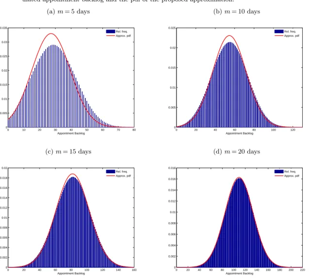
In order to asses the accuracy of the diffusion approximation, we compare a simulated backlog of appointments with the approximated one. For our simulation experiments we assume uniform patience, i.e. F∼U[0,2], and Poisson arrivals, i.e. G∼Exp(1). In Figure 3 we demonstrate such a comparison for a medical practice where λ= 33 appointment requests per day, s= 30 offered appointments per day, and for different patience levels. Our simulation experiments confirm that for moderately large values of m the proposed probability distribution is very accurate.
Figure 3 The distribution of the appointment backlog: a comparison between the frequency histogram of a sim-ulated appointment backlog and the pdf of the proposed approximation.
(a)m= 5 days 0 10 20 30 40 50 60 70 80 0 0.005 0.01 0.015 0.02 0.025 0.03 0.035 Appointment Backlog Rel. freq. Approx. pdf (b)m= 10 days 0 20 40 60 80 100 120 0 0.005 0.01 0.015 0.02 0.025 Appointment Backlog Rel. freq. Approx. pdf (c)m= 15 days 0 20 40 60 80 100 120 140 160 0 0.002 0.004 0.006 0.008 0.01 0.012 0.014 0.016 0.018 0.02 Appointment Backlog Rel. freq. Approx. pdf (d)m= 20 days 0 20 40 60 80 100 120 140 160 180 200 220 0 0.002 0.004 0.006 0.008 0.01 0.012 0.014 0.016 0.018 Appointment Backlog Rel. freq. Approx. pdf
Our next experiment concerns the effective arrival rate, the rate at which patients are assigned to appointment slots. In Table 1 we compare λeff from (14) with the actual effective arrival of
a simulated appointment book, for a range of traffic intensities. Our results suggest that, for moderately large patience, λeff approximates the effective arrival well, and
λeff≈min(λ, s). (15)
Table 1 Effective arrival rates forλ= 50 and different values ofsandm.
m s= 40 s= 45 s= 50 s= 55 s= 60
(days) λeff λsimeff λeff λsimeff λeff λsimeff λeff λsimeff λeff λsimeff 2 40.00 39.82 44.82 42.92 48.01 44.42 49.14 45.13 49.52 45.56 4 40.00 40.00 44.98 44.71 48.59 47.04 49.52 47.68 49.75 47.95 6 40.00 40.00 45.00 44.96 48.85 47.95 49.66 48.55 49.83 48.75 8 40.00 40.00 45.00 45.00 49.00 48.42 49.74 49.01 49.87 49.17 10 40.00 40.00 45.00 45.01 49.11 48.72 49.79 49.29 49.90 49.42 12 40.00 40.00 45.00 45.01 49.19 48.93 49.82 49.48 49.91 49.59 14 40.00 40.00 45.00 45.01 49.25 49.08 49.85 49.61 49.93 49.71 16 40.00 40.00 45.00 45.01 49.29 49.20 49.87 49.72 49.94 49.81 18 40.00 40.01 45.00 45.01 49.34 49.28 49.88 49.80 49.94 49.88 20 40.00 40.01 45.00 45.01 49.38 49.36 49.89 49.87 49.95 49.94
5. The In-Clinic Queue
In this section we study the in-clinic queue in order to characterize the patients’ waiting times and physicians’ overtime. The evolution of the queue highly depends on how the patients are scheduled to arrive throughout the working day, on patient’s no-show behavior and punctuality, and on the distribution of the service times as well. As discussed in§2, there are no analytical expressions for the patients’ waits and physicians’ overtime in the literature. Only under certain assumptions on the service times distribution (deterministic or exponential), and by assuming punctual patients, recursive expressions can be derived.
We model the in-clinic queue as aGI/GI/1 queue. The length of a regular working day isT hours, during which the offered appointments are allocated. Patients do not show up for their scheduled appointment with proobability 1−p∈[0,1). On a particular day, if ˆs patients are scheduled to see a physician, then the arrival rate to the clinic is λc=
pˆs
T patients per hour. The queue starts
empty at the beginning of the working day and the server continues to work during overtime as well, beyondT, until the queue empties.
5.1. Diffusion Approximation
For the arrival process we consider a sequence of iid random variables{uc,i:i≥0}, with associated
renewal processes Nc(t) = max{k≥0 : ∑k
i=1uc,i≤t}. The random variableuc,i denotes the
inter-arrival time between thei−1th andith patients with scheduled appointments, has finite meanλ−1 c
and finite squared coefficient of variationc2
For the service times we consider an independent sequence of iid random variables {vi:i≥0},
where vi corresponds to the service time of the ith arrival, has finite mean µ−1 and finite squared
coefficient of variationc2 v.
The workload right before theitharrival, denoted asW
i, can be expressed by the classical Lindley
recursion as
Wi= max{Wi−1+vi−1−uc,i,0}, fori≥2, (16)
andW1= 0.
As in Chen and Yao (2001) p. 142-144, the workload at time t, denoted asW(t), can be approx-imated asW(t)≈d 1
µY(t), where Y(t) is a regulated Brownian motion (RBM) with initial position Y(0) = 0, drift
α:=λc−µ, (17)
and infinitesimal variance
β2:=λcc 2
u+ min(λc, µ)c 2
v, (18)
reflected at zero. One representation ofY(t) is
Y(t) =X(t) +L(t), (19)
where L(t) = sup
0≤s≤t
[−X(t)] and X(t) =αt+βB(t),
with B(t) being a standard Brownian Motion. The representation of Y(t) in (19) is referred to as theSkorokhod representation. The pdf of Y(t), as given by Harrison (1985), is
fY(t)(x) =β2√tϕ(xβ−√αtt)−2αβ2e
2αx
β2 Φ(−x−αt
β√t ), x≥0. (20)
The aggregate in-clinic waiting time in the GI/GI/1 queue for the time interval [0, T] is
∑Nc(T)
i=1 Wi, and can be approximated as N∑c(T) i=1 Wi= ∫ T 0 W(t)dNc(t) = ∫ T n 0 nW(nt)dNc(nt) n d ≈ ∫ T n 0
nW(nt)dλct (for large nand from FSLLN)
=λc ∫ T 0 W(t)dt d ≈α+µ µ ∫ T 0 Y(t)dt=:Wc. (21)
The physician’s overtime is equal to W(T), the workload at the end of the regular working day, and is approximated as
Oc:= 1
µY(T). (22)
In what follows, we derive explicit expressions for E[Wc] andE[Oc]. Lemma 2. Assume that β2>0. Then E[∫0TY(t)dt] =
{
E[Y2(T)]−β2T
2α ifα̸= 0
E[Y3(T)]
3β2 ifα= 0.
The first two moments of an RBM with negative drift are derived in Abate and Whitt (1987) through Laplace transforms. The same methodology does not go through in the case of positive drift. As argued in the literature of reflected diffusions (see for example p. 144 of Chen and Yao (2001) or p. 184 of Whitt (2002)), when the drift is positive and for large t, the effect of reflection becomes negligible, and therefore an RBM is approximated with a BM. However, since clinics typically serve patients for a finite time interval [0, T] in the order of 8-12 hours, we need to include the reflection in our analysis, even for the case of positive drift when λc> µ.
Lemma 3. The first two moments of Y(t) are as follows:
E[Y(t)] = 0 if β= 0, α≤0 αT if β= 0, α >0 β√tϕ(α√t β ) + (αt+ β2 α)Φ( α√t β )− β2 2α if β >0, α̸= 0 2√β√t 2π if β >0, α= 0. E[Y2(t)] = 0 ifβ= 0, α≤0 α2T2 ifβ= 0, α >0 (βαt√t+β3√t α )ϕ( α√t β ) + (2β 2t+α2t2−β4 α2)Φ( α√t β ) + β4 2α2 ifβ >0, α̸= 0 β2t ifβ >0, α= 0.
Lemma 4. E[Y(t)] and E[Y2(t)]are continuous in α at α= 0.
Note that our proof of Lemma 3 provides an alternative proof for Theorem 1.1 of Abate and Whitt (1987), whereα=−1 andβ= 1. Now we can express the performance measures of interest as follows. Theorem 2. E[Oc] = 0 if β= 0, α≤0 αT µ if β= 0, α >0 1 µ[β √ T ϕ(α√T β ) + (αT+ β2 α)Φ( α√T β )− β2 2α] if β >0, α̸= 0 2β√T √ 2πµ if β >0, α= 0. E[Wc] = 0 ifβ= 0, α≤0 αT2(α+µ) 2µ ifβ= 0, α >0 α+µ 2µα3[(βα 3T√T+β3α√T)ϕ(α√T β ) + (2β 2α2T+α4T2−β4)Φ(α√T β ) + β4 2 −β 2α2T] ifβ >0, α̸= 0 4βT√T 3√2π ifβ >0, α= 0.
Our diffusion approximation for the in-clinic queue in transient state is tractable, and pro-vides explicit expressions for the performance measures of interest. It also captures patients’ non-punctuality and no-shows (for positivec2
u), and random service times (for positive c 2 v).
5.2. Simulation Experiments
Empirical studies suggest that the service times for certain medical practices have a lognormal distribution. Cayirli et al. (2006) analyze data collected from a primary health care clinic in a New York metropolitan hospital that provides service to about 300,000 outpatients a year. They find that a lognormal distribution with meanµ−1= 15.5 minutes and a coefficient of variationc
v= 0.325
is the best fit for the service times of return patients.
The Brownian approximation turns out to be very accurate, as demonstrated by our simulation experiments, under both light and heavy traffic. In Figure 4 we compare the expressions ofE[Wc]
and E[Oc] in Theorem 2, with the corresponding performance measures of a simulated clinic, for
different traffic intensities and for different levels of service times’ variability. For low values of the
cv (less than 0.5) our approximation performs very well, and, as variability increases, we tend to
slightly overestimate the aggregate waiting time and physician’s overtime.
5.3. An Extension to Account for Walk-Ins
The analysis in §5.1 can be extended to account for walk-ins. Consider a ∑2i=1GIi/GI/1 queue,
where the two streams of arrivals come from scheduled appointments and emergency walk-ins. Besides the model primitives in §5.1, consider further an independent sequence of iid random variables {uw,i:i≥0}, with associated renewal processesNw(t) = max{k≥0 :
∑k
i=1uw,i≤t}. The
random variable uw,i denotes the inter-arrival time between the i−1th and ith emergency
walk-in patients, has finite mean λ−1
w and finite squared coefficient of variation c 2
w. As a convention, uw,0= 0. The arrival process at the single server queue is a superposition of the two arrival streams {N(t) :=Nc(t) +Nw(t), t≥0}, with associated arrival times tn:= inf{t≥0 :N(t)≥n} and
inter-arrival timesτn:=tn−tn−1. The superposition arrival process{N(t), t≥0}is a renewal process if
and only if the processes{Nc(t), t≥0}and{Nw(t), t≥0}are Poisson. In Whitt (1982),{N(t), t≥0}
is approximated by a renewal process with the inter-arrival times having mean (λc+λw)−1 and
squared coefficient of variation λcc2u+λwc2w (λc+λw) .
Under this setting, the patients’ expected aggregate waiting time and physician’s overtime can be approximated as in Theorem 2, with the drift αbeing replaced with ˆα:=λc+λw−µ, and the
infinitesimal varianceβ2 being replaced with ˆβ2:=λ
cc2u+λwc2w+ min(λc+λw, µ)c2v. For the rest of
Figure 4 Physician’s overtime and aggregate waiting time: a comparison between the diffusion approximation and a simulated clinic.
(a)µ∈ {2,3,4}, 0≤λc≤3,cv= 0.325. 0 0.5 1 1.5 2 2.5 3 0 10 20 30 40 50 60 70 λc µ= 2 - simul. µ= 2 - approx. µ= 3 - simul. µ= 3 - approx. µ= 4 - simul. µ= 4 - approx. E[Wc] (b)µ= 4,λc∈ {3,4,5}, 0≤cv≤1. 0 0.1 0.2 0.3 0.4 0.5 0.6 0.7 0.8 0.9 1 0 10 20 30 40 50 60 70 80 cv λc= 3 - simul. λc= 3 - approx. λc= 4 - simul. λc= 4 - approx. λc= 5 - simul. λc= 5 - approx. E[Wc] (c)µ∈ {2,3,4}, 0≤λc≤3,cv= 0.325. 0 0.5 1 1.5 2 2.5 3 0 1 2 3 4 5 λc µ= 2 - simul. µ= 2 - approx. µ= 3 - simul. µ= 3 - approx. µ= 4 - simul. µ= 4 - approx. E[Oc] (d)µ= 4,λc∈ {3,4,5}, 0≤cv≤1. 0 0.1 0.2 0.3 0.4 0.5 0.6 0.7 0.8 0.9 1 0 0.5 1 1.5 2 2.5 3 cv λc= 3 - simul. λc= 3 - approx. λc= 4 - simul. λc= 4 - approx. λc= 5 - simul. λc= 5 - approx. E[Oc]
Note. The arrival process is Poisson, the service times are Lognormal with mean µ−1 hours and standard deviation
cv×µ−1,T= 8 hours.
6. Optimal Panel Sizing and Appointment Scheduling
Having developed the necessary tools to approximate the appointment backlog and the in-clinic queue, we aim to maximize the long run average daily net benefit of the medical facility from providing care to patients with respect to the panel size,N, and the number of offered appointment slots per working day,s. We assume thatλis strictly increasing inN, and therefore it is equivalent to perform the optimization with respect toλand s.
As a reminder, we consider a reward r >0 generated per patient served, a holding cost ca>0
for each day that each patient who joins the backlog has to wait for her scheduled appointment, a waiting cost cw>0 per hour that each patient has to wait in the clinic to see the physician, and
an overtime cost co>0 per hour.
Recall that the analysis of the in clinic queue in §5 is based on a fixed arrival rate for a given day. For an arbitrary day,λc is a random variable governed by the distribution of the appointment
backlog in (11), and depends on the no-show probability.
We approximate the average daily net benefit of the medical facility from providing care to patients in (1) as R(λ, s) : =rpλeff−caλeffE[W a ]−cwEλc[E[W c ]]−coEλc[E[O c ]] =rpλeff−caE[Qa]−cwEλc[E[W c]]−c oEλc[E[O c]], (23)
where E[Qa] is as in (12), and E[Wc] and E[Oc] are as in Theorem 2, with α=λ
c−µ and
β2=λ
cc2u+ min(λc, µ)c2v. We consider the optimization problem
max
λ,s R(λ, s)
s.t. λ, s≤M λ, s≥0.
(P)
The constraintλ, s≤M ensures that demand and supply for appointments cannot be arbitrarily large. Lemmas 1(a) and 5, and Weierstrass’ extreme value theorem guarantee the existence of an optimal solution to (P).
6.1. Characterization of the Optimal Solution
The optimization problem (P) is analytically intractable; the objective function involves the pdf, cdf, and hazard rate of a standard Normal random variable. However, if we make one simplifying assumption, motivated by (15) and for the sake of tractability, we are able to provide a neat characterization of the optimal solution.
Theorem 3. Assume thatλc=
pmin(λ,s)
T with probability one, and let(λ
∗, s∗)be an optimal solution
to (P). Then λ∗≤s∗ and the following three cases are exhaustive: (a) λ∗= 0 and ∂R∂λ|(0,s∗)≤0.
(b) 0< λ∗≤s∗=M. (c) 0< λ∗=s∗<4m(πF′(0)θ−22)π2.
Under the assumptions of Theorem 3, supply for medical appointments should be at least as high as the demand in outpatient care, and furthermore, (P) reduces to a single variable optimization problem. The optimal solution to the panel sizing and scheduling problem lies within one of the following three regimes. Either:
(a) It is not beneficial for the clinic to maintain a panel of patients and schedule appointments at all, or
(b) The clinic offers as many appointment slots as possible, and the optimal daily demand for medical appointments depends on the objective function’s coefficients and the clinic’s charac-teristics, or
(c) Supply and demand are perfectly matched and are very small.
In our extensive numerical experiments the optimal pair (λ∗, s∗) almost always lies within regime (b), which we refer to as the “Open Access” regime, since the clinic offers as many appointment slots as possible. One scenario that yields a solution in regime (c), which we refer to as the “Limited Access” regime, is when the average service time is large, and the patients are very sensitive to the appointment delay. In practice, such a scenario could correspond to a clinic that performs long, complex, urgent procedures.
Throughout our numerical/simulation experiments, we normalize the objective function with respect to cw, i.e., cw= 1. Following Robinson and Chen (2010), we consider an overtime cost
coefficient which is five times as much as the patients’ waiting cost coefficient, i.e.,co= 5. Further,
we regard that the cost of waiting one day for an appointment is in the same order as the cost of waiting one hour in the clinic, i.e., ca∼cw. Finally, the average reward generated per hour is in
the same order as the cost of staying one hour overtime in the clinic, i.e.,rµ∼co.
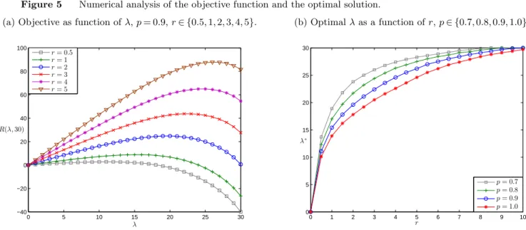
For fixed s, the objective function appears to be concave in λ on [0, s] as demonstrated by our numerical analysis. This suggests that a first order condition would uniquely determine the approximated global maximum. Figure 5(a) demonstrates the behavior of the objective function with respect toλfor different values ofr, while the cost coefficients are kept constant. Figure 5(b) demonstrates the optimal solution as given by the MATLAB R2012b optimization toolbox. It is evident that the no-show probability has a significant, non-linear effect on the panel sizing decision and should be taken under consideration. Further, asr increases, with values greater than co
µ, the
arrival rate increases in a concave manner towards heavy traffic, i.e.,λ→s. For reasonable values of
r, the system operates in light traffic, and hence an Open Access policy (satisfying today’s demand today) is evidently optimal.
6.2. A Simulation Experiment
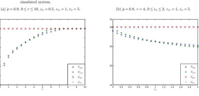
In order to characterize the optimal solution in Theorem 3, we assumed that the arrival rate to the clinic from scheduled appointments is the same every day and equal is top×min(λ, s) patients per day. In Figure 6 we compare the optimal pair (λ, s) for a simulated system with the one obtained under the assumptions of Theorem 3, for different cost/reward coefficients. Our experimental setup is as follows:
Figure 5 Numerical analysis of the objective function and the optimal solution. (a) Objective as function ofλ,p= 0.9,r∈ {0.5,1,2,3,4,5}.
0 5 10 15 20 25 30 −40 −20 0 20 40 60 80 100 λ r= 0.5 r= 1 r= 2 r= 3 r= 4 r= 5 R(λ,30) (b) Optimalλas a function ofr,p∈ {0.7,0.8,0.9,1.0}. 0 1 2 3 4 5 6 7 8 9 10 0 5 10 15 20 25 30 r p= 0.7 p= 0.8 p= 0.9 p= 1.0 λ∗
Note. The objective function appears to be concave in λon [0, s], as suggested by our numerical experiments. For this example:s∗=M= 30, the balking threshold is uniformly distributed between 0 and 10 days, the arrivals to the appointment book and the clinic are Poisson,T= 8 hours, ca=cw=15co= 1,µ= 3 patients per hour (24 patients per day),cv= 0.325.
• Appointment book: Requests for appointment arrive according to a Poisson process at a rate λper day, and sappointment slots are offered per day. There is an upper bound M= 30 for both λand s. The balking threshold is uniformly distributed with an average ofm= 5 days.
• Clinic:The length of the working day isT= 8 hours. Depending on the state of the appoint-ment book at the beginning of dayk,λk patients are scheduled to arrive, 1≤k≤10000. There is a
no-show rate 1−p. As argued earlier in this paper, the arrival process depends on how the patients are scheduled to arrive throughout the working day and on their punctuality. For our experimental setup, we consider a Poisson arrival process from scheduled appointments with rate pλk
T per hour.
Finally, the service times are iid, lognormally distributed with mean 20 minutes and coefficient of variation 0.325.
We observe that indeed the optimal solution lies within the Open Access regime for both systems, and further, our approximated solution to the panel sizing decision is close to the one that optimizes the simulated system.
7. Conclusion
We study the joint problem of determining the panel size of a medical practice and the number of offered appointments per day, so that patients do not face long backlogs, and the medical facility is not overcrowded. We explicitly model the two separate time scales involved in accessing medi-cal care: appointment delay (order of days, weeks) and clinic delay (order of minutes, hours). We
Figure 6 Simulation Study: A comparison between the approximated solution and the one that optimizes a simulated system. (a)p= 0.9, 0≤r≤10,ca= 0.5,cw= 1,co= 5. 0 1 2 3 4 5 6 7 8 9 10 0 5 10 15 20 25 30 35 r λ∗ app λ∗ sim s∗ app s∗ sim (b)p= 0.8,r= 4, 0≤ca≤2,cw= 1,co= 5. 0 0.2 0.4 0.6 0.8 1 1.2 1.4 1.6 1.8 2 15 20 25 30 32 ca λ∗ app λ∗ sim s∗ app s∗ sim
analyze the two queueing systems associated with each type of delay, and provide explicit expres-sions for the performance measures of interest based on diffusion approximations. In our analysis we capture many features of the complex reality of the healthcare system, including patients’ non-punctuality, no-shows, and stochastic service times. Two additional distinctive characteristics of this study are the balking behavior of the patients who face long appointment backlogs, and the transient-state analysis of the in-clinic queue, which allow the study of a system with traffic intensity greater than one and bear unique technical challenges.
Concerning the panel sizing and appointment scheduling decisions, our analysis provides theoret-ical and numertheoret-ical support that either an “Open Access” policy is optimal, or supply and demand are perfectly matched and are both very small (“Limited Access” regime). Under our Open Access regime, the clinic offers as many appointment slots as possible per day, and the optimal panel size depends on the cost structure and the clinic’s characteristics. A solution within the Limited Access regime arises when the service times are long, and the patients are very sensitive to the appointment delay.
There are a few research directions that we further intend to explore. In this study, the no-show rate is treated as constant, and does not depend on the appointment backlog. Empirical studies though suggest that the probability of a patient not showing up depends on the appointment delay (Gallucci et al. (2005), Dreiher et al. (2008), Norris et al. (2012)). Letγ(k) denote the probability of a patient who faces an appointment backlog ofkpatients being a no-show, increasing ink. One expression forγ(k) is given in Green and Savin (2008):γ(k) =γmax−(γmax−γmin)e−⌊
k s⌋C−
1
γmax and γmin are the maximum and minimum observed no-show rates respectively, and C is a
constant that captures the characteristics of the medical practice.
We have assumed that patients arrive at the clinic according to a renewal process. The literature of appointment scheduling under no-shows suggests that a front loaded schedule is optimal, i.e., more patients are scheduled to arrive towards the beginning of the working day (see for example Robinson and Chen (2010), LaGanga and Lawrence (2012), Zacharias and Pinedo (2013)). Such a clinic withfront loadedschedules can be approximated as follows: the working day is partitioned in two time intervals [0, T1]∪(T1, T] = [0, T], with the first interval having a higher arrival rate than
the second one. Then, the workload can be approximated accordingly by a reflected diffusion with a piecewise constant drift, and a piecewise constant infinitesimal variance. Further, it is of interest to analyze a system with a more refined arrival process, where patients who show up arrive at the time of their scheduled appointment plus a stochastic noise.
A careful treatment of the emergency walk-ins is of interest as well. As demonstrated in§5.3, the analysis of the in-clinic queue can be readily adjusted to capture emergency walk-ins, given that we know their arrival rate. A relationship should be established first between the walk-in rate, and the state of the appointment backlog and the clinic’s panel size.
Finally, our closed-form expressions for the expected patients’ in-clinic waiting time and physi-cian’s overtime can be used effectively to make scheduling decisions dynamically. An optimal appointment assignment rule may be developed for incoming requests, based on the state of the appointment book, and in anticipation of future demand. Such a dynamic scheduling setting can also capture a seasonal effect (for example flu) on the demand for medical care.
Appendix. Proofs
Proof of Theorem 1 As in Ward and Glynn (2005), we represent the appointment backlog in terms of the martingale{(M(i),Fi) :i≥0}, whereFi=σ((u1, w1), ...,(ui, wi), ui+1)⊂ F, and
M(i) : = i ∑ j=1 [ 1{Q(t − j) s ≥mwj} −E ( 1{Q(t − j) s ≥mwj}|Fj−1 )] = i ∑ j=1 [ 1{Q(t − j) s ≥mwj} −F ( Q(t−j) sm )] . (24)
We can now write the evolution equation for the backlog as a stochastic integral
Q(t) + ∫ t 0 F ( Q(τ−) ms ) dA(τ) =A(t)−M(A(t))−s⌊t⌋+L(t). (25)
Consider further the diffusion scaled process ˜Mn(t) := Mn(⌊nt⌋)
√n . From the pathwise equation for the backlog of appointments in (25), Assumption 1, the scaling in (3) and (4), and some algebra, we obtain ˜ Qn(t) +sF′(0) ∫ t 0 ˜ Qn(τ)dτ= ˜Xn(t) + ˜Ln(t), (26) where ˜ Xn(t) = ˜An(t) +√1 n(nλnt−s⌊nt⌋)−M˜ n ( ¯An(t)) +sF′(0) ∫ t 0 ˜ Qn(τ)dτ− ∫ t 0 √ nF(Q˜√n(τ)n )dA¯n(τ). (27) To provide an intuition for the representation of the workload in (26), note that from L’Hˆospital’s rule lim y→∞yF( x y) =F ′(0)x, so that 1 √n ∫ nt 0 F(Q(τ)ms )dA(τ) = ∫ t 0 √ nF(Q˜√n(τ)n )dA¯n(τ)≈d ∫ t 0 sF′(0) ˜Qn(τ)dτ (from(29)).
Note that ˜Ln(0) = 0, ˜Ln is non-decreasing, ˜Ln increases only when ˜Qn= 0. Therefore for γ= sF′(0) we have ( ˜Qn,L˜n) = (Φ
γ,Ψγ)( ˜Xn).
Next, we wish to derive a diffusion limit for the process ˜Xn(t). Under Assumption 1, and from
theFunctional Central Limit Theorem and Functional Strong Law of Large Numbers, ˜ An(t)⇒√sθB(t), (28) ¯ An(t)→st, (29) and √1 n(nλnt−s⌊nt⌋)→ηt, (30)
where B(t) is a standard Brownian motion. Ward and Glynn (2005) proved (in their Theorem 1) that ˜ Mn( ¯An(t))⇒0 (31) and ∫ t 0 sF′(0) ˜Qn(τ)dτ− ∫ t 0 √ nF(Q˜√n(τ) n )dA¯ n (τ)⇒0. (32)
Combining (27), (28), (29), (30), (31), (32) we get the desired weak convergence for ˜Xn(t)
˜
Xn(t)⇒√sθB(t) +ηt.
From the continuity of the Linearly Generalized Regulator Mapping, and from the Continuous Mapping Theorem, we finally conclude that
( ˜Qn(t),L˜n(t))⇒(Φγ,Ψγ)( √
sθB(t) +ηt),
Proof of Lemma 1 (a) Suppose that m, s >0. Firstly we show that lim λ→0E[Q a] = 0. lim λ→0E[Q a ] = lim λ→0 [ ms(λ−s) λF′(0) + √ msθ2 2F′(0)h ( s−λ λ √ 2ms F′(0)θ2 )] = lim λ→0 [ ms(λ−s) λF′(0) + √ msθ2 2F′(0) ϕ ( λ−s λ √ 2ms F′(0)θ2 ) Φ ( λ−s λ √ 2ms F′(0)θ2 ) ] = lim λ→0 [ ms(λ−s) λF′(0) + √ msθ2 2F′(0) −λs2 2ms F′(0)θ2 λ−s λ ϕ ( λ−s λ √ 2ms F′(0)θ2 ) s λ2 √ 2ms F′(0)θ2ϕ ( λ−s λ √ 2ms F′(0)θ2 ) ] (33) = lim λ→0 [ ms(λ−s) λF′(0) − √ msθ2 2F′(0) √ 2ms F′(0)θ2 λ−s λ ] = 0,
where (33) comes from the fact that lim
λ→0ϕ ( λ−s λ √ 2ms F′(0)θ2 ) = lim λ→0Φ ( λ−s λ √ 2ms F′(0)θ2 ) = 0 and L’Hˆospital’s rule.
Then we show that lim
λ→0 ∂E[Qa]
∂λ = 0. It is well known that limx→∞h′(x) = 1 (see for example Barrow
and Cohen (1954)), and therefore lim λ→0 ∂E[Qa] ∂λ = limλ→0 [ ms F′(0) s λ2− √ msθ2 2F′(0) s λ2 √ 2ms F′(0)θ2h′ ( s−λ λ √ 2ms F′(0)θ2 )] = lim λ→0 [ ms F′(0) s λ2− ms F′(0) s λ2 ] = 0.
(b) Suppose thatλ, m, s >0. ThenE[Qa] = √ msθ2 2F′(0)[h(y)−y], wherey:= √ 2ms F′(0)θ2 (s−λ) λ . Therefore ∂E(Qa) ∂λ = √ msθ2 2F′(0) ∂y ∂λ[h ′(y)−1] =− √ msθ2 2F′(0) √ 2ms F′(0)θ2 s λ2[h′(y)−1] = ms2 F′(0)λ2[1−h′(y)].
It is well known that 0< h′(x)<1 for all x∈R (see for example Barrow and Cohen (1954)), concluding that ∂E[Q∂λa]>0 for λ >0.
(c) Suppose thatλ, m, s >0. ThenE[Qa] = √ msθ2 2F′(0)[h(y)−y], wherey:= √ 2ms F′(0)θ2 (s−λ) λ . Therefore ∂E(Qa) ∂m = 1 2√m √ sθ2 2F′(0)[h(y)−y] + √ msθ2 2F′(0) ∂y ∂m[h ′(y)−1]. (34)
From (34) and some algebra, the condition ∂E[Q∂ma] >0 is true if and only ifh(y)−2y+yh2(y)− y2h(y)>0. From Theorem 2.5 of Baricz (2008), the functionx7→xh(x)[ 1
h(x) ]′ is strictly decreasing on (0,∞), implying that [ xh(x) [ 1 h(x) ]′]′ <0
⇐⇒[xh(x)−hh2′(x)(x) ]′ <0 ⇐⇒[xh′(x) h(x) ]′ >0 (35) ⇐⇒xh′′(x)+h′(x)h(x)−x[h′(x)]2 h2(x) >0 ⇐⇒xh2(x)[h(x)−x]2+xh3(x)[h(x)−x]−xh2(x)+h2(x)[h(x)−x]−xh2(x)[h(x)−x]2 h2(x) >0 (36) ⇐⇒h2(x)[h(x)−2x+xh2(x)−x2h(x)] h2(x) >0 ⇐⇒h(x)−2x+xh2(x)−x2h(x)>0, forx >0, (37) where (35) follows from the fact theh(x)>0 for all x∈R, and (36) follows from:
h′(x) =h(x)[h(x)−x] (38) and h′′(x) =h(x)[h(x)−x]2+h2(x)[h(x)−x]−h(x). (39) (d) For fixed λ, m >0, it suffices to show that every critical point of E[Qa] (with respect to s)
is a local maximum, i.e., ∂2E[Q∂s2a] <0 whenever
∂E[Qa]
∂s = 0. Then, since E[Q
a] is continuous (and
differentiable) in s, there can be at most one local maximum, concluding that E[Qa] is unimodal
ins. Firstly, we prove the following intermediate result:
Lemma 6. Let h(x) := 1−ϕ(x)Φ(x) be the hazard rate of a standard Normal random variable. Then h′′(x)[h(x)−x] [h′(x)−1]2 <2 for all x∈R. Proof of Lemma 6 h′′(x)[h(x)−x] [h′(x)−1]2 <2 ⇐⇒h(x)[h(x)−x]3+h2(x)[h(x)−x]2−h(x)[h(x)−x] 1−2h(x)[h(x)−x] +h2(x)[h(x)−x]2 <2 (40) ⇐⇒0<−h(x)[h(x)−x]3+h2(x)[h(x)−x]2−3h(x)[h(x)−x] + 2, (41) where (40) follows from (38) and (39). Barrow and Cohen (1954) proved that inequality (41) holds.
Recall that for λ, s >0
E[Qa] = √ mθ2 2F′(0) √ s[h(y)−y], (42) wherey:= √ 2m F′(0)θ2 √s(s−λ) λ . (43) Then ∂y ∂s = √ 2m F′(0)θ2 ( 3√s 2λ − 1 2√s ) =3y2s+√1 s √ 2m F′(0)θ2, (44) ∂2y ∂s2 = 3 2s ∂y ∂s− 3y 2s2− 1 2s√s √ 2m F′(0)θ2, (45) and ∂E[Q∂sa]= √ mθ2 2F′(0) [ 1 2√s[h(y)−y]− √ s[1−h′(y)]∂y∂s ] . (46)
![Figure 2 E[Q a ] is increasing in λ and m, and unimodal in s.](https://thumb-us.123doks.com/thumbv2/123dok_us/532579.2562795/10.892.86.827.137.846/figure-e-q-increasing-λ-m-unimodal-s.webp)