Urban Pluvial Flood Forecasting

by

Nuno Eduardo da Cruz Simões

A thesis submitted for the degree of Doctor of Philosophy and for the Diploma of the Imperial College London

Declaration

The work presented in this thesis is my own except where otherwise acknowl-edged.

Two main approaches to enhance urban pluvial ood prediction were developed and tested in this research: (1) short-term rainfall forecast based on rain gauge networks, and (2) customisation of urban drainage models to improve hydraulic simulation speed. Rain gauges and level gauges were installed in the Coimbra (Portugal) and Redbridge (UK) catchment areas. The collected data was used to test and validate the approaches developed.

When radar data is not available urban pluvial ooding forecasting can be based on networks of rain gauges. Improvements were made in the Support Vector Machine (SVM) technique to extrapolate rainfall time series. These improve-ments are: enhancing SVM prediction using Singular Spectrum Analysis (SSA) for pre-processing data; combining SSA and SVM with a statistical analysis that gives stochastic results. A method that integrates the SVM and Cascade-based downscaling techniques was also developed to carry out high-resolution (5-min) precipitation forecasting with longer lead time. Tests carried out with histor-ical data showed that the new stochastic approach was useful for estimating the level of condence of the rainfall forecast. The integration of the cascade method demonstrates the possibility of generating high-resolution rainfall forecasts with longer lead time. Tests carried out with the collected data showed that water level in sewers can be predicted: 30 minutes in advance (in Coimbra), and 45 minutes in advance (in Redbridge).

A method for simplifying 1D1D networks is presented that increases computa-tional speed while maintaining good accuracy. A new hybrid model concept was developed which combines 1D1D and 1D2D approaches in the same model to achieve a balance between runtime and accuracy. While the 1D2D model runs in about 45 minutes in Redbridge, the 1D1D and the hybrid models both run in less than 5 minutes, making this new model suitable for ood forecasting.

Acknowledgements

I wish to express my gratitude to:

The Portuguese Science and Technology Foundation (SFRH/BD/37797/2007) by their nancial support.

The Department of Civil Engineering, University of Coimbra for the giving me the opportunity to enrol in this PhD programme.

My supervisors, Professor ƒedo Maksimovi¢ and Professor Alfeu Sá Marques for their guidance, invaluable knowledge and for providing me with the opportunity to carry out this research.

Dr Onof for his advices about the rainfall subjects of this research.

Professor Lopes de Almeida for let me install the raingauge in his house, to Escola Secundária José Falcão and Department of Mathematics of University of Coimbra for the permission to install raingauges on their roof.

Professor Gil Goncalves for providing me the DTM of Coimbra.

Mr Joaquim Cordeiro for helping me with his assistance and ideas to install all the equipment in Coimbra.

AC, Águas de Coimbra, EMM for their assistance during installations and data collection in Coimbra.

My friends and colleagues João Leitão, Lipen Wang, Susana Ochoa and Rui Pina for their invaluable assistance during this work.

My colleagues from Imperial College London and University of Coimbra who helped me in many ways.

My friend José Pedro for the good times and support in London.

À Andreia e à Alice pela cumplicidade constante, estímulo, apoio e paciência perante a minha ausência. Aos meus pais pelo encorajamento e ajuda. À minha família pelo incentivo, aos meus sogros e cunhada pelo apoio.

1D 1D1D 1D2D 2D AOFD ci DEM DSM DTM EA FRMRC fst GIS LiDAR NWP SSA SSA+SVM Stoc SSA Stoc SVM SVM TIN UKWIR UWRG One-dimensional

Dual drainage model (1D sewer and 1D overland network) Dual drainage model (1D sewer and 2D overland network) Two-dimensional

Automatic Overland Flow Delineation characteristic curve i

Digital Elevation Model Digital Surface Model Digital Terrain Model UK Environmental Agency

Flood Risk Research Management Consortium Forecasting Start Time

Geographic Information Systems Light Detection And Range Numerical Weather Prediction Singular Spectrum Analysis

SVMachine with SSA pre-processing Stochastic Singular Spectrum Analysis Stochastic Support Vector Machine Support Vector Machine

Triangulated Irregular Network UK Water Industry Research

Contents

1 Introduction 16

1.1 Context . . . 16

1.2 Aims and objectives . . . 18

1.3 Methodology and originality of the work . . . 18

1.4 Thesis outline . . . 19

1.5 Case studies . . . 20

1.5.1 Zona Central catchment in Coimbra, Portugal . . . 20

1.5.2 Cranbrook catchment in the London Borough of Red-bridge, United Kingdom . . . 20

2 Literature Review 22 2.1 Urban pluvial ooding . . . 22

2.2 The impacts of urban pluvial ooding on society . . . 23

2.3 Rainfall data for urban drainage modelling . . . 25

2.3.1 Introduction . . . 25

2.3.2 Raingauges . . . 26

2.3.2.1 General characteristics of raingauges . . . 26

2.3.2.2 Interpolation techniques . . . 27

2.3.3 Weather radar . . . 31

2.3.4 Rainfall data requirements summary . . . 32

2.4 Modelling approaches in urban drainage . . . 32

2.4.2 Free surface ow equations . . . 34

2.4.2.1 Urban drainage models . . . 36

2.4.2.2 Existing Flood Models . . . 43

2.4.3 Automatic Overland Flow Delineation (AOFD) . . . 44

2.4.4 Summary of modelling approaches in urban drainage . . . 46

2.5 Flood Forecasting . . . 47

2.5.1 Rainfall Forecast . . . 48

2.5.1.1 Extrapolation in time techniques . . . 49

2.5.1.2 Quantitative Precipitation Forecast systems . . . 50

2.5.2 Linking QPF with hydrology . . . 51

2.5.3 Uncertainty and error propagation in ood forecasting . 53 2.5.4 Urban ood forecast systems . . . 54

2.5.5 Summary of ood forecasting . . . 54

2.6 Summary . . . 55

3 Case studies 56 3.1 Zona Central Catchment, Coimbra, Portugal . . . 56

3.1.1 Experimental setup . . . 57

3.1.1.1 Raingauges . . . 58

3.1.1.2 Levelgauges . . . 59

3.2 Cranbrook Catchment, London Borough of Redbridge, United Kingdom . . . 61

3.2.1 Experimental setup . . . 62

3.2.1.1 Raingauges . . . 63

3.2.1.2 Levelgauges . . . 64

3.3 Hydraulic Models . . . 65

4 Flood Forecasting based on raingauges networks 68 4.1 Context . . . 69

CONTENTS

4.2.1 Introduction . . . 70

4.2.2 Support Vector Machine (SVM) . . . 71

4.2.3 Singular Spectrum Analysis (SSA) . . . 74

4.2.4 Combined application of SVM and SSA: SSA + SVM . . 77

4.2.5 Stochastic SSA in synergy with SVM: Stoc SVM . . . 79

4.2.6 SVM enhanced with time series downscaling . . . 81

4.2.7 Results . . . 84

4.2.7.1 Rainfall data set . . . 84

4.2.7.2 Rainfall forecast . . . 85

4.2.7.3 Rainfall forecast enhanced with cascade method 92 4.3 Methodology for ood forecasting based on raingauge network . . 95

4.3.1 Interpolation technique and generation of rain-elds . . . 97

4.3.2 Application to Coimbra case study . . . 97

4.3.3 Application to London case study . . . 100

4.4 Conclusions . . . 103

5 Customisation of drainage networks 105 5.1 Introduction . . . 105

5.2 Dual drainage, 1D1D and 1D2D models . . . 106

5.3 1D1D simplied models . . . 108

5.3.1 Traditional simplication . . . 108

5.3.2 Two-step simplication . . . 110

5.3.3 Application of simplication techniques . . . 112

5.4 Hybrid models . . . 120

5.4.1 Advantages and disadvantages of 1D1D and 1D2D models 120 5.4.2 Hybrid model setup . . . 123

5.5 Hybrid model application . . . 127

5.5.1 Coimbra case study . . . 128

5.5.2 Redbridge case study . . . 131

6 Conclusions and further research 144 6.1 Overview . . . 144 6.2 Urban pluvial ood forecasting based on rain gauge networks . . 145 6.3 Customisation of drainage network models . . . 146 6.4 Further potential research . . . 147

6.4.1 Future work required in short term rainfall forecast based on raingauges networks . . . 147 6.4.2 Future work required in urban drainage modelling . . . . 148 6.4.3 Further work required in eld testing and calibration of

overland ow systems . . . 149 6.4.4 Further work required in urban pluvial ood forecasting . 149

References 150

A Calibration of hydraulic models 160

A.1 Calibration of Coimbra model . . . 160 A.2 Calibration of Cranbrook model . . . 164

List of Figures

1.1 Recent oods in Zona Central, Coimbra. . . 21 1.2 Recent oods in Cranbrook catchment, Redbridge. . . 21 2.1 Approximate ood hazard thresholds (Smith and Petley, 2009) . 24 2.2 Rainfall data resolution requirements (Einfalt, 2005) . . . 26 2.3 Overview of processes incorporated in a storm water model

(ad-apted from Zoppou (2001)). . . 33 2.4 Stages of sewer surcharge (Schmitt et al., 2004) . . . 37 2.5 Traditional approaches when water reaches the surface a) water

is lost b)water is stored and returns later to the system c) virtual reservoir (Wallingford Software 2009) . . . 37 2.6 Idealised surface and storm sewer ow components in dual

drain-age systems (Djordjevic et al., 1999). . . 39 2.7 Preissmann slot (Preissmann, 1961) . . . 40 2.8 Interactions between various stages in the modelling approach for

a ooded urban drainage system (Mark et al., 2004). . . 41 2.9 Conceptualisation of Integrated Urban Drainage Model Blanksby

et al. (2007) . . . 42 2.10 Storage cell procedure scheme (Bates, 2012) . . . 44 2.11 Types of surface pathways calculated from the DEM (Maksimovic

et al, 2009) . . . 45 2.12 Application of IC GIS-based tool to generate overland pathways.

3.1 Zona Central Catchment. The blue circle highlights the most

critical area. . . 57

3.2 Raingauges and levelgauges locations. . . 58

3.3 Raingauge, datalogger and PC connection interface . . . 59

3.4 Installed raingauges. . . 59

3.5 Solinst Junior levelgauge and connection to PC. . . 60

3.6 Levelgauge apparatus in sewer. . . 60

3.7 Levelgauge cable in the manhole cover for easy access. . . 61

3.8 Levelgauge in the surface . . . 61

3.9 River Roding Catchment . . . 62

3.10 Experimental Setup . . . 63

3.11 Raingauges . . . 64

3.12 Levelgauge sensors . . . 64

3.13 Open channel measurements . . . 65

3.14 DTM and sewer system . . . 65

3.15 Cranbrook network . . . 66

4.1 Diagram of time series prediction using SVR (Sato et al., 2008) . 73 4.2 Schematic of the sliding-window for time series prediction using SVM . . . 74

4.3 Rainfall data series, smoothed series and residuals. . . 75

4.4 Flowchart of the application of SVM and SSA . . . 78

4.5 Flowchart of the stochastic SSA in synergy with SVM . . . 79

4.6 Residuals series and characteristic curves. . . 81

4.7 Peak time prediction in Stochastic SVM technique . . . 81

4.8 Conceptual schematic of a cascade process, where a coarser volume in a specic scale is repeatedly subdivided into numbers of sub-volumes according to certain time-scale (set) and intensity (meas-ure) fragmentation ratios (S and W) (Wang et al., 2011). . . 83

4.9 Downscaling . . . 84

4.10 Eect of training sample number on forecasting. Left: 39 samples; middle: 51 samples; right: 986 samples. . . 85

LIST OF FIGURES 4.11 a) Rainfall events tested and b) Return period of selected rainfall

events . . . 86

4.12 Rainfall prediction of 31/01/1955 event with the dierent tech-niques . . . 87

4.13 Rainfall prediction of 23/05/2004 event with the dierent tech-niques . . . 88

4.14 Rainfall prediction of 09/04/1946 event with the dierent tech-niques . . . 89

4.15 Rainfall prediction of the 1st frequency using SVM (23/05/2004 event) . . . 90

4.16 Rainfall prediction of the 1st frequency using SVM (31/01/1955 event) . . . 90

4.17 Rainfall prediction of the 1st frequency using SVM (09/04/1946 event) . . . 90

4.18 a) Log-log plot of moment as a function of time-scale between 120 min and 5 min for 0.0≤q≤5.0; b) The observed and theoretical (log-Poisson) K(q) curves, respectively drawn by the grey dashed and the dark solid lines. . . 93

4.19 Example of 5 minutes observed data vs 15 minutes observed data (downscaled to 5 minutes) . . . 93

4.20 Rainfall prediction of 25-10-2006 event . . . 94

4.21 Rainfall forecast and generation of rain elds. . . 95

4.22 Flowchart of the methodology for ood forecasting based on raingauges networks . . . 96

4.23 Zona Central Catchment in Coimbra, Portugal. . . 98

4.24 Rainfall recorded in 3 raingauges on the 8/10/2010 event in Coim-bra . . . 98

4.25 Three consecutive rain-elds based on the forecast result of the 3 raingauges (forecast start time: 17h10min) and the resulting spatial interpolation for the 08/10/2010 event . . . 99

4.26 Rainfall recorded and predicted on the 08/10/2010 . . . 99

4.27 Water levels simulated and predicted at 8/10/2010 . . . 100

4.29 Rainfall recorded in 3 raingauges on the 14/01/2011 event . . . . 101

4.30 Three consecutive rain-elds based on 3 raingauges and spatial interpolation . . . 102

4.31 Recorded and forecasted rainfall on the 14-01-2011. . . 102

4.32 Water level simulated and predicted on the 14-01-2011 . . . 102

5.1 Example of the 1D1D model output . . . 107

5.2 Example of the 1D2D model output . . . 107

5.3 Simplication technique: Pruning: a) before pruning; b) after one pruning iteration (Haested Methods 2002) . . . 108

5.4 Simplication technique: Merging: a) before merging; b) after merging (Haested Methods, 2002) . . . 109

5.5 Sub catchment assigment using pruning technique . . . 109

5.6 Sub catchment assigment using merging technique . . . 110

5.7 Example of links between the sewer system and overland network (sewer network is represented in green and the overland network is represented in dark red). . . 111

5.8 Simplication procedures . . . 112

5.9 Vale das Flores catchment, Coimbra, Portugal . . . 113

5.10 1D sewer model (1D) of Vale das Flores catchment . . . 113

5.11 1D sewer model pruned (1Dp) of Vale das Flores catchment . . . 114

5.12 1D sewer model merged (1Dm) of of Vale das Flores catchment . 114 5.13 1D sewer model pruned and merged (1Dpm) of Vale das Flores catchment . . . 114

5.14 1D1D drainage networks of Vale das Flores catchment. Complete 1D1D model (1D1D) . . . 115

5.15 1D1D drainage networks of Vale das Flores catchment. 1D1D model pruned and merged together ((1D1D)pm) in red. Removed elements in black . . . 115

5.16 1D1D drainage networks of Vale das Flores catchment. Sewer sys-tem pruned and merged and complete overland model (1Dpm/1D) in green. Removed elements in black . . . 116

LIST OF FIGURES

5.18 Flow in the channel before the outfall . . . 119

5.19 Alcântara catchment (Lisbon, Portugal) . . . 121

5.20 General methodology to generate hybrid models . . . 124

5.21 Steps to generate the hybrid model. . . 124

5.22 Networks elements. . . 124

5.23 Generation of 1D1D drainage network. . . 125

5.24 Identication of the most vulnerable area. . . 125

5.25 Removal of 1D overland elements inside the most vulnerable area. 126 5.26 Linkage between 1D and 2D overland networks. . . 126

5.27 Interaction between the 1D1D network and 1D2D network in a hybrid model . . . 127

5.28 Generation of 2D mesh. . . 127

5.29 Coimbra catchment . . . 128

5.30 Water depth in the most vulnerable area of Zona Central Catch-ment (Coimbra, Portugal ) . . . 129

5.31 Detail of water depth (m) in the most aected area (Praça 8 de Maio) in Zona Central catchment . . . 130

5.32 Surface water (1D2D model) . . . 131

5.33 Cranbrook catchment . . . 132

5.34 Water depth and ow in pipe 1455.1 (upstream pipe) (tr=100) . 133 5.35 Water depth and ow in pipe 1455.1 (upstream pipe) (tr200) . . 134

5.36 Inow from the overland network to the sewer system (nodes 1431 and 1434) . . . 134

5.37 1D1D model pond delineation in the most vulnerable area . . . . 135

5.38 Hybrid model - Water depth (m) and ood extension results in the most vulnerable area (tr=100) . . . 136

5.39 1D2D model - Water depth (m) and ood extension results in the most vulnerable area(tr=100) . . . 137

5.40 Hybrid model - Water depth (m) and ood extension results in the most vulnerable area (tr=200) . . . 138

5.41 1D2D model - Water depth (m) and ood extension results in the most vulnerable area (tr=200) . . . 139

5.42 Maximum water level in the 2D mesh . . . 140

5.43 Water depth and ow in pipe 463.1 (downstream node) (tr=100) 140 5.44 Water depth and ow in the pipe 463.1 (downstream node)(tr=200)141 A.1 Water level in Mercado in 16/02/2011 . . . 161

A.2 Water level in República Square in 16/02/2011 . . . 161

A.3 Water level in Mercado in 13/02/2011 . . . 161

A.4 Water level in República Square in 13/02/2011 . . . 162

A.5 Water level in República Square in 08/10/2010 . . . 162

A.6 8 de Maio Square in 09/06/2006. a) Photo of the ood event; b) 1D pond delineation; c) 2D results . . . 163

A.7 Water depth in Pentagonal (upstream pipe of 8 de Maio Square) in 9/06/2006 . . . 163

A.8 Water depth in a pond in 8 de Maio Square in 09/06/2006 . . . . 164

A.9 Water depth in 8 de Maio Square in 09/06/2006 . . . 164

A.10 Cranbrook sewer water level in 2-10-2010 . . . 165

A.11 Cranbrook Sewer water level in 17-01-2011 . . . 165

A.12 Cranbrook Sewer water level in 23-08-2010 . . . 166

List of Tables

2.1 Overview of some characteristics of various approximations of the Saint-Venant equations (Adeyemo, 2007). . . 36 3.1 Levelgauges location and geometry of the sewer. . . 61 4.1 Peak errors with dierent forecast start times (fst). Event X

-(31/01/1955); Event Y - (23/05/2004); Event Z - (09/04/1946). 92 4.2 Correlations with dierent forecast start times (fst). Event X

-(31/01/1955); Event Y - (23/05/2004); Event Z - (09/04/1946) . 92 5.1 Number and type of nodes of 1D networks . . . 116 5.2 Number and type of nodes of 1D1D networks . . . 116 5.3 Number and type of conduits and pathways of 1D networks . . . 117 5.4 Number and type of conduits and pathways of 1D1D networks . 117 5.5 Overland storage volume of 1D1D networks . . . 117 5.6 Length of 1D networks . . . 118 5.7 Length of 1D1D networks . . . 118 5.8 Simulation time of 1D1D complete and simplied networks . . . 119 5.9 Summary of the characteristics of the rainfall events in Alcântara

catchment (Lisbon, Portugal) . . . 121 5.10 Simulation time and comparison of their simulation time in

Al-cântara catchment (Lisbon, Portugal). . . 122 5.11 Comparison between 1D1D and 1D2D models . . . 123 5.12 Simulation time for Zona Central catchment (Coimbra, Portugal) 129 5.13 Simulation time of 1D1D, 1D2D and hybrid models . . . 133

Introduction

1.1 Context

Flood risk management is becoming a key factor in the design of modern urban settlements. The science and engineering dealing with river and coastal ooding has grown enormously, so that today we have sophisticated and reliable tools for forecasting uvial and coastal ooding. However, in recent years, urban pluvial ooding, which did not attract much attention in the past, has been occurring with increasing frequency all over the world. Consequently ood management policy across Europe has changed. The European Union presented a Directive on the Assessment and Management of Flood Risk in 2007. The Directive covers all sources of ooding, including coastal, urban, groundwater oods as well as river oods.

In 2007 the UK suered extensive oods and the government requested a com-prehensive review of these events and a report on lessons learned. According to the review carried out by Pitt (2008): Perhaps the most signicant feature of last summer's events was the high proportion of surface water ooding compared with ooding from rivers. (...) There are no warnings for this type of ooding, which can occur very rapidly, and people, including the response organizations, were not well prepared.

The increasing frequency and severity of these oods has several origins. There has been an increasing in the intensity of rainfall of up 40% in some areas and consequently in the number of extreme events. In addition, changes in land use towards urban development tend to reduce surface permeability; denser cities have several advantages but they may not be optimal from the point of view of ooding. Urban areas are typically increasing paved areas at a rate of between

1.1. Context 0.25% and 2.5% per annum; existing drainage infrastructure cannot cope with such changes, leading to a signicant increase in the frequency of small ood events and substantial increases in devastation from extreme events.

Urban ood management is a complex problem and it is primarily of local nature. It is dicult for central government authorities to handle it eectively, and too complex for local authorities to develop human resources (expertise) to deal with it, powerful methodologies and appropriate tools. Flood warnings are usually too general and so are unsuitable for urban pluvial ood prediction applications: urban surface water ooding occurs at a small scale and is aected by the local topography, the drainage infrastructure and the built urban envir-onment. The events that cause this type of ooding are characterised by rapid onset, localised and high-intensity precipitation.

Although signicant breakthroughs in advanced pluvial ood modelling pro-cesses have been made recently, there is a profound need to further enhance the predictive capabilities of these models by addressing both short-term rain-fall prediction and surface ood prediction. With the recent developments in weather radar technologies, terrain surface representation and the dual-drainage modelling concept, the potential now exists to develop real-time rainfall ood prediction tools for urban ooding. However, such tools require computer mod-els capable of predicting pluvial ooding with sucient speed to permit success-ful operational responses. According to the Flood Risk Management Research Consortium 2 (FRMRC2, 2007), there is a need for fully integrated clouds-to-catchment-to-coast concept and that can serve as a framework for the next generation of urban ood models.

Timely awareness of what is forthcoming in the case of extreme events is of paramount importance in urban ooding. The main goal of the urban ood forecast is to know the impact of the rainfall event on the drainage system and on the aected surface area. It is necessary to know where the water will enter into the sewer system and where the sewer becomes surcharged and water returns to the surface remaining there. The safety of the population depends on the ood location, ood depth, duration and ow velocity; with this information it is possible to identify vulnerable ood areas and estimate the time available to evacuate and/or protect property before ooding starts. However, if alerts and warnings are sent to people and the prediction is not conrmed, i.e., the ood does not happen, then after two or three false alarms there is a tendency to ignore warnings and as a result the alert of an actual ood situation may not generate an appropriate response. Emergency management services therefore need reliable information and early prediction.

1.2 Aims and objectives

Urban pluvial ood forecasting is a growing concern for local authorities whose task is to minimise ood damage to society. Flood forecasting deals with two subjects: short-term rainfall forecasting and surface ood forecasting, both of which present several challenges to the scientic community. The hypothesis of this PhD research is:

The inundation extent, depth and the peak time of urban pluvial ooding can be predicted with accuracy and sucient time to suc-cessfully trigger operational and non structural responses in the case of an extreme rainfall event.

The objective of this PhD research is to develop and improve urban pluvial ood forecasting methodologies, enabling short- and near real-time ood prediction. This overall objective will be achieved by addressing the following detailed ob-jectives:

1. Developing a novel approach for rainfall prediction with the use of syn-chronized dense raingauges networks to mimic radar images in small urban catchments.

2. Reducing simulation time by improving the procedures for simplication of 1D/1D urban drainage networks.

3. Improving the reliability of modelling by better coverage of ood vulner-able areas, contributing to the integration of models with dierent spatial resolutions.

4. Testing the developed methodologies in two case studies.

1.3 Methodology and originality of the work

1. Flood forecast based on networks of a small number of raingauges (Chapter 3).

This new methodology is based on improvements to the traditional Support Vec-tor Machine (SVM) (Vapnik, 1995) prediction technique for short-term events. The main contributions are:

1.4. Thesis outline ˆ improvement of rainfall forecast by pre-processing short term rainfall data with singular spectrum analysis (SSA) followed by Support Vector Ma-chine (SVM) application (section 3.2);

ˆ development of a new stochastic SSA+SVM methodology (section 3.2); ˆ development of a new SSA+SVM methodology enhanced with a temporal

downscaling technique (section 3.2).

ˆ full synergy to integrate these methodologies for data series extrapola-tion techniques with interpolaextrapola-tion techniques that allow the generaextrapola-tion of forecasted rain-elds (section 3.3).

2. Customisation of dual-drainage networks (Chapter 4)

Reliable ood forecasting results requires hydraulic models capable of estimating pluvial ooding fast enough to enable successful operational responses. This customisation of drainage networks was carried out to increase computational speed in the following ways:

ˆ development of simplied versions of 1D1D drainage networks. In this work a two-step methodology was developed for 1D1D model simplication (section 4.3).

ˆ development of a new hybrid model which combines 1D1D and 1D2D approaches to take advantage of the benets and overcome the drawbacks of each approach. This hybrid model provides fast hydraulic simulations with 2D results in the most vulnerable areas (section 4.4) .

The proposed methodologies were tested using real data from two experimental sites: Coimbra, Portugal and the London Borough of Redbridge, United King-dom.

1.4 Thesis outline

Chapter 2 presents a literature review on several issues related to urban drain-age, rainfall data, rainfall forecasting, overland ow, urban oods and ood forecasting.

Chapter 3 provides a detailed description of the case studies and experimental setup.

Chapter 4 focuses on rainfall forecasting. It describes the new techniques de-veloped for rainfall and ood forecast based on raingauge networks. The ap-plication of the developed methodologies to the cases studies are presented in order to validate the methodologies.

Chapter 5 deals with the customisation of drainage networks. The methodology for simplication of 1D1D networks and the hybrid model are explained and presented. The developed methodologies are applied to the case studies to demonstrate their speed and accuracy.

A summary of the conclusions and future developments is presented in Chapter 6.

Appendix 1 shows the calibration of the hydraulic networks and Appendix 3 shows the list of publications of the author during this research.

1.5 Case studies

All methodologies developed were tested in two locations; Coimbra in Portugal and the London Borough of Redbridge in United Kingdom.

In both places an experimental setup was established in order to generate data to calibrate and validate the methodologies developed. The following section has a brief description and justication of the case studies.

1.5.1 Zona Central catchment in Coimbra, Portugal

The Portuguese city of Coimbra is a medium size city that experienced several urban oods recently. One of the most aected areas is shown in Figure 1.1. The catchment has a total area of approximately 1.5 km2 _{and discharges into} the Coselhas stream. The area where the main ood problems occur is highly urbanised and has approximately 0.9 km2_{. The sewer system is 34.8 km long,} of which 29 km are combined sewers and only 1.2 km are for storm water.

1.5.2 Cranbrook catchment in the London Borough of

Red-bridge, United Kingdom

The Cranbrook catchment is located within the London Borough of Redbridge (situated on the north-east part of Greater London). The Cranbrook catchment is predominantly urban and has a drainage area of approximately 900 hectares;

1.5. Case studies

(a) Flood in Coimbra at 09/06/2006 (b) Flood in Coimbra at 28/09/2006

Figure 1.1: Recent oods in Zona Central, Coimbra.

the main water course is about 5.75 km long, of which 5.69 km are piped or culverted. According to the Environmental Agency (2006), this area has a rapid response to rainfall, which is typical of densely urbanised catchments overlying London clay. Furthermore, this area has experienced several pluvial, uvial and coincidental ooding events in the past, with the most recent events being in 2000 and 2009, when hundreds of properties were ooded (Figure 1.2). These ood events are relatively well documented and have been used for development of advanced ood prediction methodologies.

(a) (b)

Literature Review

This chapter presents a review of literature about urban pluvial ood modelling and relevant subjects for this research.

The hydraulic concepts associated with rainfall and urban drainage modelling are described and analysed. Flood forecasting methodologies are also presented and their requirements discussed. This review identies the gaps in current knowledge, which form the key research questions for this study.

2.1 Urban pluvial ooding

In British Standard EN 752 `ooding' is dened as a `condition where wastewater and/or surface water escapes from or cannot enter a drain or sewer system and either remains on the surface or enters in buildings'. The term `surcharge' is described as a `condition in which wastewater and/or surface water is held under pressure within a gravity drain or sewer system, but does not escape to the surface to cause ooding'.

Surface water ooding is described as ooding occurring in extreme rainfall conditions with consequent incapacity of the water to drain quickly enough, thus forming ponds of water (Pitt, 2008). Water coming out of drains at other locations may also form ponds. Many factors aect the likelihood of surface water ooding. Pitt (2008) considers the most important factors to be: i) intensity of rainfall; ii) location of the rainfall; iii) capacity and condition of the sewerage and drainage system; iv) type of surface material; v) saturation (or soil moisture decit) of the ground; vi) lack of capacity or blockage.

Rain falling over a catchment can encounter either an impervious or a pervious area. On a pervious area, sub-surface is inltrated by some water and the

2.2. The impacts of urban pluvial ooding on society remainder is surface runo. Surface runo and possibly inltrated water will eventually join a watercourse or a receiving water body. In contrast, water falling over an impervious area will become almost entirely runo. Urban areas are dened as areas of concentrated human activity and are characterised by wide impervious areas and man-made watercourses. Consequently, there are increased runo volumes and ows that can result in ooding, watercourse and habitat destruction.

Modications of the landscape induced by human activity are associated with an increase in runo volumes, peak ow rates and a reduction of the time needed for ows to reach their maximum. Thus, urban areas are more vulnerable to ooding aecting all land use activities. Implementation of structural as well as non-structural measures is crucial to protect property and lives from ooding.

2.2 The impacts of urban pluvial ooding on

so-ciety

As mentioned above, urban pluvial ooding is caused by intense rainfall, which exceeds the capacity of the installed drainage system. This type of ooding is typically localised and happens very quickly after the rain has fallen, making it dicult to give any warning. For this reason, the strategies used in this type of ooding are dierent from the ones used in river or coastal ooding.

Urban ooding consequences vary between minor damage, such as water enter-ing the basements of a few houses, to major events, such as inundation of large urban areas. Most of the problems experienced in modern industrialised cities are due to insucient capacity of the sewer systems during heavy rainstorms. Damage from urban ooding can be divided into direct, indirect and social damage (Konig et al., 2002) and its perception varies from person to person. Direct damage includes the material damages that have been caused by the ood. Examples of direct damage are erosion of road constructions, landslides and damage on urban infrastructures like electricity, water supply, gas pipelines, the drainage system itself, damage of private goods and loss of human and animal lives. Except for these ones, this type of damage can be repaired or replaced most of the time.

Indirect damage occurs during the ood and may persist for a period of time afterwards. It does not include the material damages referred before and it may aect other people besides the ones involved in the direct damages. It includes

side eects caused by the general disruption of services originated by the ood, such as administrative and labour costs.

Social consequences are a long term result of the severity and frequency of ood-ing. These consequences have a psychological character which is not tangible to exact denition and identication. It is known that when a city experiences fre-quent and severe oods, the social well-being is aected, local economy decreases and regional development is restrained.

The degree of ood hazard depends on factors such as water depth and velocity and the duration of the ood and its load (sediment, salts, sewage, and chem-icals). A high ood water depth is not only a risk to individuals but can also hinder rescue eorts, making evacuation unsafe for both the evacuee and the emergency services (Pitt, 2008).

Figure 2.1 shows approximate hazard thresholds for depth and velocity: people and cars can be washed away in approximately 0.5 metres of fast-owing wa-ter; buildings and other obstructions create turbulent scour eects and many structures start to fail at velocities of 2 m/s.

Figure 2.1: Approximate ood hazard thresholds (Smith and Petley, 2009) The major cause of tangible ood losses is physical damage to property, espe-cially in urban areas. Even though climate change is likely to play an increas-ingly important role in the future, most observers share the opinion that the cur-rent increase of losses is mainly due to a more intensive land use. Urbanisation transforms hydrological systems and poses growing risks through progressive oodplain invasion and higher property wealth (Smith and Petley, 2009).

2.3. Rainfall data for urban drainage modelling The magnitude and frequency of oods are increased by urbanisation in at least four ways (Smith and Petley, 2009): i) the creation of highly impermeable sur-faces, such as roofs and roads, limits water inltration so that a larger proportion of storm rainfall presents as runo ; ii) hydraulically smooth urban surfaces ac-count for a faster water delivery to the channel service through a dense network of surface drains and underground sewers, with consequent increased speed of ood onset; iii) the modication of water courses reduces its carrying capacity, which increases the number of times that high ows overtop the banks; iv) in-adequate storm-water drainage following building construction is a major cause of urban ooding.

2.3 Rainfall data for urban drainage modelling

2.3.1 Introduction

The standard approach of urban drainage numerical models is still to assume a gauge representative for a large area, often the whole catchment, and thereby as-suming uniform rainfall. It is also common to use data from a raingauge several kilometres away if there are no other gauges within the catchment. This may only lead to small errors in the case of a large frontal rainfall system, but in the case of local convective rainfall (thunder showers), which are often responsible for urban pluvial ooding, this approach rarely provides good results (Pedersen, 2009). The eect of the spatial variation in rainfall patterns is believed to result in rather higher than lower runo results (Einfalt et al., 2005) and therefore, these variations should be taken into account.

The spatial distribution of rainfall is one important source of uncertainty in urban drainage modelling and an issue in the verication/calibration of mod-els. In fact, rainfall is known to vary signicantly between raingauge locations. Pedersen et al. (2008) showed that within a 2 km from the gauge return peri-ods ranging from 1 year to more than 70 years could be found. This indicates that within a small area the return periods can vary signicantly (Einfalt et al., 2005).

According to Schilling (1991), ideally long rainfall data series (e.g. 20 years or more) with 1 5 min time resolution, 1 km2 _{spatial resolution, and time} synchronisation errors below 1 min should be available for urban drainage mod-elling. These values are in accordance with Berne et al. (2004). Einfalt (2005) presented a chart (Figure 2.2) with a more general rainfall data resolution re-quirements.

Figure 2.2: Rainfall data resolution requirements (Einfalt, 2005) Berne et al. (2004) proposed a relationship between the size of the catchment (surface S in ha) and the temporal resolution required (∆t in min.):∆t = 0.75S0.3. They also proposed a relationship between the temporal and the

spatial (∆rin m) resolution of rainfall measurements required for urban

hydro-logy: ∆r= 1.5√∆t . If rainfall is measured using networks of raingauges, the

spatial resolution corresponds to the mean inter-distance between two gauges. Raingauges and radars are commonly used for measurement of rainfall at catch-ment scales Cole and Moore (2008). The following section presents current re-search and discusses the advantages and disadvantages of each of these 2 types of sensors.

2.3.2 Raingauges

2.3.2.1 General characteristics of raingauges

The automatic tipping bucket raingauge is probably the most common type of automatic recording gauge. Raingauges are relatively cheap, easy to maintain and provide a direct and suitably accurate estimate of rainfall at a point over the ground surface. Raingauge measurements are widely used as ground truth for radar rainfall calibration (and/or adjustment)(Einfalt et al., 2004). Moreover, in most design and modelling practices, point rainfall of one raingauge is used as uniform input over the catchment.

2.3. Rainfall data for urban drainage modelling The major drawback of raingauge data lies in its decient capacity of character-ising the spatial variation of rainfall structures. Jensen and Pedersen (2005) not only demonstrated the high variability of the spatial structure of rainfall elds, but also indicated that in order to eectively describe the spatial structures a very dense raingauge network is required (at least one raingauge site for each 100 Ö 100 m2_{area), which is seldom available in most areas. Therefore, many} studies have been conducted, aiming to generate spatial structures of precipita-tion through interpolating point rainfall estimates at a specic time step over a given area (Tabios and Salas, 1985; Syed et al., 2003; Vischel et al., 2011). The associated results are however very sensitive to the number of raingauges in the network and the interpolation techniques used (Looper and Vieux, 2012). In addition, as compared to radar observations, the temporal continuity of interpol-ated rainfall elds between successive time steps is insucient, which indicates its decient capacity to characterise the evolution of spatial structures of rainfall elds.

To summarise, raingauges provide reliable and cheap point rainfall time series records but lack the ability to satisfactorily describe the spatial structures of rainfall elds. The following section provides a short description of the most widely used spatial interpolation techniques, which are applied with the aim of reproducing the spatial structure of rain elds.

2.3.2.2 Interpolation techniques

Interpolation techniques can be either global or local. Global techniques cal-culate predictions using the entire dataset, whereas local techniques use only few points. Some common techniques are Thiessen Polygons, Inverse Distance Weight, Polynomial Interpolation and Kriging (Tabios and Salas, 1985; Todini, 2001a; Todini et al., 2001; Nicolau, 2002). Most of the methods of interpolation are based on a weighted combination of a set of point measurements and dier in the way the weights are established.

Let xj and yj be the coordinates of a point j in two dimensional space and

uj a function of xj and yj, it is the observed process at x sampling points,

j = 1,2, ..., n. An estimate of the process u0 at any point with coordinates x0 and y0 can be represented by a weighted linear combination of the observed values: uo= n X j=1 wjuj (2.1)

wherewj is the weight of sampling pointj. Equation 2.1 is the general form of

the interpolation functions. The dierent interpolation techniques dier only in the way in which the weightswj are evaluated.

Thiessen Polygon

This is one of the simplest and most used interpolation methods. Each point in the catchment receives the value of the closest raingauge. Therefore, in 2.1 , the closest point has a coecientwj of 1 while the others have 0. The limitations

of this method are related with the spatial distribution of rainfall. Inverse Distance Interpolation

The Inverse Distance Interpolation method weights every grid point according to its distance from the sample point. Among the most spread techniques of this category is the one in which weights are proportional to the inverse of the squared distance between an observed value and an estimate.

In general, in these interpolation techniques the weight associated is dened in Equation 2.2:

wj =

1

dp_j (2.2)

wherewj is the weight of sampling pointj,dj is the distance of sampling point

jandpthe power distance. The power distancepcauses the closer observations

to receive a higher weight and vice versa

These models (using functions based on the inverse of distance) have some drawbacks, such as: the weighting factor may introduce small errors if there is not a good understanding of the phenomenon or the resulting surface; the weighting system is easily aected by irregular observation point distributions (i.e. cluster points should have an equal weight); it is dicult to dene a minimum distance to determine redundant observations beyond this distance; most of these methods behave like smoothing functions and do not perform well when interpolating extreme values.

Polynomial Interpolation In this technique a global equation is tted to the study area using an algebraic or trigonometric polynomial function. Equation

2.3. Rainfall data for urban drainage modelling 2.3 shows the general form of the polynomial equation :

u0=

m X

k=1

akφk(x0, y0) (2.3)

whereu0is the interpolated value at any point(x0, y0),ak is thekthpolynomial

coecient,φk(x0, y0)thekthmonomial in terms ofx0andy0coordinates andm is the total number of monomials determined from the degree of the polynomial function. In order to express equation 2.3 in the form of equation 2.1, there are two approaches: Least Squares and Lagrange. Least Squares provides an estimate of u0 for processes having a trend surface characteristic. Lagrange is an exact interpolation technique.

Kriging

A number of geostatistical techniques are known under the designation of Kri-ging. This set of methods includes a family of exact interpolation methods. This allows the computation of a measure of the error associated to the estima-tion and to determine the condence interval for the overall estimaestima-tion. Kriging methods aim to achieve the best linear estimation function, from linear combin-ations of the phenomenon observcombin-ations. Observcombin-ations are weighted in function of its distance to the location of the point to estimate. The linear combination of observations must minimise the variance of estimation errors.

Depending on the stochastic properties of the random eld, dierent types of kriging apply. The type of Kriging determines the linear constraint on the weightswiimplied by the unbiasedness condition; i.e. the linear constraint, and

hence the method for calculating the weights, depends upon the type of Kriging. Simple Kriging assumes that the expected value of the random function u is

constant and known for all the spatial domain; Ordinary Kriging assumes that the expected value of the random functionuis constant in the local

neighbour-hood of each estimation point; Universal Kriging ts a linear or higher-order trend in the(x, y)coordinates of the data points.

The Kriging estimator is given by a linear combination (Equations 2.4 and 2.5) : u0= n X j=1 wjuj (2.4)

n X

i=1

wi = 1 (2.5)

The weights are obtained by minimising the variance (Equation 2.6)

σ2=var  u0− n X j=1 wjuj   (2.6)

When it is minimised, subject to the unbiasedness condition, the results is presented in equation 2.7 : σ2= 2 n X j=1 wjγ(d0j) +λ (2.7)

Kriging interpolation requires the estimation of the variogram γ and λ is the

approximation error. Considering homogeneous and isotropic variograms for describing the spatial characteristics of the process, a number of variograms have been suggested in the literature (Equations 2.8 to 2.12):

linear model γ(d) =ωd (2.8) polynomial model γ(d) =ωdα_{, 0< α <2 (2.9)} exponential model γ(d) =ω 1−e−αd , α >0 (2.10) gaussian model γ(d) =ωh1−e−αd2i_{, α >0 (2.11)} spherical model          γ(d) = 1 2ω   3d α − d α !3 , d6α γ(d) =ω, d > α (2.12)

2.3. Rainfall data for urban drainage modelling whereω andαare constants anddis the distance between two points.

2.3.3 Weather radar

The use of radar data in hydrology is increasing in recent decades, as it can lead to a better estimation of the spatial variability of rainfall. However, be-cause of their measurement principle, radar data are more dicult to evaluate than raingauge measurements (Einfalt et al., 2005). Radar measures rainfall indirectly through electromagnetic waves reected by raindrops. Dierent from raingauges, radars sample the raindrops three dimensionally in the atmosphere. Although their volume data properties allow radars to provide a better spatial coverage for hydrological areas, radar data are liable to other errors, due to the indirect character of the measurement, to the distance of the measurement from the ground and to the sampling volume (Einfalt et al., 2004).

According to The Met Oce (2007), the main advantages of weather radar are: ˆ Detailed, instantaneous and integrated rainfall rates

ˆ Rainfall estimates over a wide area ˆ Information in near-real time

ˆ Information in remote land areas and over adjacent seas ˆ Location of frontal and convective (shower) precipitation ˆ Monitoring movement and development of precipitation areas ˆ Short-range forecasts made by extrapolation

ˆ Data can be assimilated into numerical weather prediction models The disadvantages are:

ˆ Display does not show rainfall actually at the surface ˆ Display also shows non-meteorological echoes

ˆ Estimates liable to error due to technical and meteorological related causes Radar data can be distinguished in dierent ways: according to the radar wave length, the measured physical entities, the measurement interval, the basic pixel size, the number of measured planes (sampling strategy) and the modications applied to the radar data (error corrections, adjustment).

The characteristics of weather radar are strongly inuenced by their wave length. Three separate wave lengths are currently assigned to radar-hydrometrics: 3-3.5 cm (X-band), 5-5.5 cm (C-band), and 10-10.5 cm (S-band). The shorter the

wavelength, the higher the sensitivity to attenuation by strong rainfall intensit-ies, the lower the measurement radius, but the better the recognition of ground clutter. The most common weather radars send and receive microwaves at one polarisation but the use of dual polarisation radars is increasing signicantly in recent years.

2.3.4 Rainfall data requirements summary

Rainfall is the main input for hydraulic urban pluvial ood models and the uncertainty associated to it dominates the overall uncertainty in the modelling (Golding, 2009a). Usually the rainfall events which generate pluvial ooding are associated with thunderstorms of high intensity and great spatial variability (Collier, 2009; Golding, 2009a; Vieux and Imgarten, 2012) which has a signicant impact on the modelling of urban pluvial ooding (Tabios and Salas, 1985). Consequently, several authors have pointed out the need of high rainfall data resolution for urban drainage modelling.

As stated before, raingauges and radars are commonly used for measurement of rainfall at catchment scales (Cole and Moore, 2008). Raingauges provide ac-curate point rainfall estimates near the ground surface, while radars can survey large areas and can capture the spatial variability of the rainfall. However, the accuracy of radar measurements is in general insucient, particularly in the case of extreme rainfall magnitudes (Einfalt et al., 2005; Harrison et al., 2009). Raingauges lack of spatial distribution is commonly minimised with spatial in-terpolation of raingauges data (Tabios and Salas, 1985; Vieux and Imgarten, 2012). The bias between radar estimates and the coincidental raingauge meas-urements can be improved by adjusting radar and raingauges data referred as re-calibration, combination or merging (Einfalt et al., 2004; Todini, 2001b; Harrison et al., 2009).

2.4 Modelling approaches in urban drainage

2.4.1 Introduction

The basic elements of an urban storm water model are: (i) rainfall-runo mod-elling, i.e. generation of surface and sub-surface runo from precipitation excess and (ii) transport modelling, dened as routing of ows through the storm wa-ter infrastructure, such as open channels, pipe networks and storages (Figure

2.4. Modelling approaches in urban drainage 2.3). The spatial and temporal distribution of precipitation is usually provided externally to a storm water model; it simply constitutes the input to the model.

Figure 2.3: Overview of processes incorporated in a storm water model (adapted from Zoppou (2001)).

The movement of water through the urban catchment is simulated by hydro-logic or hydraulic components to various degrees of complexity. Urban areas require generally more complex models than rural areas. They must include supplementary factors such as gutters, streets, sewers, overows, surcharging, closed conduits under pressure, storm water drainage networks, culverts, open channels, roof top storage, open and natural watercourses and storages (Zoppou, 2001).

Modelling approaches can be empirical, conceptual, or physically-based, whether a stochastic or deterministic approach is used for model input or parameter spe-cication. In physically based models, water movement over the surface and in the sewers is modelled by solving the appropriate approximation of mass and mo-mentum conservation equations. This enables simulating the features of urban areas more realistically. The main advantage of physically based approaches is that once the model has been calibrated, any changes in physical characteristics of the catchment (e.g. increased imperviousness due to urbanization), change of network topology, or addition / modication of pipes can be reliably described by updating the sub-catchment or network characteristics, but without the need for re-calibration of surface run-o and/or hydraulic model parameters, as would be necessary with conceptual models (Maksimovic et al., 2009).

the mass and momentum conservation equations to obtain realistic results and analytical solutions are available for the governing equations in very simple prob-lems. However, to solve real life (more complex) problems, numerical schemes are needed. Numerical schemes such as nite dierence, nite element or the method of characteristics can be used. The most commonly used approach for solving the mass and momentum conservations equations is the nite dierence approach, which can be implemented either as an implicit or explicit scheme. In explicit schemes, a single unknown value can be written in terms of known values. These schemes are conditionally stable under the Courant-Friedrichs-Lewy condition which sets a limit on the maximum allowable time step. In implicit schemes, the unknown is not isolated. The major advantage of implicit schemes is that they are unconditionally stable and as a result there should be no restriction on the computational time step that can be used in the model. However,implicit schemes are usually more numerically demanding.

In the following sections, the mass and momentum conservation equations for free surface ow conditions, which are the basis of the hydraulic component of urban pluvial ood models, are described. Current techniques used in urban drainage modelling are presented as well as the current urban drainage models available.

2.4.2 Free surface ow equations

Hydraulic (surface) ow modelling is generally based upon conservation laws of uid ow expressed in the NavierStokes equations. The fact that in surface ow the vertical dimension is much smaller than typical horizontal scale allows a simplied representation, the so-called `shallow water ow equations' or Saint-Venant equations.

The conservative form of the one-dimensional continuity and momentum equa-tions can be written as

∂A ∂t + ∂Q ∂x = 0 (2.13) 1 A ∂Q ∂t | {z } local acceleration + 1 A ∂ ∂x Q2 A | {z } convective acceleration + g∂h ∂x | {z } pressure =g    S0 |{z} bed slope − Sf |{z} friction slope    (2.14)

2.4. Modelling approaches in urban drainage WhereA andQ and are the cross-sectional area and the ow,xand t are the

longitudinal direction and time, h is the ow depth, S0 is the bed slope, Sf

is the friction slope in the directionxand g is the acceleration due to gravity.

Equation 2.13 states that the variation of mass along time must equal the bal-ance of water entering and leaving the system. In order to include inows, a value is given instead of the zero on the right hand side of the equation. The momentum equation 2.14 is a mathematical expression for the conservation of momentum within a slice of the channel. It simply states that the rate of change in momentum within a slice of the channel is equal to the sum of forces acting on the slice. It is the momentum equation that determines the velocity or speed of the uid through a slice of the channel.

In the case of the shallow water wave equations, depending on the ow con-ditions, information can propagate both upstream and downstream. This is important because downstream obstructions will inuence the ow upstream. This inuence can only be simulated if there is an interaction of information travelling both upstream and downstream of the obstruction to the ow. Approximate models

Due to the relative magnitude of the terms in the momentum equation, some of these are neglected to produce approximations to the shallow water wave equations. In addition, the relative computational eort required to solve the full shallow water wave equations is greater than the one required to solve its simplied forms (Maksimovic, 1996).

Two well known and extensively used, simplied versions of the shallow water wave equations are the kinematic and the diusion wave equations.

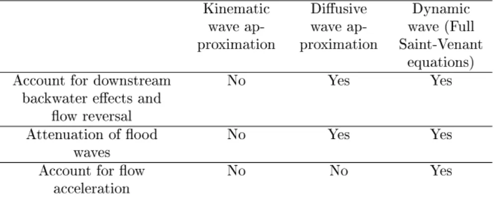
Table 2.1 gives an overview of some characteristics of the various approximations of the Saint-Venant equations.

Kinematic wave ap-proximation Diusive wave ap-proximation Dynamic wave (Full Saint-Venant equations) Account for downstream

backwater eects and ow reversal

No Yes Yes

Attenuation of ood

waves No Yes Yes

Account for ow

acceleration No No Yes

Table 2.1: Overview of some characteristics of various approximations of the Saint-Venant equations (Adeyemo, 2007).

The data required for the solution of the shallow water wave equations includes cross-sectional information, roughness coecients, boundary conditions and any internal structures. For some catchments, this information may not be available. Generally, approximations to the shallow water wave equations will require less demanding data requirements (Zoppou, 2001).

2.4.2.1 Urban drainage models

Traditional sewer systems are networks of conduits and manholes. Surcharge occurs in the presence of a closed conduit, which instead of acting as an open channel, as would normally happen, becomes full and acts as a conduit under pressure (Zoppou, 2001) (Figure 2.4). In these cases, the water will rise above the ground level if pressure is sucient, creating an overow where the excess volume of ow becomes surface runo. Water from the pipe system may ow to the streets through a manhole when ooding takes place and, conversely, surface ooding water in the street system can ow through the manholes to the pipe system when water in the pipe system is drained.

2.4. Modelling approaches in urban drainage

Figure 2.4: Stages of sewer surcharge (Schmitt et al., 2004)

Most of the traditional urban drainage models store ood water from the under-ground system in a virtual reservoir when surcharge water from a pipe system ows into the street system, and the stored volume returns to the pipe once the system resumes free surface ow (Figure 2.5).

(a) (b) (c)

Figure 2.5: Traditional approaches when water reaches the surface a) water is lost b)water is stored and returns later to the system c) virtual reservoir (Wallingford Software 2009)

An important development was achieved by Djordjevic et al. (1991) who cre-ated a method to simultaneously solve storm sewer and street ows equations. They used the diusive wave approximation of the full Saint-Venant equations to model both ow phases. Their work highlights the fact that the ows in the storm sewers can be signicantly aected if excess volumes are allowed to ow along the street, instead of being stored in ctitious basins, above the surchar-ging manhole.

Maksimovic and Prodanovic (2001)concluded for the need of a new methodo-logy for simulating the storage of surface ooding on the street system, instead of using a virtual reservoir approach at each computational nodal point on the surface. Through the application of GIS features such as a DEM and a simula-tion module, modelling of the real storage and routing of surface ooding would be accomplished.

Dual drainage concept

The need to correctly predict the extent of a ood led to the development of the dual drainage concept. The concept was introduced in the eighties in North America and consists in an urban drainage through both a minor system (drainage sewer network, including the manholes and the inlet connections) and a major system (above ground ood pathways, natural and man-made, including both open and culverted watercourses) (Figure 2.6). The integrated use of these two sub-systems is referred to as dual drainage Djordjevic et al. (2005). The major system is often modelled by either one-dimensional (1D) or two-dimensional (2D) models. The way in which the surface network is discretised as a 1D model is by considering the domain as a set of nodes connected by links (Nasello and Tucciarelli, 2005). The nodes represent the channel junctions, ponds or crossings, connected by links, mainly the open channels. In 2D models the domain is discretised as a coordinate system of nodes (i.e. grid of points or mesh), where each point on the grid is represented by spatial coordinates (X, Y, Z). Regarding the man-made pathways of an urban mesh, 1D models constitute a good approximation provided the ow on the surface remains within the street prole (Mark et al., 2004). However, if the ow overtops the curb levels, 2D models are the preferred choice. While the minor system is designed to carry the runo from a storm of 210 year return frequency, the surface system is designed to deal with events of 25100 year return frequency (Schmitt et al., 2004).

2.4. Modelling approaches in urban drainage

Figure 2.6: Idealised surface and storm sewer ow components in dual drainage systems (Djordjevic et al., 1999).

The minor system in urban ooding has been modelled exclusively by 1D models given the preferential direction of the ow along the longitudinal pipe axis. If the water level remains lower than the pipe crown, then the water ow inside the pipe remains free-surface. However, if the water level reaches the pipe crown, the water ow will become pressurised, and then it is possible to have both types of ows occurring at the same time. To account for this type of ow shift, the Preissmann slot concept (Preissmann, 1961) is adopted in most models (Butler and Davies, 2011)(e.g. MOUSE, XPSWMM, PCSWMM and InfoWorks). The Preissmann slot concept permits the modelling of free-surface ows and allows the Saint-Venant equations (valid for free surface ow) to be applied to pressurized ow (Figure 2.7) .

Figure 2.7: Preissmann slot (Preissmann, 1961)

An integrated model is said to exist whenever a model links a major to a minor system by elements which allow the ow transfer between both systems in a synchronised manner. This type of models can be further classied into partially and fully integrated. In fully integrated models, the same time step is used to couple the two systems and a time step limiter is generally applied in order to ensure stability (e.g. Courant condition). In contrast, in the partially integrated approach both models run separately and the ow exchange is only done at specic time steps (synchronisation) (Schmitt et al., 2004; Chen et al., 2007). Conservation of energy and continuity are used by most models. Matching both water levels in both systems subtracted from any local losses and kinetic energy allows for energy conservation. The conservation of momentum is seldom applied due to the diculty in transferring momentum from a vertical direction to a horizontal and vice-versa.

Figure 2.8 shows the interactions in various stages in modelling approaches for a ooded urban drainage system.

2.4. Modelling approaches in urban drainage

Figure 2.8: Interactions between various stages in the modelling approach for a ooded urban drainage system (Mark et al., 2004).

According to Allitt et al. (2009) one of the main problems of 1D1D models (i.e. 1D model of the sewer network coupled with a 1D model of the surface) is visualisation: diculty of presenting the results in a manner in which they are easily understood. One potential solution for this are the ood compartments of Infoworks. 1D1D models should only be trusted when the nature of surface ow is essentially one-dimensional, i.e. where there is little uncertainly about drainage routes and where the ow outside larger ponds is mostly limited to the road width. This situation is sometimes referred to as conveyance ooding and is more likely to occur in areas with steeper topography and would result in relatively high ow velocities.

Two dimensional models involve a lower degree of averaging of fundamental hydraulic equations than 1D models, therefore the former can be considered as a more realistic description of ow conditions. This is particularly the case when surface ows are not limited to well-dened routes along roads or surface channels and when ooding is mainly a ponding process with relatively slow water movement. 1D2D modelling is also the best choice when it comes to extreme events when most of the urban surface is covered with excessive ood depths. 1D1D models are less time consuming than 1D2D models which make the more reliable for ood forecasting.

to combine dierent approaches such that dierent parts of the catchment are simulated by combining elements of 1D, 1D-1D and 1D-2D techniques within a single model (Figure 2.9).

Figure 2.9: Conceptualisation of Integrated Urban Drainage Model Blanksby et al. (2007)

According to Blanksby et al. (2007) there are four basic types of urban drainage model: i) Simple models; ii)1D drainage system models of pipes and channels; iii) Integrated 1D surface and drainage system models; and iv) linked 2D sur-face and 1D drainage system models. In the Pitt Report (2008), the following models were used: i) Topographic index analysis: a basic terrain model with no rainfall input. As there is no correlation between the model's outputs and areas of known ooding, it has few practical applications. ii) 2D overland routing of a uniform rainfall event: the model does not allow for dierences in rainfall, and presumes there are uniform capacity to drain water independently of the area being considered. It could be used for high level analysis but substantially over-estimates the extent of ooding. iii) Decoupled sewer model and 1D overland routing: the model takes account of the eect of drainage by using a detailed sewerage network model. It is the most precise method of identifying properties on water company registers but underestimates the spatial extent of ooding; iv) Decoupled sewer model and 2D overland routing: the model includes 2D

2.4. Modelling approaches in urban drainage surface runo data and detailed sewerage network data, but excludes the as-sessment of below-ground ooding mechanisms. It produces a more precise estimate of the spatial extent of ooding but fails to identify some properties on water company registers; v) Coupled sewer model and 2D overland routing: the model combines surface runo data, detailed sewerage network data and a full 2D model of above-ground ooding.

2.4.2.2 Existing Flood Models

In the previous section the shallow water equations, also known as Saint Venant equations, were presented. They are based on the mathematical conservation laws for mass and momentum, both in 1D and 2D; they are considered the most reliable models for free surface ow. Examples of commercial packages that use these equations for surface water modelling are Infoworks, Mike Flood, Tuow and Sobek.

Several authors have presented research works carried out with these packages and other softwares. For example Vaes et al. (2004), Gutierrez-Andres et al. (2008) and Leitao (2009) used the 1D1D model INFOWORKS CS for overland ow paths modelling and ood mapping whilst Leandro (2008) used 1D1D ver-sion of SIPSON ((Djordjevic et al., 1999)). Two dimenver-sional models to simulate surface runo have been integrated into urban drainage models by several au-thors, including MOUSE-MIKE 21 which integrates sewer model MOUSE with the 2D MIKE 21 (Carr and Smith, 2006), Sobek Urban which combines 1D model SOBEK Flow and 2D Delft FLS (Bolle et al., 2006), TUFLOW (Phillips et al., 2005) and SIPSON-UIM (Chen et al., 2007).

In these works several recommendations have been made for modellers: pipe slopes were recognised as a potential cause of numerical problems, and the need to limit small water depths because there was a loss of accuracy in the surface network for high velocities (Vaes et al., 2004); Lhomme et al. (2006) point out that the distribution of ows at crossroads and the disregarding of backwater eects were major source of errors in the 1D models of the surface; Chen et al. (2007), Leandro (2008) and Bolle et al. (2006) showed the need to correctly model the ow between the surface and the sewer system.

The use of these models has been increasing (Krupka et al., 2007) but their application to real-world problems is limited by computer requirements. In fact, one of the main problems of the models based on the shallow water equations is the time required to run hydraulic simulations (Pender and Liu, 2011). When inundation over very large areas requires to be simulated, these models can take very long time.

Although there are several new developments in hardware and software (e.g. parallel computing) that can help to improve simulation time, there are new types of alternative models, called rapid ood models based on storage cells (Figure 2.10). Storage cell code models the oodplain as a series of discrete basins, using simple relations such as the Manning equation, to calculate the ow between cells. These models are not physically based, but keep many of the advantages of full two-dimensional schemes, with a reduction in terms of computational cost. However these models have some disadvantages: the propagation speed of the inundation front over the oodplain has been shown to be highly dependent on the model grid scale and insensitive to oodplain friction (Hunter et al., 2006); ood water velocity cannot be predicted and; the same volume of water with dierent inow hydrographs will produce the same nal ood extent (Pender and Liu, 2011).

Figure 2.10: Storage cell procedure scheme (Bates, 2012)

Some examples of this type of model are LISFLOOD-FP (Horritt and Bates, 2002), Cellular Automata (CA) (Guo et al., 2007), Rapid Flood Spreading Model (RFSM) (Lhomme et al., 2009), Flowroute (Butler et al., 2009). Re-cently Pender and Liu (2011) presented a new RFSM that accounts for the rate of ood inow, and the prediction of maximum velocity within each oodplain cell.

Lhomme et al. (2009) compared RFSM with Tuow: while Tuow needs some hours to run some events, the RFSM only needed a few seconds, with a minimum depth deviation. Similar results were obtained by Fewtrell et al. (2009) and Asselman et al. (2009).

2.4.3 Automatic Overland Flow Delineation (AOFD)

Maksimovic et al. (2009) presented a recent progress in modelling of overland ow in urban environment caused by pluvial ooding. The concept adopted in

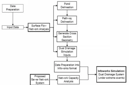
2.4. Modelling approaches in urban drainage the work was based on the GIS centred analysis of a conditioned DTM and DEM, crucial for identication of ood vulnerable areas (mainly ponds), so that the features of the catchment can be derived and the geometric characteristics of the preferential paths determined. The AOFD (Automatic Overland Flow Delineation) tool uses a new methodology to generate a model of the overland ow. The tool automatically creates the overland ow network to enable its interaction with the sewer drainage system.

The tool consists of several GIS routines that analyse and quantify the surface overland ow network of urban catchments based on input data e.g. master map, elevations, sewer network. The outputs were designed to give an additional surface pathways' network in order to improve the accuracy of the simulation model of urban ooding. The analysis can be divided in four main steps: (i) ponds' delineation; (ii) pathways delineation; (iii) pathways geometry; and (iv) generation of input les for urban drainage models.

The methodology developed searches the entire DTM and seeks and identies the local low points. Based on the DTM, the pond boundary for each low point is delineated and the natural exit point is identied as the termination critera. The exit point acts as the starting point for the ood pathway over the catchment surface.

Starting at the natural exit points of the identied ponds or surcharged man-holes, the analysis determines pathways by preferential ow directions based on terrain slope, taking into account the presence of buildings and other features that are included in the DEM (Figure 2.11).

Pond 2 Pond 3 Pond 1 (iv) Pond 4 (iii) (i) Manholes Manholes (ii) (vii) (v) (vi)

Figure 2.11: Types of surface pathways calculated from the DEM (Maksimovic et al, 2009)

According to Maksimovic et al.(2009), the types of surface pathways generated by the AOFD tool are: