Entry Deterrence in Durable-Goods Monopoly
∗
Heidrun C. Hoppe
University of Hamburg
In Ho Lee
University of Southampton
January 14, 2000
AbstractSome industries support Schumpeter’s notion of creative destruction through innovative entrants. Others exhibit a single, persistent technological leadership. This paper explores a durable-goods monopolist threatened by entry via a new generation of the durable good. It is shown that the durability of the good either acts as an entry barrier itself or creates an opportunity for the incumbent firm to deter entry by limit pricing. As a consequence, the industry tends to remain monopolized, with successive generations of the durable good being introduced by the incumbent monopolist. We show that entry deterrence by limit pricing can lead to underinvestment in innovation.
Keywords: Entry deterrence, durable goods monopoly, Coasian dynamics, innovation. JEL classification: D420, L110
∗We would like to thank David Audretsch, Robin Mason, Roy Shin, Juuso V¨alim¨aki and seminar participants
1
Introduction
This paper explores a durable-goods monopolist threatened by entry via a new generation of the durable good. It will be shown that the durability of the good either acts as an entry barrier itself or creates an opportunity for the incumbent firm to deter entry by limit pricing. As a con-sequence, the industry tends to remain monopolized, with successive generations of the durable good being introduced by the incumbent monopolist. These results may have implications for empirical studies on innovation and entry dynamics as well as antitrust policies.
It is often argued that Coasian pricing dynamics in a durable-goods monopoly warrants the competitiveness of that industry, even in the absence of competitors. The reason is that a durable-goods monopolist will optimally reduce the price once high-valuation consumers have bought. Knowing this, even high-valuation consumers will postpone their purchases. Accord-ingly, prices converge to the competitive level as price adjustments become more frequent. But the monopolist may attempt to avoid the time-inconsistency problem by limiting the effective durability of the good. Different possibilities are discussed in the literature: (i) contracts, i.e. renting the product rather than selling it (Coase (1972), Bulow (1982)), (ii) physical obso-lescence, i.e. producing shorter useful product lives (Coase (1972), Bulow, (1986)), and (iii) innovation, i.e. inventing and introducing a new generation of the good (Waldman (1993), Fudenberg and Tirole (1998), Lee and Lee (1998)).
However, the picture may change when the existence of a potential entrant is taken into account. As Bucovetsky and Chilton (1986) and Bulow (1986) demonstrate, the incentives to rent or produce short-lived products may be reversed when the monopolist is faced with a future entrant who can produce the same good. Higher durability limits future demand and, hence, future profits. This may prevent entry when entry is costly.
The present paper focuses on the interplay between Coasian pricing dynamics and the in-centives for innovation in a durable-goods monopoly when potential competitors threaten to innovate as well. More precisely, we ask whether the durability of the goods creates any op-portunities for a monopolist to prevent innovative firms from entering the industry, and whether innovation investments in durable-goods monopolies under entry threat are socially efficient.
The importance of these questions is exemplified by the worldwide interest in the current antitrust case of the United States versus Microsoft Corporation1. Microsoft is accused of un-lawfully maintaining its monopoly power by anticompetitive behavior in the software market.
In this respect, Liebowitz noted in the Wall Street Journal Europe2 that “the government be-lieves that Microsoft has merely leveraged its control over operating systems to dominate the software market even where its products are clearly inferior to the alternatives.” “Instead,” he argues, has “Microsoft achieved its success the old-fashioned way - with better products (...) that have nothing to do with antitrust violations.”
We construct a two-period model in which a new generation of a durable good can be in-vented and introduced in the second period by the incumbent monopolist or a potential entrant. The old generation of the durable good lasts two periods so that consumers who buy it in the first period can use it until the second period. The new generation of the durable good is char-acterized by a higher quality. Consumers can consume only one unit of the durable good in each period and have uniformly distributed quality tastes. They can prove the purchase of the old generation to be eligible for an upgrade discount on the new one.
First, we demonstrate that preemptive innovation cannot prevent entrants from taking over the technological leadership in the absence of effective patent protection. Our finding is anal-ogous to Judd’s (1985) result on spatial preemption. The intuition that underlies both of them is that a multiproduct incumbent firm may optimally respond to entry into one market segment by withdrawing his product in that segment if postentry price competition reduces demand in another, monopolized segment of the market. In the context of quality improvement, the argu-ment obviously holds for durable-goods industries as well as non-durable-goods industries, as long as the demand for the incumbent’s original product is positively related to the price for the high-quality version of the good.
Second, we show that a durable-goods monopolist may credibly deter entry by means of limit pricing. Lowering the price of the old generation of the durable good in the first period increases first-period demand and hence the number of second-period consumers who are will-ing to pay only for the incremental utility derived from the new generation of the product over the old one. Interestingly, this may prevent the entrant from investing in innovation without necessarily making the innovation investment unattractive to the incumbent. The reason is that innovation by the potential entrant results in price competition with vertically differentiated products, while innovation by the incumbent yields a multiproduct monopoly. In particular, we show that the entrant would never implement a cross-upgrade policy due to competitive pressure, whereas the multiproduct monopolist may find it optimal to offer upgrade discounts
in order to price discriminate between former and new customers. Since competition dissi-pates post-innovation profits, the entrant’s incentive for innovation is smaller than that of the incumbent monopolist.
Third, we demonstrate that entry deterrence by limit pricing may lead to consumer leapfrog-ging. That is, consumers who have bought the old product do not upgrade to the new version, while others who have not obtained the old version decide to purchase the new one.
Finally, we show that innovation investments in a durable-goods monopoly under entry threat are not necessarily desirable from a welfare point of view. When innovation occurs, inefficiency can take either of two forms: the incumbent may be the single innovator even though the entrant has lower innovation costs, and vice versa. Furthermore, we show that any entry-deterrence equilibrium without innovation implies underinvestment in innovation.
The findings appear largely consistent with empirical observations in the software industry mentioned above. There is a common consent that Microsoft holds a virtual monopoly. But, as Schmalensee notes in the Boston Globe, “a real monopolist - one who extracted the last dollar of profit from consumers - would charge hundreds of dollars more for the software that runs modern PCs.”3 We argue that Microsoft charges low prices to make entry via a new generation unattractive by flooding the market with the old one. Such a view is supported by Microsoft’s mission “a PC on every desk and in every home, running Microsoft software”, and the observation that it is often Microsoft that brings the new generation of products to the market, and not a competitor. Moreover, upgrade discounts are typically offered by Microsoft on its own new products, whereas cross-upgrade pricing is rarely observed.
Ever since Schumpeter (1942), there has been a continued interest in the factors that influ-ence entry into monopolized industries through innovation, as is expressed, for instance, by the prominent debate between Gilbert and Newbery (1982) and Reinganum (1983). This literature, however, focuses on non-durable-goods industries. The results indicate that the monopolist will deter entry by preemptive patenting when he is more concerned with the dissipation of post-entry profits (known as the efficiency effect) than the cannibalization of his current monopoly rents (known as Arrow’s (1962) replacement effect), where the latter effect may matter when there is uncertainty about the innovation date. In our model, the innovation technology is de-terministic, which eliminates the replacement effect. While patent protection and, hence, the possibility of preemptive patenting is ignored as well, we show that a durable-goods monopolist
has nevertheless the means to prevent entry by credible preemptive action when the efficiency effect matters. The monopolist may charge a low price to flood the market with the old genera-tion of the good before entry takes place.
The idea behind limit pricing in our model differs from that put forth by Milgrom and Roberts (1982). In Milgrom and Roberts’ model, limit pricing is based on asymmetric informa-tion between the entrant and the incumbent about the incumbent’s cost of producinforma-tion, while our paper assumes complete information. Furthermore, in our paper limit pricing, when exercised, removes the possibility of entry unambiguously. This is consistent with the original idea of limit pricing due to Bain (1949). By contrast, Milgrom and Roberts’ result is ambiguous on the probability of entry.
Complete-information limit pricing as an entry-deterrence practice has previously been at-tributed to suppliers of network goods. Katz and Shapiro (1992) and more recently Fudenberg and Tirole (1999) show that an incumbent may charge low prices to build a large installed base of users of a network good in order to deter entry with an incompatible product. These pa-pers, however, assume away any Coasian pricing dynamics and incentives for upgrade pricing which are associated with many durable-goods industries. Entry deterrence by limit pricing relies therefore solely on the presence of network externalities in the demand for compatible products. By contrast, our paper attributes entry deterrence by limit pricing solely to the dura-bility of the goods in the complete absence of any network externalities. We believe that the arguments are complementary in nature.
The paper is organized as follows. In the next section we present a two-period model of a durable-goods monopoly threatened by entry through innovation. Section 3 analyzes the subgames after the innovation decisions. Section 4 provides main analysis of the whole game. Section 5 discusses welfare implications, and Section 6 concludes.
2
The Model
Consider a two-period model of a durable-good market. In period 1, the market is monopolized by an incumbent,I. The incumbent produces a durable good, associated with quality levelsL, that lasts two periods after which it vanishes. Between period 1 and period 2, the incumbent can invest in innovation, which enables him to produce a new generation of the good, characterized by the higher quality level sH = (sL+s∆), s∆ > 0. Hence, conditional on innovation, the
incumbent may sell both generations of the good in period 2, the low-quality one and the high-quality one. There is also a potential entrant,E. By investing in innovation, the entrant is able to produce and sell the new generation of the good with qualitysH in period 2. Variable costs of production are independent of quality and set equal to zero. Following Fudenberg and Tirole (1998), we assume that the quality improvement is not too large:4
sL > s∆ (A1)
It is further assumed that the firms cannot change the quality when the good is already produced. On the demand side, there is a continuum of consumers with different utility from con-sumption of the durable good. Each consumer is associated with a typeθwhich is known only to himself. Consumer types are uniformly distributed over the range [0,1]. Consumers may consume at most one unit of the durable good in each period. The consumer of type θ gets utilitysiθ from consumption of the good of qualitysi per period,i = L, H.There is no exter-nality among the consumers such as, for example, a network effect. Consumers and firms have a common discount factor which is normalized to1. There is no second-hand market.
The firms and consumers face the following multi-stage game. At the beginning of pe-riod 1, the incumbent sets a price for the original durable good. Consumers choose whether to purchase the good in period 1 or not. Hence, after period 1, the market divides into the following two segments: (i) the “upgrade market”, which consists of the consumers who have purchased the good in period 1 and may want to upgrade in period 2 if that is an option, and (ii) the “new-purchase market”, which consists of the consumers who have not purchased in period 1. Between the end of period 1 and the beginning of period 2, the incumbent and the potential entrant simultaneously choose whether to invest in innovation which encompasses the invention and introduction of a new generation of the product to the market. The innovation costs are KI ≥ 0andKE ≥ 0 for the incumbent and the entrant, respectively. We allow the firms to observe the outcome of innovation game instantaneously. At the beginning of period 2, each firm decides whether to withdraw any product that it is able to produce from any market at zero cost5, and sets a price for each product it wishes to offer in any market. In particular, each
4The assumption is necessary for the uniqueness of equilibrium.
5We follow Judd (1985) in allowing for an intermediate exit stage. Exit is assumed to be costless to apply Judd’s
argument on the non-credibility of spatial preemption and thereby obtain a unique solution for the second-period pricing subgame. Without this assumption, a certain parameter range would admit multiple equilibria, where one of them could be part of an entry-deterrence equilibrium similar to that in Gilbert and Newbery’s (1983) model
potential supplier of the new generation of the good can choose to price discriminate between consumers with respect to purchase history. That is, we allow the incumbent to give an upgrade discount to the consumers in the upgrade market, and the entrant to give a cross-upgrade dis-count to former customers of the incumbent. However, the pricing decision is subject to the incentive compatibility constraint that the upgrade price cannot exceed the new purchase price, since consumers in the upgrade market can pretend not to have purchased previously. If the incumbent wishes to offer the original durable good in period 2, he may set a new price for it. Finally, consumers choose in period 2 whether to buy any product that is offered.
We use the subgame-perfect equilibrium as the solution for the game.
3
Sales in Period 2
As is standard in the analysis of subgame-perfect equilibrium, we start with the examination of the second-period play. It comprises two sales decisions by each firm, i.e the decision in which market to offer any product that can be produced plus the decision of how to price the respective product, and the purchase decisions of the consumers. These decisions depend on the sales history in period 1. For this, it is easy to verify the following monotonicity property. If the consumer of typeθ1prefers to purchase in period 1, then all consumers with typeθ ≥θ1prefer to purchase in period 1 (Fudenberg and Tirole (1998 [Lemma 4])). Hence, we can represent the sales history by the type of the cutoff consumer θ1. Furthermore, the second-period subgame is associated with four possible innovation histories, which are denoted as follows: N denotes the history in which no firm has innovated; I and E denote the histories in which only the incumbent or only the entrant has innovated, respectively; andB denotes the history in which both firms have innovated. We define four subgamesΓN,ΓI,ΓE,ΓBfor each innovation history, respectively. In this section, we will solve each of them separately.
3.1
Γ
N: No Innovation
When no firm has innovated, the incumbent may choose to sell to consumers who have not purchased in the past, i.e. consumers of typesθ < θ1. Let pL denote the second-period price for the original, low-quality good. The incentive constraint for the marginal consumer is given
of preemptive patenting. But even in that case, the equilibrium that is unique under costless exit would remain an equilibrium.
byθ2sL−pL= 0.Taking account of the incentive constraint, the incumbent’s problem is max pL pL(θ1− pL sL ) (1)
subject topL/sL< θ1, which is solved by
pL =
1
2sLθ1. (2)
3.2
Γ
I: Innovation by the Incumbent
This subgame has been analyzed by Lee and Lee (1998) for the case of two types of consumers and by Fudenberg and Tirole (1998) for a general distribution of consumer types. Our analysis for a uniform distribution of consumer types largely confirms their results. In addition, we obtain an explicit characterization of the equilibrium which is crucial for the analysis of the entire game.
Let pU andpH denote the price of the new, high-quality product offered to consumers in the upgrade market and the new-purchase market, respectively. For a given first-period cutoff consumer,θ1, the incumbent can pursue the following sales strategies. First, the incumbent may choose to price discriminate between consumers in the upgrade market and consumers in the new-purchase market. Since upgrade consumers can pretend not to have purchased in period 1, the incumbent must take the incentive compatibility constraintpU ≤pH into account. Second, he can offer the new product to consumers in both markets at a uniform pricepU =pH. Third, he can choose to withdraw the new product from the new-purchase market and sell it only to consumers in the upgrade market. In addition, he may choose to sell the old product at price
pL. However, since production of either quality is costless, it can easily be shown that the incumbent finds it optimal to sell only the new product, as long as no incentive compatibility constraint is binding. The next proposition indicates how the optimal strategy of the incumbent encompasses the alternative sales strategies depending on the parameterθ1.
Proposition 1 Consider subgameΓI. Define
z1 ≡ s∆(sL+s∆−√s∆ p (sL+ 2s∆)) s∆sL+s2L−s2∆ z2 ≡ s∆ sL+s∆
where0< z1 < z2 <1/2.
1. Ifz2 < θ1 ≤1, the incumbent sells the new product in the upgrade market at the price
pU = ( θ1s∆ if 12 < θ1 ≤1 1 2s∆ ifz2 < θ1 ≤ 1 2 (3)
and in the new-purchase market at the price
pH =
1
2(sL+s∆)θ1, (4)
wherepU < pH for z2 < θ1 <1.
2. Ifz1 < θ1 ≤z2, the incumbent sells the new product in both markets, the upgrade market
and the new-purchase market, at the uniform price
pU =pH = 1 2s∆ sL+s∆ sL+ 2s∆ (1 +θ1). (5)
3. If 0 ≤ θ1 ≤ z1, the incumbent sells the new product only in the upgrade market at the
price6
pU =
1
2s∆ (6)
and the old product in the new-purchase market at the price given by (2).
Proposition 1 reveals that the incumbent will price discriminate between customers with different purchase history by offering an upgrade discount to those who have purchased in period 1, provided that the upgrade market is not too large (statement 1). Two effects matter for this result: First, consumers in the new-purchase market are willing to pay (sL+s∆)θ, while those in the upgrade market are willing to pay onlys∆θfor the incremental utility. This implies a higher new-purchase price (the reservation-utility effect). Second, as the upgrade market gets large, the maximal valuation among the consumers in the new-purchase market decreases. This drives the new-purchase price down relative to the upgrade price (the ratchet effect). For a large upgrade market, the ratchet effect dominates the reservation utility effect such that the
6Forθ
1 =z1, the incumbent is indifferent between the policies described in statements 2 and 3. We assume
incentive compatibility constraintpU = pH is binding. The incumbent charges then a uniform price for the new product (statements 2 and 3). When the upgrade market gets very large, the optimal uniform price will exceed the maximal willingness to pay of any consumer in the new-purchase market. The incumbent can therefore gain from foregoing sales of the new product in the new-purchase market entirely (statement 3).
Finally, we shall analyze whether there are consumers who possess the old product and do not upgrade to the new version, while there are others who have not bought the old version and decide to purchase the new one. Such consumer leapfrogging implies that a consumer with a higher valuation may use a product of lower quality than a consumer with a lower valuation. The analysis might therefore be of an independent interest in the context of technology adoption as discussed in the growth literature.
Corollary 1 Leapfrogging occurs inΓI ifz
1 < θ1 <1/2.
Corollary 1 indicates that leapfrogging may take place in ΓI for a range of the first-period sales history. Note that this does not imply that leapfrogging occurs in the overall game.
3.3
Γ
E: Innovation by the Entrant
When the entrant is the only innovator, he can monopolize the upgrade market but faces price competition between vertically differentiated goods in the new-purchase market. While the incumbent’s strategy set is simply a choice ofpL ≥0, the entrant’s strategy set is composed of the following sales policies. First, the entrant can price discriminate between the consumers in the new-purchase market and those in the upgrade market by giving a cross-upgrade discount
pU < pH. Second, he can charge a uniform price in both markets pU = pH. Third, he can
forego sales in the new-purchase market completely. As a preliminary step, we show in the next lemma that a cross-upgrade discount is never optimal for the entrant. Proposition 2 then summarizes the equilibrium behavior inΓE.
Lemma 1 Price discrimination between consumers with respect to purchase history is never
optimal for the entrant.
Lemma 1 is due to the competition between the entrant and the incumbent in the new-purchase market which calls for a low new-new-purchase pricepH. The proof of the lemma estab-lishes that this competition effect together with the ratchet effect always dominate the reserva-tion utility effect so that the incentive compatibility constraintpU ≤pH is always binding.
Proposition 2 Consider subgameΓE. Define x1 ≡ (7√2−8)sL+ (8 √ 2−8)s∆ 8sL+ 8s∆ x2 ≡ 2sL+ 2s∆ 5sL+ 6s∆ x3 ≡ 2sL+ 2s∆ 3sL+ 4s∆ where0< x1 < x2 <1/2< x3 <1.
1. Ifx3 < θ1 ≤1, the entrant sells the new product in both markets at the uniform price
pH =pU = 2s∆
sL+s∆
3sL+ 4s∆
(7)
such that the first-period cutoff type θ1 prefers to buy the new product. The incumbent
sells the old product at the price
pL=s∆
sL
3sL+ 4s∆
. (8)
2. Ifx2 < θ1 ≤x3,the entrant sells the new product in both markets at the uniform price
pH =pU =s∆θ1 (9)
such that the first-period cutoff typeθ1 is indifferent between buying the new product or
not. The incumbent sells the old product at the price7
pL= 1 2s∆ sL sL+s∆ θ1. (10)
3. Ifx1 < θ1 ≤x2, the entrant sells the new product in both markets at the uniform price
pH =pU = 2s∆
sL+s∆
7sL+ 8s∆
(1 +θ1) (11)
such that the first-period cutoff typeθ1prefers not to buy the new product. The incumbent
7Forθ
1=x3, the entrant is indifferent between the policies described in statements 1 and 2 of this Proposition.
We assume that forθ1 =x3 firms coordinate on the strategies specified in statement 2, since it yields a higher
sells the old product at the price
pL =s∆
sL
7sL+ 8s∆
(1 +θ1). (12)
4. If0≤θ1 ≤x1,the entrant sells the new product only to consumers in the upgrade market
at the price
pU =
1
2s∆. (13)
The incumbent sells the old product at the price given by (2).8 5. The entrant’s profit inΓE is continuous and weakly increasing inθ1.
The proposition exhibits an interesting discontinuity at θ1 = x1. As θ1 falls from above
x1 below that value, the entrant stops selling the new product to new-purchase consumers, and the price of the new durable good jumps upwards to pU = (1/2)s∆ (statements 3 and 4). The reason is that for a sufficiently large upgrade market, i.e. θ1 ≤ x1, it is profitable for the entrant to avoid competition in the new-purchase market. Note that the optimal upgrade price does not depend on the low end of the upgrade market, when the upgrade market is already of substantial size (statement 4). For a smaller upgrade market, i.e. θ1 > x1, the entrant is subject to substantial competitive pressure from the incumbent who continues selling the old durable good. The competitive pressure prevents the entrant from price-discriminating between upgrade consumers and new-purchase consumers (statements 1-3 and Lemma 1).
Finally, similar to the previous subsection we analyze the consumers’ equilibrium purchase decision and check whether leapfrogging is possible in subgameΓE.
Corollary 2 Ifx1 < θ1 < x2, leapfrogging occurs inΓE.
The corollary shows that consumer leapfrogging may occur in ΓE for a range of the first-period sales history. The range is similar to the case ofΓI, but it is narrower.
8Forθ
1 = x1, the entrant is indifferent between the policies described in statements 3 and 4. We assume
that forθ1 =x1firms coordinate on the strategies specified in statement 4, since it yields a higher profit for the
3.4
Γ
B: Innovation by Both Firms
Consider the subgame where both firms have innovated. In this case, the incumbent can sell both goods, the old one and the new one, while the entrant can sell only the new version. We will demonstrate, however, that the incumbent prefers to offer only the old product.
Proposition 3 In subgame ΓB, it is optimal for the incumbent to withdraw the new product
entirely and sell only the old product.
Proposition 3 describes a striking result. When both firms introduce the new version of the durable good, the optimal response of the incumbent is to withdraw the new product from both markets, the upgrade market and the new-purchase market. The result can be explained as follows. If the incumbent remains in both markets, Bertrand price competition drives the new-purchase price and the upgrade price down to zero. As a consequence, the price for the old product is zero as well. Hence, each firm makes zero profits. It is obvious that the entrant cannot gain by exiting either market, which yields zero profits as well. However, the incumbent may want to avoid the price competition in the new-purchase market in order to generate positive profits with the old product. Since the old product is directly competing against the new one, the incumbent has an incentive to withdraw the new product from the new-purchase market.9
Moreover, the incumbent can do even better by withdrawing the new product from the upgrade-market as well and offering only the old product, as with history E. To understand this point, remember that for historyEthe entrant charges a uniform price for the new product in both markets as the incentive compatibility constraintpU ≤pH is binding (Lemma 1). This price is higher than the entrant’s optimal (unconstrained) new-purchase price. It is clear that the incumbent benefits from a higher price charged by its rival. Hence, when both markets are linked by the incentive compatibility constraint, as with historyE, the incumbent is actu-ally better off relative to when markets are separated, as with history B and free upgrading. Corollary 3 follows immediately from Proposition 3.
Corollary 3 InΓBthe incumbent and the entrant make the same profit as inΓE. Leapfrogging
occurs under the same circumstances as inΓE.
It is interesting to note that this result implies that innovation has no preemptive power in deterring an entry, in contrast to the previous debate between Gilbert and Newbery (1982) and
9A similar result has been obtained by Judd (1985) for a multiproduct incumbent with horizontally
Reinganum (1983). The difference follows from the multiple product feature of the present model.
4
Sales in Period 1
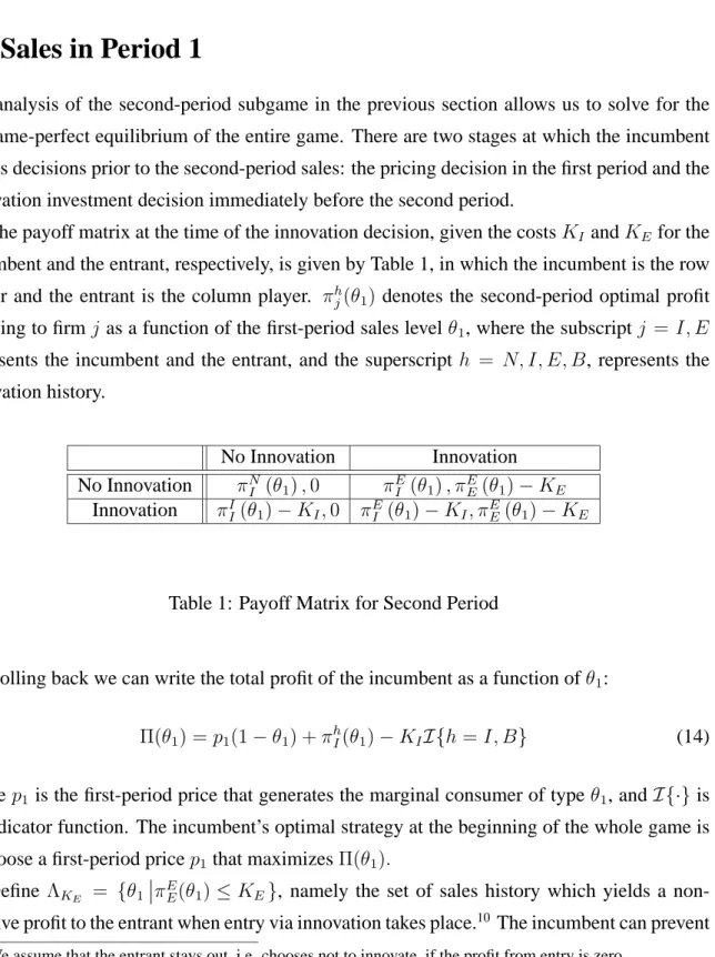
The analysis of the second-period subgame in the previous section allows us to solve for the subgame-perfect equilibrium of the entire game. There are two stages at which the incumbent makes decisions prior to the second-period sales: the pricing decision in the first period and the innovation investment decision immediately before the second period.
The payoff matrix at the time of the innovation decision, given the costsKIandKE for the incumbent and the entrant, respectively, is given by Table 1, in which the incumbent is the row player and the entrant is the column player. πhj(θ1)denotes the second-period optimal profit accruing to firmj as a function of the first-period sales level θ1, where the subscript j = I, E represents the incumbent and the entrant, and the superscript h = N, I, E, B, represents the innovation history.
No Innovation Innovation
No Innovation πN
I (θ1),0 πEI (θ1), πEE(θ1)−KE Innovation πII(θ1)−KI,0 πEI (θ1)−KI, πEE(θ1)−KE
Table 1: Payoff Matrix for Second Period
Rolling back we can write the total profit of the incumbent as a function ofθ1:
Π(θ1) = p1(1−θ1) +πIh(θ1)−KII{h=I, B} (14) wherep1 is the first-period price that generates the marginal consumer of typeθ1, andI{·}is an indicator function. The incumbent’s optimal strategy at the beginning of the whole game is to choose a first-period pricep1that maximizesΠ(θ1).
Define ΛKE = {θ1
πEE(θ1)≤KE}, namely the set of sales history which yields a non-positive profit to the entrant when entry via innovation takes place.10 The incumbent can prevent
entry by setting the first-period price in such a way that all consumers of typeθ ≥ θ1 ∈ ΛKE purchase in the first period. We callΛKE the no-entry set.
Using Bain’s terminology, we distinguish between three forms of first-period behavior:
blockaded entry, where the incumbent chooses a first-period price as if there were no entry
threat, but no entry occurs; deterred entry, where entry cannot be blockaded, but is prevented through limit pricing; and accommodated entry, where the incumbent prefers a first-period price that does not prevent entry, and entry occurs. The subgame-perfect equilibrium of the en-tire game has different properties, depending on whether entry takes place or not. We analyze first the no-entry equilibrium in which entry is either blockaded or deterred, then the entry equi-librium in which entry is accommodated, and finally, we examine how the incumbent chooses in the first stage between the two equilibrium paths if both are available.
4.1
No-Entry Equilibrium
In the no-entry equilibrium the incumbent maximizes the total profit subject to the constraint that the first-period sales prevent entry. Hence, the second-period subgame is eitherΓN orΓI. We can write the incumbent’s optimization problem as
max {θ1,h=N,I}
Π(θ1) =p1(1−θ1) +πhI(θ1)−KII{h=I}, (15) subject toθ1 ∈ΛKE.
The incumbent can prevent entry only when he has the means to impose a non-positive profit on the entrant in the second period. It is therefore crucial to know when the no-entry set is non-empty, i.e. ΛKE 6=∅. We will first establish useful properties of the no-entry set.
Lemma 2 1. IfKE < 14s∆, thenΛKE =∅.
2. IfKE ≥ 14s∆,11thenΛKE = [0, λKE]6=∅, whereλKE ≥x1 >0.
The first part of the lemma implies that the no-entry set is empty if the entrant’s innovation cost is low. The second part reveals that, if the entrant’s entry cost is high enough, the no-entry set is non-empty, and the upper bound of the set is greater than or equal tox1. This property has
an important implication: in solving for the no-entry equilibrium we do not have to consider the range ofθ1smaller thanx1. The following proposition characterizes the no-entry equilibrium.
Proposition 4 1. In the no-entry equilibrium without innovation,
(a) if3/5< λKE ≤1, the incumbent chooses a first-period pricep1 as if there were no
entry threat (blockaded entry),
(b) ifx1 ≤λKE ≤3/5, the incumbent setsp1 such thatθ1 =λKE (deterred entry).
2. In the no-entry equilibrium with innovation,
(a) if(3sL+s∆)/(5sL+s∆) < λKE ≤ 1, the incumbent chooses a first-period price
p1 as if there were no entry threat (blockaded entry),
(b) ifx1 ≤λKE ≤(3sL+s∆)/(5sL+s∆), the incumbent setsp1such thatθ1 =λKE
(deterred entry).
The proposition shows that the no-entry equilibrium comprises a blockaded-entry equilib-rium and an entry-deterrence equilibequilib-rium. In the latter, the incumbent deters entry by producing at the boundary of the no-entry set. This reveals that the concept of the limit pricing due to Bain (1949) is valid in the durable-goods industry. As is well known, an argument which essentially amounts to the requirement of subgame perfection makes the limit pricing strategy ineffective in non-durable goods industries that are not characterized by network externalities.12 By con-trast, our model of a durable-goods monopoly without network externalities indicates that the incumbent may choose to deter entry by selling more in the first period than in the absence of any entry threat. The reason is that the second-period demand function is determined by the first-period sales volume in the case of durable goods, whereas it is independent of the first-period sales in the case of non-durable goods.
4.2
Entry Equilibrium
The incumbent may choose a strategy that allows entry. Proposition 3 implies that in such a case the incumbent never innovates. The second-period subgame is then alwaysΓEin which the
incumbent sells only the old product (Proposition 2). Given entry, the incumbent’s optimization problem in the first period is
max {θ1}
Π(θ1) = p1(1−θ1) +πEI(θ1). (16) The next proposition states the optimal first-period price, given that the entry equilibrium is played.
Proposition 5 In the entry equilibrium, the incumbent chooses a first-period pricep1such that
θ1 =x1.
According to Proposition 5 entry accommodation involves a large sales volume in the first period. In fact it is the maximum quantity the incumbent would be willing to sell for entry deter-rence (Lemma 2). This intriguing result can be explained by the externality of the incumbent’s first-period sales.13
Observe that the first-period sales in general affect the incumbent’s second-period sales as well as the entrant’s second-period sales. Proposition 2 implies that a first-period sales level of θ1 = x1 limits the extent of entry by making the new-purchase market unattractive for the entrant. By contrast, anyθ1 above x1 admits competition in the new-purchase market which lowers the second-period price for the old product and hence the second-period profit for the incumbent. On the other hand, anyθ1 belowx1 affects the incumbent’s profit through a lower period price as well as a lower second period price. In other words the cost of large first-period sales is not fully internalized by the incumbent untilθ1 =x1when the entrant chooses to leave the new-purchase market. Once the entrant leaves the new purchase market, further first period sales affect only the incumbent’s profit since the entrant’s profit comes entirely from the upgrade market. The result follows since the incumbent never wants to sell as much asθ1 =x1 in the absence of innovation. Therefore the discontinuity atθ1 = x1 due to the change in the market structure plays a crucial role for Proposition 5.
13Carlton and Gertner (1989) exploit the same intuition to demonstrate that a durable-goods oligopolist has an
4.3
Choice between Equilibrium Paths
Proposition 5 has an immediate consequence for the choice between the entry equilibrium and the no-entry equilibrium. The following proposition shows that the incumbent always prevents entry, whenever he has the means to do so.
Proposition 6 The incumbent plays the entry equilibrium if and only ifΛKE =∅.
As discussed above, the impact of the first-period sales on the second-period market struc-ture induces the incumbent to set a low first-period price when he plans to accommodate to entry. However, forΛKE 6= ∅ the implied first-period sales volume is larger than the optimal sales volume under entry deterrence. Hence entry is prevented almost by default even if the incumbent plans to concede entry. The result indicates that the incumbent in a durable-good industry enjoys a substantial advantage in securing his monopoly power.
4.4
Consumer Leapfrogging
In this subsection we analyze the consumers’ purchase decision and ask whether and when leapfrogging occurs.
Proposition 7 Leapfrogging occurs if the entry-deterrence equilibrium with innovation is played
forx1 < λKE <1/2.
In contrast to Fudenberg and Tirole’s (1998) model without entry threat, our model predicts the occurrence of leapfrogging under a certain condition. The intuition is that the practice of limit pricing induces some consumers to purchase in period 1 whose valuations are not high enough to warrant an upgrade in the second period. On the other hand, the even larger first-period sales volume chosen in the entry equilibrium does not imply consumer leapfrogging, because the valuation of the consumers who have not purchased in period 1 is so low that the entrant finds it optimal to serve only the consumers in the upgrade market. These two observations suggest that the occurrence of leapfrogging can be attributed to the competitive pressure under entry threat.
5
Welfare Analysis of Innovation Investment
The threat of entry has the following straightforward effects on social welfare. First, the practice of limit pricing allows more consumers to consume the durable good compared to the situation without entry threat. Second, an even higher sales volume is also obtained when entry is ac-commodated. However, the entry equilibrium entails a loss of efficiency against the first best in which both product are provided at prices equal to the marginal cost of 0.
In this section we focus on the non-trivial question, albeit of partial nature, of whether the durable-goods monopolist and the potential entrant have proper incentives to invest in innova-tion.14 The next proposition shows that when innovation occurs in equilibrium, inefficiency in innovation can be caused by either firm: the incumbent may innovate even though innovation by the entrant is more efficient, i.e. KE < KI, while the entrant may innovate even if though innovation by the incumbent is more efficient, i.e. KI < KE.
Proposition 8 Suppose that innovation occurs in the equilibrium.
1. WhenKE ≥ 14s∆so that the no-entry equilibrium is played, the incumbent may innovate
even ifKE < KI.
2. WhenKE < 14s∆ so that the entry equilibrium is played, the entrant may innovate even
ifKI < KE.
The proposition follows from the fact that the possibility of entry deterrence depends only on the entrant’s innovation cost and his profit from entry and not on the incumbent’s innovation cost. When the incumbent successfully deters entry, he may invest in innovation although the entrant has a cost advantage. On the other hand, the inefficiency in innovation can occur in the opposite way as well. To see this, note that if the no-entry set is empty, the incumbent is forced to accommodate entry via the new generation of the durable good. By Proposition 3, however, the incumbent never innovates in the entry equilibrium, irrespectively of his innovation costs.
The previous proposition has revealed two forms of inefficiency when innovation occurs. The next proposition discovers an inefficiency when no firm innovates.
Proposition 9 Underinvestment in innovation occurs in any entry-deterrence equilibrium
with-out innovation: the entrant’s innovation cost is lower than the social gain from innovation so that the entrant’s innovation is welfare-enhancing.
14The question lies at the center of the recent trial on Microsoft although it is admittedly of a more limited
The inutition behind the proposition can be explained using two elements. First when the entrant has a low innovation cost, the social gain from the consumption of the new durable good easily dominates the innovation cost. Second even when the entrant has a moderate innovation cost, the entry deterrence by the incumbent induces inefficiency. The inefficiency increases with the rise in the entrant’s innovation cost since the first period sales necessary for the entry deterrence is decreasing in KE. The sum of the benefit of new durable good and the cost of entry deterrence outweighs the entrant’s innovation cost as long as entry is deterred and not blockaded since the entrant’s innovation cost is not excessive when entry should be deterred and not blockaded.
The proposition indicates that the practice of entry deterrence may imply less innovation than optimal. This finding provides a scope for possible government intervention in encourag-ing innovation by a potential entrant. Furthermore, the proposition has an interestencourag-ing implica-tion for the recent trial of Microsoft, who consistently argued that it faces the correct innovaimplica-tion incentive because of the time-inconsistency problem in durable-goods industries: once the old generation of the durable is sold, the firm has to innovate to generate further revenue. A careful examination of the argument reveals that this is an unwarranted extrapolation of the Coasian argument to the problem of entry via innovation. Indeed the analysis in this section suggests that their claim is not true in general.
6
Conclusion
Our result that only one of the firms innovates appears compatible with a few outstanding cases in computer industry. In the software market for operating systems Microsoft holds a virtual monopoly while in the computer CPU market Intel holds a comparable position. Our result indicates that the incumbent in a durable-good industry enjoys a certain degree of entry-deterrence power.
Although the power to deter entry is not equivalent to the lack of incentive to innovate, the power allows the incumbent to cause underinvestment in innovation or make an inefficient innovation decision. It is rather surprising that the inefficiency in innovation may go in the opposite direction as well, namely that the entrant may innovate even though the incumbent has a cost advantage in innovation.
could be crucial for issues of economic growth since durable goods are often used as factors of production. Hence, results which draw on a careful analysis of entry deterrence in durable-goods monopoly may provide important implications for policy on growth.
Appendix
Proof. (Proposition 1)
The incumbent’s optimal second-period policy is given by
max {pU,pH} (1− pU s∆ )pU + (θ1− pH sL+s∆ )pH (17) subject to pU s∆ ≥ θ1 (18) pH sL+s∆ ≤ θ1 (19) pU ≤ pH (20)
Constraint (18) [(19)] implies that the marginal consumer who is willing to pay pU [pH] for the new product belongs to the upgrade [new-purchase] market. Constraint (20) stems from the fact that upgrade consumers can pretend not to have purchased in period 1.
Suppose first that (20) is non-binding for someθ1. The solution is then
pU = ( θ1s∆ ifθ1 > 12 1 2s∆ ifθ1 ≤ 1 2 (21) pH = 1 2(sL+s∆)θ1. (22)
Let us now add the incentive compatibility constraint (20). We obtain that, for θ1 > 1/2,
pU ≤ pH if and only if s∆ ≤ sL, which is satisfied by assumption (A1), and for θ1 ≤ 1/2,
pU ≤pH if and only if
θ1 ≥
s∆
sL+s∆ ≡
z2
We conclude that the incumbent will price discriminate ifz2 < θ1 (statement 1).
Consider next the range ofθ1 in which (20) is binding, i.e. θ1 < z2. The incumbent may then charge a uniform price for the new product in both markets or offer it only in one market. In serving both markets, there are in turn three options: (i) either the pricing ensures that the first-period cutoff typeθ1strictly prefers to upgrade, or (ii) is indifferent between upgrading and
not, or (iii) strictly prefers not to upgrade. We will first consider the different options separately and compare the resulting profits to determine the optimal sales policy.
Under option (i), optimal uniform pricing is the solution of
max {pH=pU} (1− pH sL+s∆ )pH subject to θ1 > pH s∆ pH sL+s∆ ≤ θ1 which yields pH =pU = 1 2(sL+s∆).
Checking the constraints reveals that the relevant range ofθ1 for option (i) coincides with the range in which the incumbent finds it optimal to price discriminate with respect to purchase history. Hence, option (i) is not chosen.
Under option (ii), the incumbent solves
max {pH=pU} (1− pH s∆ )pH + (θ1− pH sL+s∆ )pH (23) subject to pH s∆ ≥ θ1 (24) pH sL+s∆ ≤ θ1 (25)
The maximization problem under option (iii) differs from the previous one only in the strict inequality sign of constraint (24).
The first-order condition for (23) yields
pH =pU = 1 2s∆ sL+s∆ sL+ 2s∆ (1 +θ1) (26)
and the relevant ranges for options (ii) and (iii) are θ1 < z2, ands∆/(2sL+ 3s∆)≤ θ1 < z2, respectively. An inspection of the implied profits reveals that option (iii) yields strictly greater profits in the relevant range.
To complete the proof of statement 2, we determine the profits obtainable from foregoing sales of the new product in one of the markets. In particular, the incumbent can choose to offer the new product only to consumers in the upgrade market and continue to sell the old product to the consumers in the new-purchase market. The optimal upgrade price and the optimal old-product price are then given by (21) and (2), respectively. By comparing the profits obtainable with this policy and options (ii) and (iii), it is easy to verify the following result. There is a unique value θ1 = s∆(sL+s∆−√s∆ p (sL+ 2s∆)) s∆sL+s2L−s2∆ ≡z1
with s∆/(2sL+ 3s∆) < z1 < z2, such that the incumbent prefers to sell the new product in
both markets at a uniform price if z1 ≤ θ1 ≤ z2 (statement 2), and prefers to offer the new product only in the upgrade market along with the old product in the new-purchase market if
0≤θ1 < z1 (statement 3).
Proof. (Corollary 1)
We will analyze each of the ranges ofθ1, which are specified in statements 1-3 of Proposi-tion 1 forΓI, and check whether leapfrogging occurs. First, for1/2≤ θ
1 ≤ 1, the incumbent serves the whole upgrade market, which precludes leapfrogging. Second, forz2 < θ1 < 1/2, the incumbent’s optimal prices in the second period are given by (3) and (4) (statement 1 of Proposition 1). ThenpU/s∆ > θ1 ifθ1 < 1/2, and pH/[sL+s∆] < θ1 if θ1 > 0. Thus, the marginal consumer who upgrades in the second period is of a type that is strictly higher thanθ1, and the new product is bought by consumers of type belowθ1, i.e. leapfrogging occurs. Third,
forz1 < θ1 ≤z2, the incumbent sells the new product at the optimal uniform price given by (5)
(statement 2 of Proposition 1). ThenpH/s∆ > θ1 ifθ1 < [sL+s∆]/[sL+ 3s∆], which holds for allθ1 < z2.And,pH/[sL+s∆]< θ1ifθ1 > s∆/[2sL+ 3s∆], which holds forθ1 > z1, i.e. leapfrogging occurs. Finally, for0 ≤ z1 ≤ θ1, the new product is sold in the upgrade market only, which precludes leapfrogging.
Given the entrant’s new-purchase price for the new product,pH, the incumbent solves max {pL} pH −pL s∆ − pL sL pL (27) subject to pH −pL s∆ ≤ θ1 (28)
which yields the incumbent’s reaction function
RL= 1 2 sL sL+s∆ pH (29) for anypH ≥0.
Given the incumbent’s price for the old product,pL, the entrant solves
max {pU,pH} 1− pU s∆ pU + θ1− pH −pL s∆ pH (30) subject to pU s∆ ≥ θ1 (31) pH −pL s∆ ≤ θ1 (32) pU ≤ pH (33)
Suppose first that the incentive compatibility constraintpU ≤ pH is non-binding for some θ1. The entrant’s optimal upgrade price pU is then the same as given by (21) for ΓI, while the new-purchase price is chosen as a best response to the incumbent’s second-period price
RH =
1
2(s∆θ1 +pL). (34)
Solving the firm’s reaction functions (34) and (29) simultaneously yields
pH = 2s∆ sL+s∆ 3sL+ 4s∆ θ1 (35) pL = s∆ sL 3sL+ 4s∆ θ1 (36)
as the unique candidate for the price equilibrium in the new-purchase market. But as we show in the following the incentive constraintpU ≤pH is binding for allθ1. Forθ1 >1/2, pU ≤pH if and only ifsL+ 2s∆ ≤0, which is never satisfied. Forθ1 ≤1/2, we obtain thatpU ≤pH if and only ifθ1 ≥[3sL+ 4s∆]/[4sL+ 4s∆]. But1/2<[3sL+ 4s∆]/[4sL+ 4s∆], hence there is a contradiction.
Proof. (Proposition 2)
The incumbent’s reaction function has been derived in the proof of Lemma 1 and is repeated here: pL = 1 2 sL sL+s∆ pH (37) for anypH ≥0.
By Lemma 1, the entrant may charge a uniform price for the new product in both markets or offer it only in one market. As inΓI, there are in turn three options in serving both markets: (i) either the pricing ensures that the first-period cutoff typeθ1strictly prefers to upgrade, or (ii) is indifferent between upgrading and not, or (iii) strictly prefers not to upgrade. We will analyze each of these options separately and then compare the implied profit levels.
Under option (i), the entrant’s problem for a given pricepLis then
max {pH=pU} 1−pH −pL s∆ pH subject to θ1 > pH s∆ (38)
which yields the entrant’s reaction function
RH =RU =
1
2(s∆+pL) (39)
for anypL ≥0. Solving the reaction functions (37) and (39) simultaneously yields
pH =pU = 2s∆ sL+s∆ 3sL+ 4s∆ (40) pL = s∆ sL 3sL+ 4s∆ (41)
as the unique candidate for the price equilibrium. Checking the constraint (38) gives the relevant range for (40) and (41) to be part of an equilibrium:
θ1 >
2sL+ 2s∆
3sL+ 4s∆ ≡
x3.
Under option (ii), the entrant’s problem for a given pricepLis to solve
max {pH=pU} (1− pH s∆ )pH + (θ1− pH −pL s∆ )pH (42) subject to pH s∆ ≥ θ1 (43) pH −pL s∆ ≤ θ1 (44)
The maximization problem under option (iii) differs from the previous one only in the strict inequality sign of constraint (43).
The first-order condition yields the reaction function
RH =RU =
1
4[s∆(1 +θ1) +pL]. (45)
for anypL≥0. Note that (45) specifies the best response to (29) only forθ1 ≤x3, wherex3 is defined above. Otherwise, options (ii) and (iii) are dominated by option (i). Solving (45) and (29) simultaneously and taking the constraints into account, yields the unique price equilibrium
pH =pU = ( s∆θ1 ifx2 < θ1 ≤x3 2s∆7ssL+s∆ L+8s∆(1 +θ1) ifx4 ≤θ1 ≤x2 (46) pL = ( 1 2s∆ sL sL+s∆θ1 ifx2 < θ1 ≤x3 s∆7sLs+8Ls∆(1 +θ1) ifx4 ≤θ1 ≤x2 (47) where x4 ≡ sL+ 2s∆ 6sL+ 6s∆ < 2sL+ 2s∆ 5sL+ 6s∆ ≡ x2 < 1 2
This proves statement 2 of the proposition.
To complete the proof of statement 3, and to prove statement 4, we have to determine the profits obtainable from ignoring sales in the new-purchase market entirely. The optimal upgrade price is then the same as given by (3) in Proposition 1 for the incumbent’s optimal price discrimination strategy. It is easy to show that the resulting profit from selling only in the upgrade market is higher than the profit from selling in both markets at the uniform price given by (46) if and only if 0≤θ1 < (7√2−8)sL+ (8 √ 2−8)s∆ 8sL+ 8s∆ ≡ x1
wherex4 < x1 <1/2< x3. Statement 3 and 4 follow immediately. The proof of statement 5 is straightforward and omitted.
Proof. (Corollary 2)
We will analyze each of the ranges ofθ1that are specified in Proposition 2 forΓE and check whether leapfrogging occurs. First, forx3 < θ1 ≤1, the entrant charges a uniform price given by (7) such that the cutoff typeθ1prefers to buy. In addition, the entrant sells the new product in the new-purchase market, i.e. no leapfrogging occurs. Second, forx2 < θ1 ≤x3, the argument is similar as forx3 < θ1 ≤1. Third, forx1 < θ1 ≤x2, the equilibrium prices are given by (11) and (12) (statement 3 of Proposition 2). It is easy to show thatpH/s∆ > θ1 if θ1 < x2. And
[pH −pL]/s∆< θ1ifθ1 >[sL+ 2s∆]/[6sL+ 6s∆]< x1, i.e. leapfrogging occurs ifθ1 < x2.
Finally, for0≤θ1 ≤x1, the new product is not sold to consumers in the new-purchase market, which prevents leapfrogging.
Proof. (Proposition 3)
Consider the incumbent’s strategy of selling both products. The incumbent has three alter-native sales strategies for the new product. First, selling the new product in both, the upgrade market and the new-purchase market. Second, selling the new product only in the new-purchase market. And third, selling the new product only in the upgrade market. Among these sales strategies, the first two yield zero profit to the incumbent, since Bertrand competition reduces the price of the new product as well as the price of the old product to0. The third strategy of of-fering the new product only in the upgrade market reduces the upgrade price to0. This strategy effectively produces the market structure of vertical product differentiation in the new-purchase
market, with the entrant as is the high-quality firm and the incumbent as the low-quality firm.15 However, the incumbent can gain by withdrawing the new product entirely. It is easy to verify that the incumbent’s profit obtained in the case of the historyE, in which only the entrant sells the new product and the incumbent continues to sell the old version, strictly exceeds the profit obtainable with historyB and free upgrading forθ1 <1,and is the same forθ1 = 1. Proof. (Lemma 2) From Proposition 2 we know thatπE
E(θ1)is monotone increasing inθ1 and bounded from below by 14s∆. It follows thatπEE(θ1)≤KE only ifKE ≥ 14s∆and the first part follows.
To prove the second part, notice that πE
E(θ1) ≤ πEE(λKE) ≤ KE for all θ1 ≤ λKE by the monotonicity ofπEE(θ1)and the definition ofλKE. Forθ1 ≤ x1, π
E
E(θ1)is constant at 14s∆ so forKE ≥ 14s∆there existsλKE ≥x1 such thatπ
E
E(λKE) =KE.
Proof. (Proposition 4)
In the no-entry equilibrium without innovation, the incumbent’s problem is to maximize
Π(θ1) = p1(1−θ1) +πNI (θ1) subject toθ1 ∈ΛKE.
When the no-entry constraint is not binding, the incumbent’s problem reduces to the stan-dard maximization problem of a durable-goods monopolist, which is solved, for instance, by Bulow (1982). That is,θ1 = 3/5and the respective first-period price isp1 = (9/10)sL.
For λKE ≤ 3/5, the no-entry constraint is binding, i.e. the incumbent is constrained to supply at leastλKE to prevent entry. To find the respective optimal first-period price, we need to derive the first-period demand. That is, we need to determine, for any pricep1, theθ1-type consumer who is indifferent between buying the durable good in period 1 for p1 or not. The concavity of the total profit function implies that the optimal quantity is exactlyλKE.Collecting these points yields statement 1 of the proposition.
To obtain statement 2, observe that the incumbent maximizes
Π(θ1) =p1(1−θ1) +πII(θ1)−KI subject toθ1 ∈ΛKE.
Suppose first that the no-entry constraint is not binding. To find the optimal first-period choice of the incumbent, we will proceed in the following way: (i) We compute the first-period demand function in terms of the first-period cutoff typeθ1, given there is no entry in the second period. Using Proposition 1, we obtain four ranges ofθ1with different first-period demand and profit functions. (ii) Second, we determine the optimum in each of the four ranges separately. (iii) Finally, we compare the associated profits across different ranges, and select the one which yields the highest total profit.
(i) Given that 0 ≤ θ1 < z1, the θ1-type is given by 2sLθ1 −p1 = sLθ1 −pL ⇔ p1 =
(3/2)sLθ1.
Given thatz1 ≤θ1 ≤ z2, theθ1-type is given by2sLθ1−p1 = (sL+s∆)θ1 −pH ⇔p1 =
θ1(sL−s∆) + 12s∆(sL+s∆)/(sL+ 2s∆) (1 +θ1).
Given thatz2 ≤ θ1 ≤ 12, the θ1-type is given by2sLθ1−p1 = (sL+s∆)θ1−pH ⇔ p1 =
θ1(3sL−s∆)/2.
Given that 12 < θ1 ≤ 1, the θ1-type is given by sLθ1 − p1 + (sL+s∆)θ1 − pU =
(sL+s∆)θ1−pH ⇔p1 =θ1(3sL−s∆)/2.
(ii) The next step is to determine the optimum ofΠ(θ1)in each of the four ranges. It is easy to verify that, for0≤θ1 < z1, andz1 ≤θ1 < z2 andz2 ≤θ1 ≤1/2,Π(θ1)attains its optimum at the upper boundary of the relevant range ofθ1, respectively. For1/2< θ1 ≤1, the optimum ofΠ(θ1)lies atθ1 = (3sL+s∆)/(5sL+s∆).
(iii) It follows immediately from (ii) that θ1 = (3sL+s∆)/(5sL+s∆) is the optimal first-period choice given no entry threat. The respective optimal first-period price is p1 =
(9s2L−s2∆)/(10sL+ 2s∆).
To complete the proof, observe that the incumbent is constrained by the no-entry set when
λKE ≤ (3sL+s∆)/(5sL+s∆). The concavity of the total profit function implies that the optimal first period sales is obtained at the boundary,λKE.To get the optimal first-period price we substituteλKE forθ1 in the first-period demand obtained in step (i).
Proof. (Proposition 5)
To find the optimal first-period choice of the incumbent in the entry equilibrium, we proceed in a similar way as in the proof of Proposition 4: (i) We derive the first-period demand function in terms of the first-period cutoff type θ1, given entry in the second period, where θ1 is the consumer type that is indifferent between buying and not buying the durable good in period 1 for price p1. Using Proposition 2, we obtain different first-period demand and hence profit
functions for four ranges of θ1. (ii) Second, we determine the optimum in each of the four ranges separately. (iii) Finally, we compare the associated profits across different ranges, and select the one which yields the highest total profit.
(i) Given that0≤θ1 ≤x1, theθ1-type is given2sLθ1−p1 =sLθ1−pL⇔p1 = (3/2)sLθ1. Given x1 < θ1 ≤ x2, the θ1-type is given by 2sLθ1 −p1 = (sL+s∆)θ1 −pH ⇔ p1 =
(sL−s∆)θ1+ 2s∆(sL+s∆)/(7sL+ 8s∆) (1 +θ1).
Givenx2 < θ1 ≤x3, theθ1-type is given by2sLθ1−p1 = (sL+s∆)θ1−pH ⇔p1 =sLθ1 orsLθ1−p1+ (sL+s∆)θ1−pH = (sL+s∆)θ1−pH ⇔p1 =sLθ1.
Givenx3 < θ1 ≤1, theθ1-type is given bysLθ1−p1+ (sL+s∆)θ1−pH = (sL+s∆)θ1−
pH ⇔p1 =sLθ1.
(ii) The next step is to determine the optimum ofΠ(θ1)in each of the four ranges. It is easy to verify that, for 0 ≤ θ1 ≤ x1, Π(θ1)attains its optimum atθ1 = x1. Forx1 < θ1 ≤ x2, the optimum of Π(θ1) lies at the lower boundary of the relevant range for high values ofs∆/sL, at θ1 = x2 for low values of s∆/sL,and at x1 < θ1 < x2 for medium values of s∆/sL. For
x2 < θ1 ≤x3andx3 < θ1 ≤1,Π(θ1)attains its optimum atθ1 =x3.
(iii) Comparing the associated profits across ranges yields θ1 = x1 as the optimal first-period choice. The respective optimal first-first-period price is hencep1 = (3/2)sLx1.
Proof. (Proposition 6)
IfΛKE is empty, then the incumbent has no choice but to concede and play the entry equi-librium. To prove the reverse, suppose thatΛKE is non-empty and the incumbent plans to play the entry equilibrium. Proposition 5 implies that the incumbent’s optimal decision for the first period is to choosesθ1 =x1. However Lemma 2 (Statement 2) implies thatπEE(x1)<0so that the entrant cannot earn a positive profit from entry. Therefore entry does not take place, which completes the proof.
Proof. (Proposition 7)
There is no possibility of leapfrogging in ΓN since there is only one generation of the durable good. By Corollary 1, leapfrogging occurs inΓI forz1 < θ1 <1/2. Sincex1 is greater than z1, leapfrogging occurs in the no-entry equilibrium with innovation for x1 < θ1 < 1/2. Finally, leapfrogging does not occur in the entry equilibrium: by Corollary 2 leapfrogging in
ΓE would require thatx
1 < θ1 < x2 is satisfied, while the optimal first period sales quantity in
Proof. (Proposition 8)
Suppose that KE ≥ 14s∆ such that ΛKE is non-empty. Proposition 6 implies that the in-cumbent will not play the entry equilibrium. Note that πI
I(θ1) does not depend on KE and the incumbent chooses to innovate only if πI
I(θ1)−πIN(θ1) ≥ KI. In this equilibrium, the incumbent chooses a θ1 ≥ x1 such that πEE(θ1) = KE whenever the no-entry constraint is binding (statement 2 of Proposition 4). Hence, to prove the proposition, it suffices to show that
πI
I(θ1)−πNI (θ1)> πEE(θ1)is possible for some choice ofs∆andsL.
Consider the case in which s∆ is close tosL. Thenz1 < x1 < x2 < z2 ≈ 1/2 < x3. We obtain that πI
I(θ1)−πNI (θ1) > πEE(θ1)forx1 ≤ θ1 < z2 and πII(θ1)−πIN(θ1) = πEE(θ1)for
z2 ≤θ1 ≤x3.
To show the second statement, assume that KE < 14s∆ and KI < KE. In this case the incumbent plays the entry equilibrium since the no-entry set is empty. Therefore the entrant innovates even if the incumbent has a lower innovation cost.
Proof. (Proposition 9) First compute the total gain from trade under the entry deterrence equilibrium without innovation:
WN = 2 Z 1 λKE sLθ dθ+ Z λKE 1 2λKE sLθ dθ = sL(1− 5 8λ 2 KE)
Next consider the total gain from trade under entry equilibrium where the entrant innovates. Proposition 2 and Proposition 5 imply the following total gain:
WE = 2 Z 1 x1 sLθ dθ+ Z 1 1 2 s∆θ dθ+ Z x1 1 2x1 sLθ dθ−KE = sL(1− 5 8x 2 1) + 3 8s∆−KE
IfWE dominatesWN for a givenK
E, then the entry equilibrium is more efficient than the entry deterrence equilibrium without innovation. The computation above indicates that WE dominates WN if 5 8sL(λ 2 KE −x 2 1) + 3
8s∆−KE ≥ 0. Hence it remains to show that W E is greater thanWN whenever givenK
Recall that λKE is the first period sales when the entrant makes 0 profit from the entry. Proposition 2 implies thatKE andλKE are related as follows for 3 ranges:
KE = 4s∆ (sL+s∆) 2 (3sL+4s∆)2 ifx3 < λKE ≤ 3 5 s∆θ1−12s∆ssL+2s∆ L+s∆ θ 2 1 ifx2 ≤λKE ≤x3 8s∆ (sL+s∆) 2 (7sL+8s∆)2 (1 +θ1) 2 ifx1 ≤λKE ≤x2 (48) SubstitutingKE into 58sL(λ2KE −x 2
1) + 38s∆−KE and evaluating it for different range of
λKE, we can easily confirm thatW
θ1 pL pH pU θL θH θU Γ N -1 s 2 L θ1 -1 θ 2 1 -( 1 , 2 1] -1 ( 2 sL + s∆ ) θ1 s∆ θ1 -1 θ 2 1 θ1 Γ I ( z2 , 1 ] 2 -1 ( 2 sL + s∆ ) θ1 1 s 2 ∆ -1 θ 2 1 1 2 ( z1 ,z 2 ] -s∆ ( sL + s∆ ) 2( sL +2 s∆ ) (1 + θ1 ) s∆ ( sL + s∆ ) 2( sL +2 s∆ ) (1 + θ1 ) -s∆ 2( sL +2 s∆ ) (1 + θ1 ) sL + s∆ 2( sL +2 s∆ ) (1 + θ1 ) [0 ,z 1 ] 1 s 2 L θ1 -1 s 2 ∆ 1 θ 2 1 -1 2 ( x3 , 1] s∆ sL 3 sL +4 s∆ 2 s∆ ( sL + s∆ ) 3 sL +4 s∆ 2 s∆ ( sL + s∆ ) 3 sL +4 s∆ sL 3 sL +4 s∆ 2 s∆ 3 sL +4 s∆ 2( sL + s∆ ) 3 sL +4 s∆ Γ E ( x2 ,x 3 ] s∆ sL 2( sL + s∆ ) θ1 s∆ θ1 s∆ θ1 s∆ 2( sL + s∆ ) θ1 s∆ ( sL + s∆ ) θ1 θ1 ( x1 ,x 2 ] s∆ sL 7 sL +8 s∆ (1 + θ1 ) 2 s∆ ( sL + s∆ ) 2(7 sL +8 s∆ ) (1 + θ1 ) 2 s∆ ( sL + s∆ ) 2(7 sL +8 s∆ ) (1 + θ1 ) s∆ 7 sL +8 s∆ (1 + θ1 ) 2 s∆ 2(7 sL +8 s∆ ) (1 + θ1 ) 2( sL + s∆ ) 2(7 sL +8 s∆ ) (1 + θ1 ) [0 ,x 1 ] 1 s 2 L θ1 -1 s 2 ∆ 1 θ 2 1 -1 2 T able 2: Equilibrium Strate gy for Second Period Subgames θ1 πI πE Γ N -1 s 4 L θ 2 1 -( 1 , 2 1] (1 − θ1 ) θ1 s∆ + 1 ( 4 s∆ + sL ) θ 2 1 -Γ I ( z2 , 1 ] 2 1 s 4 ∆ + 1 ( 4 sL + s∆ ) θ 2 1 -( z1 ,z 2 ] 1 s 4 ∆ sL + s∆ sL +2 s∆ (1 + θ1 ) 2 -[0 ,z 1 ] 1 s 4 ∆ + 1 s 4 L θ 2 1 -( x3 , 1] sL s∆ ( sL + s∆ ) (3 sL +4 s∆ ) 2 4 s∆ ( sL + s∆ ) 2 (3 sL +4 s∆ ) 2 Γ E ( x2 ,x 3 ] sL s∆ 4( sL + s∆ ) θ 2 1 s∆ θ1 − 1 s 2 ∆ sL +2 s∆ sL + s∆ θ 2 1 ( x1 ,x 2 ] sL s∆ ( sL + s∆ ) (7 sL +8 s∆ ) 2 (1 + θ1 ) 2 8 s∆ ( sL + s∆ ) 2 (7 sL +8 s∆ ) 2 (1 + θ1 ) 2 [0 ,x 1 ] 1 s 4 L θ 2 1 1 s 4 ∆ T able 3: Equilibrium profit for Second Period Subgames
λK E p1 θ1 Π Γ N ( 3 , 5 1] 9 10 3 5 9 s 20 L ( x1 , 3 ] 5 3 s 2 L λK E λK E 3 s 2 L λK E − 5 s 4 L λ 2 K E ( 3 sL + s∆ 5 sL + s∆ , 1] 9 s 2−L s 2 ∆ 2(5 sL + s∆ ) 3 sL + s∆ 5 sL + s∆ (3 sL + s∆ ) 2 4(5 sL + s∆ ) Γ I ( 1 , 2 3 sL + s∆ 5 sL + s∆ ] 1 (3 2 sL − s∆ ) λK E λK E 1 (3 2 sL + s∆ ) λK E − 1 (5 4 sL + s∆ ) λ 2 K E − KI ( z2 , 1 ] 2 1 (3 2 sL + s∆ ) λK E − 1 s 2 ∆ λK E − 1 s 4 ∆ + 1 (3 2 sL + 2 s∆ ) λK E − 1 (5 4 sL + s∆ ) λ 2 K E − KI ( x1 ,z 2 ] sL λK E λK E s∆ ( sL + s∆ ) 4( sL +2 s∆ ) + 2 s 2+5L sL s∆ + s 2 ∆ 2( sL +2 s∆ ) λK E − 4 s 2+7L sL s∆ − s 2 ∆ 4( sL +2 s∆ ) λ 2 KE − KI Γ E 3 s 2 L (7 √ 2 − 8) sL +(8 √ 2 − 8) s∆ 8 sL +8 s∆ x1 ( 448 √ 2 − 597 )( 2647 sL +2472 s∆ − 220 s∆ √ 2 )( 17 sL +4 s∆ √ 2+24 s∆ ) sL 5759 872( sL + s∆ ) 2 T able 4: Equilibrium Outcome for Γ
References
[1] Arrow, K. (1962), “Economic welfare and the allocation of resources for invention”, in: Nelson, R. (ed.), The Rate and Direction of Inventive Activity, Princeton University Press, Princeton.
[2] Bain, J. (1949), “A Note on pricing in monopoly and oligopoly”, American Economic
Review 39, (1949), 448-464.
[3] Bucovetsky, S. and Chilton, J. (1986), “Concurrent renting and selling in a durable goods monopoly under threat of entry”,RAND Journal of Economics 17, 261-275.
[4] Bulow, J. (1982), “Durable goods monopolists”,Journal of Political Economy90, 314-332 [5] Bulow, J. (1986), “An economic theory of planned obsolescence”, Quarterly Journal of
Economics 101, 729-749.
[6] Carlton, D. and Gertner, R. (1989), “Market power and mergers in durable good industries”,
Journal of Law and Economics 32, 203-226.
[7] Choi, C. J. and Shin, H. S. (1992), “A comment on a model of vertical product differentia-tion”,Journal of Industrial Economics40, 229-231.
[8] Coase, R. (1972), “Durability and monopoly”,Journal of Law and Economics 25, 143-149. [9] Fudenberg, D., and Tirole, J. (1998), “Upgrades, tradeins, and buybacks”, RAND Journal
of Economics 29, 235-258.
[10] Fudenberg, D., and Tirole, J. (1999), “Pricing under the threat of entry by a sole supplier of a network good”, mimeo.
[11] Gilbert, R. J. and Newbery, D. M. (1982), “Preemptive patenting and the persistence of monopoly”,American Economic Review 72, 514-526.
[12] Judd, K. (1985), “Credible spatial preemption”,Rand Journal of Economics 16, 153-166. [13] Katz, M. L. and Shapiro, C. (1992), “Product Introduction with Network Externalities”,
Journal of Industrial Economics 40, 55-83.
[14] Lee, I. H. and Lee, J. (1998), “A theory of economic obsolescence”,Journal of Industrial
Economics 46, 383-401.
[15] Milgrom, P. and Roberts, J. (1982), “Limit pricing and entry under incomplete information: An equilibrium analysis”,Econometrica 50, 443-459.
[16] Reinganum, J. F. (1983), “Uncertain innovation and the persistence of monopoly”,
Amer-ican Economic Review 73, 741-748.
[18] Waldman, M. (1993), “A new perspective on planned obsolescence”,Quarterly Journal of