2011
Bayesian methods for system reliability and
community detection
Jiqiang Guo
Iowa State University
Follow this and additional works at:
https://lib.dr.iastate.edu/etd
Part of the
Statistics and Probability Commons
This Dissertation is brought to you for free and open access by the Iowa State University Capstones, Theses and Dissertations at Iowa State University Digital Repository. It has been accepted for inclusion in Graduate Theses and Dissertations by an authorized administrator of Iowa State University Digital Repository. For more information, please [email protected].
Recommended Citation
Guo, Jiqiang, "Bayesian methods for system reliability and community detection" (2011).Graduate Theses and Dissertations. 12240.
by
Jiqiang Guo
A dissertation submitted to the graduate faculty in partial fulfillment of the requirements for the degree of
DOCTOR OF PHILOSOPHY
Major: Statistics
Program of Study Committee: Alyson G. Wilson, Major Professor
Alicia L. Carriquiry Max D. Morris Daniel J. Nordman Stephen B. Vardeman
Iowa State University Ames, Iowa
2011
DEDICATION
TABLE OF CONTENTS
LIST OF TABLES . . . vi
LIST OF FIGURES . . . viii
ACKNOWLEDGEMENTS . . . x
ABSTRACT . . . xi
CHAPTER 1. OVERVIEW . . . 1
CHAPTER 2. A BAYESIAN MODEL FOR INTEGRATING MULTIPLE SOURCES OF LIFETIME INFORMATION IN SYSTEM RELIABILITY ASSESSMENTS . . . 3
2.1 Background . . . 3
2.2 A System and Its Information Sources . . . 6
2.2.1 Data and Their Likelihood Contributions . . . 8
2.2.2 Integrating Data and Prior Information by Bayesian Inference . . . 11
2.3 Example: Three-Component Series System . . . 12
2.4 Example: More Complex System in Fault Tree . . . 17
2.4.1 Likelihood . . . 18
2.4.2 Prior Distribution . . . 21
2.4.3 Posterior Distribution . . . 22
2.5 Conclusions . . . 23
CHAPTER 3. BAYESIAN METHODS FOR ESTIMATING THE RELIABILITY OF COM-PLEX SYSTEMS USING HETEROGENEOUS MULTILEVEL INFORMATION . . . 26
3.1 Introduction . . . 26
3.2.1 Pass/fail Data . . . 29
3.2.2 Lifetime Data . . . 30
3.2.3 Degradation Data . . . 31
3.2.4 Prior Information . . . 32
3.3 Three-Component Series System Scenarios . . . 34
3.3.1 Models . . . 36
3.3.2 Prior Distributions . . . 37
3.3.3 Joint Posterior Distribution . . . 37
3.3.4 Model Estimation and Estimated Reliabilities . . . 39
3.3.5 Incorporating Prior Information about the System . . . 43
3.4 Extension and Discussion . . . 45
CHAPTER 4. BAYESIAN NONPARAMETRIC MODELS FOR COMMUNITY DETEC-TION . . . 48
4.1 Introduction . . . 48
4.2 An Initial Model for Community Detection . . . 52
4.2.1 Partitions as Parameters . . . 52
4.2.2 Chinese Restaurant Process . . . 53
4.2.3 An Initial Statistical Model for Community Detection . . . 54
4.2.4 MCMC Algorithm for the Initial Model . . . 56
4.2.5 An Illustrative Example . . . 57
4.2.6 Fitting the Football Data . . . 60
4.3 An Erd˝os R´enyi Group for Nodes in Single-Node Communities . . . 62
4.3.1 Extending the Partition Model . . . 62
4.3.2 Fitting the Football Data with an Erd˝os R´enyi Group . . . 64
4.4 Extensions Allowing Differentpin’s andpout’s . . . 65
4.4.1 Multiplepin’s and One pout . . . 66
4.4.2 Multiplepin’s and Multiple pout’s . . . 68
4.4.3 Relatingpinto Community Size . . . 71
4.5.1 Model Summary . . . 73
4.5.2 Model Selection . . . 74
4.5.3 Model Checking . . . 75
4.6 Discussion . . . 78
CHAPTER 5. SUMMARY AND DISCUSSION . . . 80
5.1 Summary of Methods and Contributions . . . 80
5.2 Suggestions for Future Research . . . 82
BIBLIOGRAPHY . . . 84
APPENDIX A. DIRICHLET PROCESS AND PITMAN-YOR PROCESS . . . 92
APPENDIX B. MCMC ALGORITHMS FOR COMMUNITY DETECTION MODELS . 94 B.1 Proof of Validity of the MCMC Algorithm for the Initial Model . . . 94
LIST OF TABLES
Table 2.1 Likelihood contributions of various types of censored data . . . 10
Table 2.2 Weapon system surveillance data . . . 13
Table 2.3 Posterior credible intervals on the reliability of each component and system at two endpoints . . . 14
Table 2.4 Lifetime data (years) for the more complex system and its components . . . . 19
Table 2.5 Priors forψi,λi(i=1,2,4)andδ1,δ2, andδ12 . . . 21
Table 2.6 Empirical mean, median, 2.5% and 97.5% quantiles, and standard deviation
for each model parameter . . . 23
Table 3.1 Pass/fail data, lifetime data, and degradation for the three components respec-tively . . . 35
Table 3.2 System data for the three scenarios . . . 35
Table 3.3 Prior distributions . . . 38
Table 3.4 Empirical mean, median, 2.5% and 97.5% quantiles, and standard deviation
for each variable for Scenario 1 . . . 39
Table 3.5 Empirical mean, median, 2.5% and 97.5% quantiles, and standard deviation
for each variable for Scenario 2 . . . 40
Table 3.6 Empirical mean, median, 2.5% and 97.5% quantiles, and standard deviation
for each variable for Scenario 3 . . . 40
Table 3.7 Empirical mean, median, 2.5% and 97.5% quantiles, and standard deviation
for each variable for Scenario 1 with Bayesian melding . . . 44
Table 4.1 Empirical mean, median, 2.5% and 97.5% quantiles, and standard deviation
Table 4.2 The posterior probability that a team is in the ER group . . . 65
Table 4.3 Empirical mean, median, 2.5% and 97.5% quantiles, and standard deviation
for each variable for the model with multiplepin’s, multiplepout’s, and an ER group . . . 71
Table 4.4 Summary of statistical models for community detection . . . 73
LIST OF FIGURES
Figure 2.1 Reliability block diagram for a weapon system . . . 7
Figure 2.2 Marginal posterior distribution of the parameters governing the component Weibull likelihood contributions . . . 15
Figure 2.3 Reliability distributions as a function of time in hours . . . 16
Figure 2.4 More complex fault tree example . . . 18
Figure 2.5 Reliability distributions as a function of time for the complex system example 24 Figure 3.1 Three-component series system . . . 28
Figure 3.2 Another system represented as fault tree with both parallel and series structure 30 Figure 3.3 Reliability distributions as a function of time for Scenario 1 . . . 41
Figure 3.4 Reliability distributions as a function of time for Scenario 2 . . . 42
Figure 3.5 Reliability distributions as a function of time for Scenario 3 . . . 42
Figure 3.6 Bayesian melding priors on the system reliability whent=20 . . . 44
Figure 3.7 Reliability distributions as a function of time for Scenario 1 with Bayesian melding . . . 45
Figure 3.8 Bayesian network generalization of the example system . . . 46
Figure 4.1 An illustration of community detection . . . 49
Figure 4.2 Well-known Zachary karate club network . . . 49
Figure 4.3 NCAA Division I-A football network data . . . 51
Figure 4.4 A partition drawn from CRP(α =1) . . . 54
Figure 4.5 An example network of 22 nodes generated from the initial model . . . 58
Figure 4.6 Marginal posterior distributions ofpin,pout, andα for the 22 nodes example . 59 Figure 4.7 An estimate of communities in the football network using the initial model . . 61
Figure 4.8 An example partition drawn from CRP-ER(α=1,q=0.15)for 12 nodes . . 63
Figure 4.9 Big Ten Conference composed of 11 teams with 44 conference games . . . . 65
Figure 4.10 An estimate of communities in the football network using the model with
mul-tiplepin’s, onepout, and an ER group . . . 69
Figure 4.11 An estimate of communities in the football network using the model with
mul-tiplepin’s, multiplepout’s, and an ER group . . . 72 Figure 4.12 Three conferences that are split in the estimate from model with multiplepin’s,
multiplepout’s, and an ER group . . . 73
Figure 4.13 Posterior predictive checking usingT1(X),T2(X),T3(X), andT4(X)for fitting the football data . . . 77
ACKNOWLEDGEMENTS
I would like to take this opportunity to express my thanks to my adviser Dr. Alyson Wilson. I am grateful for her consistent guidance and support throughout my graduate studies in addition to her contributions throughout the research in the dissertation. Special thanks go to Dr. Daniel Nordman for contributing his brilliant ideas on the community detection research. I would also like to thank Dr. Max Morris, Dr. Alicia Carriquiry, Dr. Stephen Vardeman, Dr. Shane Reese, and Dr. Michael Hamada for their help with my studies and research. The research on community detection was funded through a Sandia National Laboratories Laboratory Directed Research and Development project.
ABSTRACT
Bayesian methods are valuable for their natural incorporation of prior information and their practi-cal convenience for modeling and estimation. This dissertation develops flexible Bayesian parametric methods for system reliability and Bayesian nonparametric models for community detection.
The Bayesian parametric models proposed allow the assessment of system reliability for multi-component systems simultaneously. We start with a model that considers lifetime data at every com-ponent. Then we generalize to a unified framework with heterogeneous information. We demonstrate this unified methodology with pass/fail, lifetime, and degradation data at both the system level and the component level. Further, we propose a Bayesian melding approach to combine prior information from multiple levels.
For community detection, we propose a series of statistical models based on Bayesian nonpara-metric techniques. These statistical models provide a natural approach for identifying communities in networks using only data on edges. We take advantage of the Bayesian nonparametric approach to in-clude an important feature in our models: the number of communities is an implied parameter of the model, which is therefore inferred during estimation. We also introduce an “Erd˝os R´enyi” group for those nodes that do not belong to communities. Other important aspects of this series of models include increasing flexibility of modeling probabilities for edge presence, linking these probabilities to com-munity sizes, and obtaining communities from posterior samples under a decision theory framework. When presenting our models, we discuss model selection and model checking, which are necessary considerations when applying statistical approaches to real problems.
CHAPTER 1. OVERVIEW
This dissertation presents Bayesian methods for two research problems: system reliability and com-munity detection. Bayesian methods are appealing for these two challenging problems for several reasons. First, modern simulation-based computing techniques make it practically feasible to address complex problems. Second, in a Bayesian framework, we can incorporate prior information, which can improve an analysis if used appropriately. Finally, the Bayesian framework makes it conceptually straightforward to propose and estimate our models.
The first challenge for both problems is their magnitude. Consider the system reliability problem. The system in our setting is decomposed into sub-systems and components and all nodes (system, sub-systems, and components) are potential sources of information. Consequently information comes from multiple levels of the system, and it tends to be heterogeneous. We propose methodology to incorporate all information into the assessment of system and component reliabilities simultaneously, and this increases the complexity of the problem significantly. In the problem of community detection, we need to look for one “best” solution in a discrete space, which has the cardinality of the Bell number (in combinatorics, the Bell numberB(n) is the number of partitions of a set ofn objects, see Rosen et al. (1999)). For example, forn=20, the Bell number is larger than 4.5×10¹⁵. Nevertheless, it is the challenge of these two problems that makes the research presented here interesting and meaningful.
The remainder of this dissertation is organized as follows. Chapter 2 and Chapter 3are devoted
to system reliability. Chapter 4 focuses on Bayesian methods for community detection. Finally, in
Chapter5, we summarize the contributions in this dissertation and discuss further research directions. More specifically, in Chapter2, we present a Bayesian model for assessing the reliability of multi-component systems using multiple sources of lifetime data. Novel features of this model are the natural manner in which lifetime data collected at either the component, subsystem, or system level are inte-grated with prior information at any level. The model allows pooling of information between similar
components, the incorporation of expert opinion, and straightforward handling of censored data. The methodology is illustrated with two examples. The first example demonstrates the main idea of the proposed methodology while the second example demonstrates the scalability and features modeling dependent data and using Bayesian melding to incorporate multilevel prior information.
In Chapter3, we extend the main ideas in Chapter2to more complex scenarios, in which we might have different types of data collected at different levels of the system. We propose a Bayesian approach for assessing the reliability of multi-component systems over time using heterogeneous multilevel in-formation. Our models allow us to evaluate system, subsystem, and component reliability using the available multilevel information. We consider pass/fail, lifetime, censored, and degradation data. We il-lustrate the methodology through an example with several different scenarios and discuss how to extend the approach to more complex systems such as Bayesian networks.
Chapter4is devoted to the second problem: community detection for networks. This problem arises from the observation that communities exist in networks. For example, within a large social network of people, there exist smaller, more connected, groups of people. Consider a social network for which we only know whether any two people are connected or not. The goal of our research is to identify communities using only the information about these relationships. For this goal, we propose a series of Bayesian nonparametric statistical models. Using these models, we naturally incorporate uncertainty and variability and take advantage of nonparametric techniques such as the Chinese restaurant process and the Dirichlet process. We start by fitting an initial model to a well-known network dataset, and we propose subsequent models to correct deficiencies in previous models. We propose Markov chain Monte Carlo (MCMC) algorithms to carry out the estimation as well as an approach for community detection using the posterior distributions under a decision theory framework. Bayesian nonparametric techniques allow us to avoid the issue of specifying number of communities in advance; in fact, we are able to estimate the number of communities from the data. To evaluate the proposed models for the example data set, we discuss model comparison using the deviance information criterion (DIC) and model checking using posterior predictive distributions.
CHAPTER 2. A BAYESIAN MODEL FOR INTEGRATING MULTIPLE SOURCES OF LIFETIME INFORMATION IN SYSTEM RELIABILITY ASSESSMENTS
2.1 Background
Estimating the reliability of complex systems is a challenging statistical problem. Perhaps the most difficult aspect of system reliability assessments is the integration of multiple sources of information, including component, subsystem, and system data, as well as prior expert opinion. For example, prior to production, system engineers may have information about system lifetimes (or about some subset of components or subsystems) that take the form of expert opinion. During production, components or subsystems may be sampled and tested until failure as part of acceptance or demonstration testing; this testing provides information on component lifetimes. After production, the entire system is often subjected to full system testing where the actual failure time may be censored; the test is stopped before the system fails so that the system lifetime exceeds the testing time. Incorporation of all sources of information from various levels (component testing information, and full system testing information) of testing and expert opinion is the aim of this chapter.
In addition, it is often necessary to predict reliability at future times. Such predictions of system reliability are used to set warranties (e.g., in the case of automotive systems) and/or shelf-life (e.g., in the case of missile systems). While much attention has been paid to theoretical system reliability (e.g., Barlow and Proschan 1975) and empirical component reliability, there are few instances where these disparate approaches have been combined to model system reliability when data have been collected at both the component and system level. In this chapter, we propose a framework for achieving this synthesis by addressing two important analytical concerns: (1) the integration of available information at various levels to assess system reliability, and (2) the prediction of reliability at future times. The prediction of reliability at future times is a natural when modeling lifetime data, but is relatively novel
in fully Bayesian treatments of multi-level reliability data.
In this chapter, we present a Bayesian model that accommodates both the inclusion of multiple lifetime information sources and provides a convenient way to model the time evolution of a system’s reliability. Our model extends results presented in Johnson et al. (2003), in which a hierarchical model for the (binary) success or failure (without time evolution) of systems and their components was de-scribed.
To provide context, it is useful to review the relevant research in Bayesian system reliability. Martz et al. (1988) and Martz and Waller (1990) considered integrating multi-level binary data. These papers focused on series and parallel systems whose component reliabilities were modeled using binomial like-lihoods for the data and beta distributions for the prior information at component, subsystem and system levels. To provide a posterior distribution for system reliability, i.e., that integrates all the data and prior information, Martz et al. (1988) and Martz and Waller (1990) proposed an approximate bottom-up ap-proach. In this approach, lower-level posterior distributions are obtained by integrating the data and prior information at that level. At the next higher level, an “induced” higher-level prior distribution is obtained by propagating the lower-level posterior distributions up through the system reliability block diagram and combining this prior distribution with data and “native” prior information at the higher level to obtain a posterior distribution at this level. Both the induced prior distributions and their inte-gration with data and prior information at the higher level are achieved through approximations. This bottom-up process continues until the top level or system is reached.
Many common reliability models are not able to account for prior expert opinion and data when such information is simultaneously obtained at several levels within a system. Among those models that can accommodate such sources of information are those proposed by Springer and Thompson (1966, 1969), and Tang et al. (1994, 1997), who provided exact (and in complicated settings, approximate) system reliability distributions based on binomial data by propagating component posteriors through the system’s reliability block diagram. Others have proposed methods for evaluating or bounding moments of the system reliability posterior distribution (Cole 1975; Mastran 1976; Dostal and Iannuzzelli 1977; Mastran and Singpurwalla 1978; Barlow 1985; Natvig and Eide 1987; Soman and Misra 1993). Moment estimators have also been used in the Beta approximations employed by Martz et al. (1988) and Martz and Waller (1990). In a somewhat different approach, Soman and Misra (1993) proposed distributional
approximations based on maximum entropy priors.
Numerous models have, of course, also been proposed for modeling non-binomial data. Thomp-son and Chang (1975), Chang and ThompThomp-son (1976), Mastran (1976), Lampkin and Winterbottom (1983), and Winterbottom (1984) considered exponential lifetime models, while Hulting and Robinson (1990, 1994) examined Weibull lifetime models. We extend the methods proposed there to include a hierarchical specification on the nodes (components, subsystems, system) appearing in a reliability block diagram. Poisson count data, representing the number of units failing in a specified period, were discussed in Sharma and Bhutani (1992, 1994b) and Martz and Baggerly (1997). Currit and Singpur-walla (1988) and Bergman and Ringi (1997a) considered dependence between components introduced through common operating environments. Bergman and Ringi (1997b) incorporated data from non-identical environments.
Many models for system reliability over time restrict attention to settings in which only system-level data are available (e.g., Fries and Sen 1996; Nolander and Dietrich 1994; Sohn 1996; Pan and Rigdon 2009; Bhattacharya and Samaniego 2010). An exception to this trend is Robinson and Dietrich (1988), who modeled component-level data collected during system development using exponential lifetime assumptions and decreasing failure rates. In this work, we employ models that directly address aging and estimate reliability over time mainly through the use of Weibull lifetime models.
There are several recent papers that consider a fully Bayesian approach for system reliability assess-ment. Benefits of the fully Bayesian approach are the elimination of the moment-matching approxima-tions and the use of the higher-level data and prior information to update all the component reliability distributions. Johnson et al. (2003) and Hamada et al. (2004) combined multi-level binomial data and prior information. They employed a substitution principle in the same spirit as the modeling approach considered here. Johnson et al. (2005) modeled system-level binomial data where the probability of success depends on a covariate. Graves et al. (2008) considered multi-level binomial data where joint information was available about the system state and one or more component states. Graves et al. (2007) considered ordinal multi-state data. Wilson et al. (2006) showed how to combine reliability data that changes over time, with an example that had binomial data (modeled with a logistic regression) at the system and one component, lifetime data at a second component, and degradation data at a third component. However, this paper did not demonstrate how to incorporate lifetime data at the system
level.
The challenge of incorporating multilevel lifetime data considered in this chapter has not been stud-ied extensively in the literature. Hulting and Robinson (1990, 1994) extended the Martz et al. (1988) and Martz and Waller (1990) methods to lifetime data. Like the binomial-data method, Hulting and Robinson (1990, 1994) employed approximations in building up from component reliability assess-ment to a system reliability assessassess-ment. In this chapter, we propose a fully Bayesian approach, which does not require approximations. Moreover, the proposed approach also updates component reliability assessments with the available higher-level data and prior information.
An outline of the chapter is as follows. We begin by considering a simple system and the various data and prior information sources that are available. Next, we propose a model for system reliability inference that allows for component, subsystem, and full-system test data. This model also allows prior information at all levels to be incorporated. We also briefly discuss the Bayesian inferential method and its implementation that integrates the data and prior information. We illustrate the proposed model with two examples and discuss model diagnostics. Finally, we conclude the chapter with a discussion.
2.2 A System and Its Information Sources
To illustrate our modeling approach, consider Figure 2.1, which depicts a simplified version of a reliability block diagram for a weapon system. Note that a reliability block diagram is equivalent to
a fault tree that contains only AND and OR gates (Rausand and Høyland 2004). The system (C0)
works (i.e., fires and hits its target) if all of its components (C1,C2, C3) work. That is, the weapon system is a series system. We illustrate only two levels of system structure in this reliability block diagram, although additional levels of granularity (e.g., decomposing the components in more detail) can be included without difficulty. In Figure2.1, we refer to (C0,C1,C2,C3) as nodes. To simplify terminology, we call the terminal nodes (C1,C2,C3) “components,” and nodes at higher intermediate
levels (none in Figure2.1) “subsystems,” and the node at the top level (C0) “the system.”
In general, we assume that lifetime data and prior expert opinion are available at different levels of the system, and that our primary goal in modeling such systems is the evaluation of the system reliability function, R0(t|Θ0), defined as the probability that the system will function beyond timet,
given the value of a parameter vectorΘ0. More generally, we letRi(t|Θi)denote the reliability of the
nodeiin the reliability block diagram, and we assume thatRi(t|Θi)is a continuous and differentiable
function of both timetand the reliability parameterΘi.
Figure 2.1: Reliability block diagram for a weapon system
Several sources of information relevant to estimating system reliability are incorporated into our model framework. The first is lifetime data collected at individual components. The second is lifetime data collected at the system or subsystem level. This “higher-level” data provide both direct information both about the system (or subsystem) at which it was collected, but also partial about the components that comprise the system (or subsystem). A third source of information is expert opinion regarding the reliability of particular nodes.
A fourth source of information is expert opinion regarding the similarity of reliabilities of groups of nodes within the given system or across different systems. For example, in the weapon system, an expert may assert that the reliability ofC1 is similar to the reliability ofC1in a related system, or
that the reliabilities ofC1andC2 are similar. However, the expert may not have knowledge regarding
the specific reliability of any component within a group of similar components. We model this fourth source information by an exchangeability assumption on the parameters of the lifetime distribution and a hierarchical specification of the prior distribution on the parameters. For example, if experts suggest thatC1andC2have similar Weibull distributions, exchangeability for the scale parameters (λ1,λ2) and
shape parameters (ψ1,ψ2) can be expressed asλi∼Gamma(aλ,bλ)andψi∼Gamma(aψ,bψ),i=1,2. That is, theλi’s andψi’s have respective common distributions, but because we do not exactly know
specification refers to theλi’s andψi’s having distributions and their parameters,(aλ,bλ)and(aψ,bψ), also having distributions, whose parameters are referred to as hyperparameters.
As we develop the model, we will use the following notation. There are nnodes in the reliability block diagram labeledCi, wherei=0,1, . . . ,n−1, and the data setDi contains themi times at which
data forCiis observed. The setAicontains all component children ofCi. For the system in Figure2.1,
onlyC0has children so thatA0= (C1,C2,C3). The number of components (i.e., terminal nodes) in the system is denoted bync, which for the system in Figure2.1isnc=3.
2.2.1 Data and Their Likelihood Contributions
We begin by considering data and their information as represented by likelihood contributions. Sys-tem reliability problems typically have two types of information, those from component tests and those from system/subsystem tests. We seek a model which provides flexibility for incorporating both types of information in a way that preserves the probabilistic constructs defined by the reliability block di-agram. As stated previously, this is not a trivial task, and integrating data and prior information at different levels within a reliability block diagram has often proven problematic from both the perspec-tives of computational tractability and model consistency. Our solution is to simply re-express system and subsystem lifetime distributions in terms of component lifetime distributions using deterministic relations derived from the reliability block diagram.
Based on these considerations, we assume that test data collected at the component level contributes likelihoods in the usual way. That is, a lifetimetat componentCicontributes fi(t|Θi), where f(·)is the
probability density function associated with its lifetime distribution.
Data collected at the subsystem or system level must be incorporated as likelihood contributions through an examination of the reliability block diagram of the system. For example, for a series-only system or subsystem, assuming independence of the component lifetimes, the cumulative distribution function for subsystemCiat timetmay be expressed (suppressing dependence on model parametersΘ)
Fi(t) =1−Ri(t)
=1−
∏
j∈Ai
Note that the product in this expression ranges over only thosecomponentsthat haveCi as a parent—
intervening subsystem reliabilities should not be counted twice. The system lifetime probability density function at timetimplied by this expression is
fi(t) = dFi(t) dt =−d dt j
∏
∈A i (1−Fj(t)) =∑
j∈Ai fj(t) ∏
k6=j k∈Ai (1−Fk(t)) . (2.2)For a parallel-only system or subsystem (i.e., a system comprised entirely of mutually redundant components), assuming independence of the component lifetimes, the cumulative distribution function at timetis
Fi(t) =1−Ri(t)
=1−
∏
j∈Ai
(1−Rj(t)).
The system lifetime probability density function at timetfor such a parallel system is thus fi(t) = dFi(t) dt = d dt
∏
j∈A i Fi(t) =∑
j∈Ai fj(t)∏
k6=j k∈Ai Fk(t) .Appropriate combinations and modifications of these expressions can be used to construct lifetime probability density functions for systems or subsystems composed of an arbitrary number of compo-nents in various configurations of parallel and series subsets (Rausand and Høyland 2004). For more complicated systems, the method ofstructure functionsmay also be employed, as we illustrate in our second example. Further, components need not follow the same lifetime distributions. For example, we might assume that one component follows an exponential distribution, while modeling another ac-cording to a Weibull distribution. This feature of our framework allows for substantial flexibility in modeling complex systems for which components are acquired from different manufacturers under dif-ferent specifications.
A simple example of this methodology is provided by the system with the reliability block diagram illustrated in Figure2.1. This is a series system, so its cumulative distribution function can be expressed, using Equation (2.1) as F0(t|Θ0) =1− 3
∏
i=1 [1−Fi(t|Θi)] =1− 3∏
i=1 Ri(t|Θi),where Ri(t|Θi) is the reliability function for componentCi. From Equation (2.2), we find that the
probability density function of the system lifetimes can be written as
f0(t|Θ0) = 3
∑
i=1 fi(t|Θi)∏
j6=i (1−Fj(t|Θi)) ! .Censored data can also easily be incorporated into the likelihood. A right-censored observation occurs when we terminate our testing before an item fails; a left-censored observation occurs when we observe only that an item failed before a certain time; an interval-censored observation occurs when we know that an item fails between two time points, but not its precise lifetime. Here, we assume that censoring is independent of the failure process.
The likelihood contribution of a right-censored observation is the reliability function evaluated at the censored valuet is (1−F(t)) at the appropriate level in the reliability block diagram. The contri-butions of other forms of censoring are listed in Table2.1. Incorporating censored data into our model framework is thus straightforward and can be accomplished by simply using the appropriate expression for the censored observation from Table2.1.
Table 2.1: Likelihood contributions of various types of censored data
Censoring Type Likelihood Contribution
Uncensored fi(t|Θ)
Right Censored (t>tR) 1−Fi(tR|Θ)
Left Censored (t<tL) Fi(tL|Θ)
2.2.2 Integrating Data and Prior Information by Bayesian Inference
We integrate the data and prior information presented so far using a Bayesian approach. That is, we use Bayes’ Theorem:
π(t|y) = R f(y|t)π(t)
f(y|t)π(t)dt, (2.3)
wheretis the parameter vector,yis the data vector,π(t)is the prior probability density function, and f(y|t)is the probability density function of the data, referred to as the likelihood when viewed as a function of the parameter vector given the data. The result of integrating the data with prior information by Equation (2.3) is the joint posterior distributionπ(t|y).
Here, we assume that the test data are completely observed; see Table2.1for likelihood contribu-tions if the data are censored. LetD={Di}denote the (independent) test data available for constructing
the likelihood function,Θi denote the parameters for componenti, andη denote the hyperparameters
of the joint distribution of theΘ. Then, the joint posterior distribution of the model parameters from
Equation (2.3) is proportional to f(Θ,η|D)∝ " n
∏
i=1t∏
∈Di fi(t|Θi) # π(Θ|η)π(η), (2.4)whereπ(Θ|η) is the hierarchical prior specification of the parameters for the terminal node lifetime distributions and π(η) is the prior distribution on the η. In Equation (2.4), values of non-terminal node reliabilities are assumed to be expressed in terms of the appropriate functions of terminal node reliabilities, as defined by the system reliability block diagram.
The prior distributionsπ(Θ|η)and π(η) specify any information we have about the parameters
(Θ,η) before observing the experimental dataDby using probability density functions. In practice, the distributions may be dispersed, reflecting little prior knowledge about the parameters (as illustrated in Section 2.3), or may be more concentrated, to reflect more detailed information (as illustrated in Section2.4.2). Section2.3also illustrates the use of a hierarchical prior to capture information about component similarity, while Section2.4.2illustrates an approach (Bayesian melding) that can be used with multilevel prior information. For additional information about choosing prior distributions in prac-tice, see Gelman et al. (2004).
The joint distribution of model parameters specified in Equation (2.4) does not lend itself to analyti-cal evaluation of the system or component reliabilities. However, since the 1990s, advances in Bayesian computing through Markov chain Monte Carlo (MCMC) have facilitated inference based on the joint posterior distribution (Gelfand and Smith 1990; Chib and Greenberg 1995; Gelman et al. 2004; Gilks et al. 1996). MCMC algorithms provide samples or draws from the joint posterior distribution of the model parameters. We used a component-wise Metropolis-Hastings (MH) algorithm (Chib and
Green-berg 1995) that can be implemented in a relatively straightforward way in programing languageR(R
Development Core Team 2009),C, etc. In our version of such a scheme, we used a random-walk MH al-gorithm with Gaussian proposal densities for the terminal node parameters and for the hyperparameters of the hierarchical specification.
We used initial runs of the MCMC sampler to choose appropriate standard deviations for the Gaus-sian proposal distributions in our MH algorithms. Each MH algorithm was tuned such that the accep-tance proportions were between 0.35 and 0.40. As diagnostics, we employed techniques discussed in Raftery and Lewis (1996) to demonstrate adequate mixing and sufficient time for burn-in. We gener-ated substantially more draws from the posterior distribution because we desire more precision (lower Monte Carlo error) than suggested by the default settings of the diagnostics.
2.3 Example: Three-Component Series System
As our first example of the proposed methodology, consider the weapon system whose reliability block diagram for this system is depicted in Figure2.1; it shows that this system consists of three com-ponents in series. There are thus four reliability functions of interest, one for each of the comcom-ponents and the overall system reliability.
Within a weapon system surveillance program, there can be many sources of information collected. In this example, we consider two of the most common. During production, components are selected and tested to failure. This allows us to estimate the lifetime distribution for individual components. After production, complete systems are destructively tested and a censored lifetime is recorded. The system either works (or passes) at the age tested (a right-censored observation, since its lifetime is greater than the current time) or it fails at the age tested (a left-censored observation, since its lifetime is less than the
current time). Simulated test data for estimating the reliability functions for this system are provided in Table2.2. Of interest in this system is the reliability at 200 hours and 300 hours.
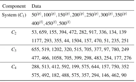
Table 2.2: Weapon system surveillance data. (Data are in hours. Data with superscript (p for pass) are right-censored observations where the unit worked at the time tested. Data with superscript (f for fail) are left-censored observations where the unit failed at the time tested.)
Component Data System (C1) 50(p),100(p),150(p),200(p),250(p),300(p),350(p) 400(f),450(f),500(f) C2 53, 659, 155, 394, 472, 282, 917, 336, 134, 139 1177, 293, 355, 44, 1504, 157, 470, 51, 235, 251 C3 655, 519, 1202, 320, 515, 705, 377, 97, 780, 249 477, 466, 1058, 705, 399, 298, 483, 254, 177, 276 C4 288, 513, 412, 592, 199, 575, 644, 157, 750, 352 575, 492, 182, 488, 575, 357, 294, 146, 462, 90
In this application, we use a Weibull distribution to model the component lifetimes. Our parameter-ization of the Weibull density for lifetimes for componentCi,i=1,2,3, is
fi(t|ψi,λi) = ψi λi (t/λi)ψi−1exp −(t/λi)ψi ,
so thatΘi= (ψi,λi). And the reliability function for this parameterization isRi(t|ψi,λi) =exp[−(t/λi)ψi].
We assume a hierarchical prior for the ψi andλi, with theψi and λi conditionally independent with
Gamma distributions given(aψ,bψ)and(aλ,bλ), respectively. That is, π(ψi|aψ,bψ) = baψ ψ Γ(aψ) ψiaψ−1exp −bψψi , π(λi|aλ,bλ) = baλ λ Γ(aλ) λaλ−1 i exp(−bλλi).
To complete the hierarchical specification, we assume thataψ,bψ,aλ,bλhave independent prior Gamma distributions with diffuse prior distributions; diffuse prior distributions reflect that little if any prior knowledge and allow the results to be driven by the data. This last layer of hierarchy is chosen for convenience and the parameter values are chosen so that the prior variance for these parameters is ap-proximately 10,000. There is little additional information to inform this choice. In other examples,
the choice of the hyperparameters may be guided by historical data or engineering judgement, although interpretation at the hyperparameter level may be increasingly difficult as the number of levels increases (as is the case with most hierarchical models).
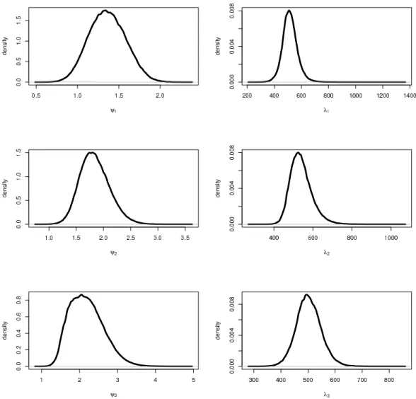
We used the MH algorithm to obtain draws from the joint posterior distribution as discussed in the preceding section. The posterior distributions that are presented below were based on 1,000,000 draws from the joint posterior distribution. The posterior distribution for each parameter governing the data likelihood is plotted in Figure2.2. Of interest in reliability assessments is the probability that a particular component exhibits increasing or decreasing failure rates (IFR or DFR). The posterior probability that each component has an increasing failure rate can be computed from the marginal distribution ofψi, by
computing thePr(ψi>1|D). The probability thatC1has an increasing failure rate is 0.947, whileC2
andC3have probabilities of an increasing failure rate that exceed 0.999. The reliability functions of the
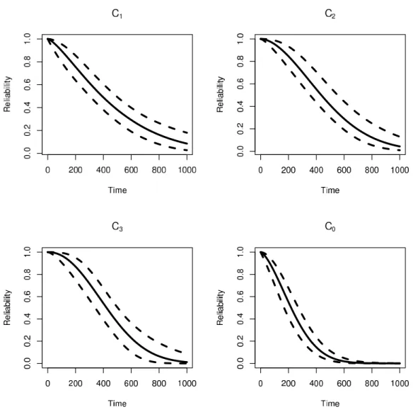
system and components are plotted in Figure2.3.
As with any system reliability assessment, our primary endpoints of interest are the component and system reliabilities. In Table2.3, we present the posterior central credible intervals (C.I.) for the two primary endpoints, 200 hours and 300 hours.
Table 2.3: Posterior credible intervals (C.I.) on the reliability of each component and system at two primary endpoints, 200 and 300 Hours.
Component Time 95% Central C.I.
System (C0) 200 (0.41,0.68) System (C0) 300 (0.20,0.44) C1 200 (0.63,0.85) C1 300 (0.49,0.73) C2 200 (0.75,0.94) C2 300 (0.59,0.84) C3 200 (0.75,0.95) C3 300 (0.57,0.84)
Our model for system reliability is relatively complex and contains a number of assumptions that should be verified. The primary concern in the full system reliability model proposed here is whether
Figure 2.2: Marginal posterior distributions of the parameters governing the component Weibull like-lihood Contributions. (The left panel are the posterior distributions forψ’s and the right panel are the posterior distributions forλ’s.)
the model adequately represents the data at subsystem and full system levels. As such, we restrict attention to the global model diagnostic proposed in Johnson (2004). This diagnostic can be considered as a Bayesian version of Pearson’s chi-squared goodness-of-fit test.
The diagnostic requires the observations to be conditionally independent given the value of the parameter vector Θ, which they are in our application. Let ˜Θdenote a single value of the parameter
Figure 2.3: Reliability distributions as a function of time in hours. (The solid line is the posterior median and the dashed lines are the 95% central credible interval.)
vector drawn from the posterior distribution, and letuj, j=1, . . . ,n, be defined as
uj= F(yj|Θ˜) if failure observed,
Uniform(0,1)F(yj|Θ˜) if left censored,
F(yj|Θ˜) +Uniform(0,1)(1−F(yj|Θ˜)) if right censored,
where Uniform(0,1)is a random draw from a uniform random variable on (0,1). Then from results in Johnson (2004), it follows that the distribution of the chi-squared statistic obtained by assuming that the values of uj are drawn from a uniform distribution on (0,1) has a chi-squared distribution with
adjustment to the degrees of freedom need be made to account for the dimension ofΘ.
To apply this procedure to our model for the weapon system data (all left- or right-censored data), we chose five equiprobable bins and calculated 10,000 chi-squared statistics based on 10,000 posterior draws of ˜Θ. 12.3% of these values exceeded the 0.95 quantile of a chi-squared distribution on 4 degrees
of freedom, suggesting some lack of model fit based on this global diagnostic. We further assessed goodness-of-fit by applying the Bayesian chi-squared to each of the components (all failures observed) and found that only 1.7% of the Bayesian chi-squared statistics for component 1 exceeded the 0.95 quantile of a chi-squared distribution with 4 degrees of freedom. Furthermore, only 3.43% and 1.6% of the Bayesian chi-squared statistics for components 2 and 3 exceeded the limit. This gives confidence that the global model and the components all exhibit reasonable fits.
One issue commonly encountered in complex system reliability which is not addressed completely by the goodness-of-fit analysis above is model misspecification. A common pitfall in complex systems analysis is failure to recognize a failure mechanism. This results inmodel misspecification resulting
from an inaccurate portrayal of the system structure. Our proposed approach does not remedy this
problem. In fact, because our system level data are modeled using substitution at the component level, our approach relies more on an accurate representation of the system structure. To develop our represen-tation of the system, we use approaches like those discussed in Anderson-Cook (2009), which checks the appropriateness of series and parallel structures, and Graves et al. (2010), which adds discrepancy terms to account for differences between the component and higher-level data.
2.4 Example: More Complex System in Fault Tree
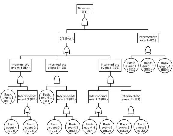
Consider the fault tree shown in Figure2.4. This particular system structure has been analyzed by several authors (Russell et al. 1994a,b; Hamada et al. 2004; Graves et al. 2007), although never with lifetime data at the components and system. Data for the example are given in Table2.4.
The fault tree representation attributes an event for the system (top event) to events of lower levels (subsystems and components) using logical gates. In our system reliability context, we are usually interested in the event of system failure. We call those events requiring no further decompositionbasic
occurred is calledintermediate event. For more details about fault tree, see for instance Vesely et al. (1981).
Figure 2.4: More complex fault tree example
2.4.1 Likelihood
For basic events 1, 2, and 4, we use a Weibull distribution to model their lifetime data, respectively, with the same parameterization as in the example in Section2.3. That is, fori=1,2,4,
fi(t|ψi,λi) = ψi λi (t/λi)ψi−1exp −(t/λi)ψi .
We assume that the lifetimes of basic events 3 and 5 are dependent. We model their joint distribu-tion using the absolutely continuous bivariate exponential (ACBVE) distribudistribu-tion from Block and Basu (1974). This distribution is often used to model a pair events which are positively correlated and have negligible probability of simultaneous failures. The bivariate distribution of(Ti,Tj)∼ACBVE(δ1,δ2,δ12)
Table 2.4: Lifetime data (years) for the more complex system and its components. The sample sizes for BE1, BE2, BE3 and BE5 (jointly), BE4, and TE are 20, 30, 25, 20, and 20, respectively.
Component Data BE1 17.2, 10.85, 33.7, 55.55, 52.85, 11.93, 39.5, 9.21, 55.14, 26.68, 52.42, 30.85, 31.27, 14.85, 29.87, 43.51, 46.44, 58.67, 63.11, 28.45 BE2 25.21, 32.94, 67.63, 57.32, 13.09, 91.16, 44.57, 46.11, 38.18, 40.49, 51.65, 48.11, 36.09, 28.44, 33.53, 30.39, 67.59, 35.63, 60.63, 68.83, 34.57, 76.65, 42.33, 30.63, 48.27, 64.76, 49.56, 50.87, 31.67, 45.61
BE3 & BE5 (4.3, 14.93), (22.66, 24.82), (6.51, 33.03), (4.29, 72.78), (12.03,
1.39), (98.72, 84.47), (16.81, 13.32), (14.69, 13.28), (21.44, 27.04), (11.13, 8.85), (52.74, 40.76), (6.15, 0.91), (4.9, 4.09), (5.87, 6.86), (33.03, 44.29), (5.09, 5.86), (37.32, 41.53), (5.27, 21.02), (1.75, 19.61), (28.02, 24.47), (27.84, 38), (123.61, 5.4), (33.83, 23.22), (25.58, 36.66), (8.31, 8.43) BE4 43.58, 10.7, 64.73, 7.25, 47.58, 13.24, 26.88, 8.7, 28.04, 5.62, 16.48, 16.46, 21.07, 41.98, 29, 53.44, 6.8, 96.83, 1.45, 30.52, System (TE) 7.14, 39.64, 29.86, 15.16, 30.13, 41.62, 42.97, 14.05, 45.6, 47.07, 29.8, 17.24, 6.5, 16.17, 25.69, 53.02, 45.97, 16.04, 7.53, 39.03
(δ1>0,δ2>0,δ12>0) has the following probability density function:
f(ti,tj|δ1,δ2,δ12) = δ1δ(δ2+δ12) δ1+δ2 exp(−δ1ti−(δ2+δ12)tj) if 0<ti<tj, δ2δ(δ1+δ12) δ1+δ2 exp(−δ2tj−(δ1+δ12)ti) ifti>tj>0, whereδ =δ1+δ2+δ12. In addition, the joint reliability function for the ACBVE is
R(ti,tj|δ1,δ2,δ12) =δ/(δ1+δ2)exp −δ1ti−δ2tj−δ12ti∨tj −δ12/(δ1+δ2)exp −δti∨tj , wherex∨y=max(x,y).
A property of the ACBVE distribution is that if (X,Y) =ACBVE(δ1,δ2,δ12), Z=min(X,Y)has
exponential distribution with parameterδ =δ1+δ2+δ12. That is,
The probability that the system is working (the reliability function) is
RT E(t) =R1(t)R3(t) +R1(t)R2(t)R4(t) +R2(t)R3(t)R4(t)
−2R1(t)R2(t)R3(t)R4(t) +R1(t)R5(t)−R1(t)R35(t) (2.5)
+R2(t)R4(t)R5(t)−2R1(t)R2(t)R4(t)R5(t)
−R2(t)R35(t)R4(t) +2R1(t)R2(t)R35(t)R4(t),
whereR35(t)is the reliability function of min(T3,T5). Additional details of the derivation of the system
reliability for general cases can be found in Hamada et al. (2008). We derive the density function of the lifetime distribution for the system (TE) as follows.
Let fi(t) (i=1,2,3,4,5,35)denote the lifetime distribution of componentiand f35(t)the lifetime
distribution of min(T3,T5). We know that fi(t) =−d Ri(t)
dt . Using Equation (2.5), the probability density
function for the lifetime of the system (TE) is:
fT E(t) =− dRT E(t) dt =f1(t)R3(t) +R1(t)f3(t) +f1(t)R2(t)R4(t) +R1(t)f2(t)R4(t) +R1(t)R2(t)f4(t) +f2(t)R3(t)R4(t) +R2(t)f3(t)R4(t) +R2(t)R3(t)f4(t) −2f1(t)R2(t)R3(t)R4(t) +R1(t)f2(t)R3(t)R4(t)+ R1(t)R2(t)f3(t)R4(t) +R1(t)R2(t)R3(t)f4(t) +f1(t)R5(t) +R1(t)f5(t)− f1(t)R35(t) +R1(t)f35(t) +f2(t)R4(t)R5(t) +R2(t)f4(t)R5(t) +R2(t)R4(t)f5(t) −2 f1(t)R2(t)R4(t)R5(t) +R1(t)f2(t)R4(t)R5(t)+ R1(t)R2(t)f4(t)R5(t) +R1(t)R2(t)R4(t)f5(t) − f2(t)R35(t)R4(t) +R2(t)f35(t)R4(t) +R2(t)R35(t)f4(t) +2f1(t)R2(t)R35(t)R4(t) +R1(t)f2(t)R35(t)R4(t)+ R1(t)R2(t)f35(t)R4(t) +R1(t)R2(t)R35(t)f4(t) .
2.4.2 Prior Distribution
We need to specify prior distributions for the parameters ψi, λi, δ1, δ2, and δ12. The priors are
summarized in Table2.5.
Table 2.5: Priors forψi,λi (i=1,2,4)andδ1,δ2, andδ12
Parameter Prior ψ1,ψ2,ψ4 Inverse-Gamma(3,2) λ1 Gamma(100,1/0.4) λ2 Gamma(100,1/0.55) λ4 Gamma(100,1/0.3) δ1,δ2,δ12 δ ≡δ1+δ2+δ12∼Inverse-Gamma(3,0.2) (δ1/δ,δ2/δ,δ12/δ)|δ ∼Dirichlet(1,1,1).
The prior distributions for ψ1,ψ2,ψ4 are independent Inverse-Gamma(3,2) with both mean and
variance being 1. Sinceψidetermines whether the hazard rate is increasing (ψi>1), decreasing (ψi<
1), or constant (ψi=1) for the Weibull distribution, an Inverse-Gamma distribution with mean 1 and
variance 1 is relatively diffuse for theψi. The specifications forλi’s are independent, informative, and
represent expert judgement about the components.
For the parametersδ1,δ2, andδ12of the ACBVE for basic events 3 and 5, we specify
δ1+δ2+δ12∼Inverse-Gamma(αδ,βδ),
so that the mean and variance areβδ/(αδ−1)andβδ2/ (αδ−1)2(αδ−2)respectively. Our rationale is that the minimum of lifetime of basic events 3 and 5, for which we might have some prior information in practice, has an exponential distribution with mean(δ1+δ2+δ12)−1. Further, givenδ =δ1+δ2+δ12,
we specify
δ1/δ,δ2/δ,δ12/δ
|δ∼Dirichlet(a1,a2,a12).
Then the joint prior distribution forδ1,δ2,δ12is
Suppose that we have additional independent prior information about the lifetime of the system. In particular, we have expert opinion that the distribution of system reliability at age 30 years is a Beta(15,15). We would like to incorporate this information; however, our likelihood is specified in terms of the lifetime distributions of the basic events. Consequently, we need to combine the information about the system with the prior information specified in Table2.5.
To combine the prior information, we use Bayesian melding, as discussed in Poole and Raftery
(2000). The system reliability at a specific timet∗, denoted byRT E(t∗), is given in Equation (2.5). The
prior distributions specified in Table2.5induce a prior distribution onRT E(t∗)through Equation (2.5).
For brevity, denote(ψ1,ψ2,ψ4,λ1,λ2,λ4,δ1,δ2,δ12)byθandRT E(t∗) =M(θ).
Denote the prior distribution specified onθbyq1(θ); the induced prior onM(θ)byq∗1(M(θ)); and the prior onM(θ)byq2(M(θ)). The melded prior forθ is given by
π(θ)∝q1(θ)
q2 M(θ) q∗1 M(θ)
!1−α
. (2.6)
For this exampleM(θ) =RT E(t∗=30);q1(θ) =q1(ψ1,ψ2,ψ4,λ1,λ2,λ4,δ1,δ2,δ12), i.e., the joint
prior probability density function as specified in Table2.5. The probability density function forq2(·)is
q2(M(θ))∝M(θ)14(1−M(θ))14.
The probability density function forq∗1(·)is obtained by simulation: generate samples fromq1(θ)and evaluateM(θ)at these values. Sinceq∗1(M(θ))does not have a simple parametric form, we estimate it using nonparametric (specifically, kernel density) methods. For this example, following Poole and Raftery (2000), we setα =0.5.
2.4.3 Posterior Distribution
Given the specified likelihood and prior distribution, we use MCMC to draw samples from the posterior distribution. After deriving the likelihood for the system-level data, the primary computational difficulty comes in the evaluation of the prior distribution given in Equation (2.6). The induced prior, q∗1(M(θ)) does not have a simple parametric form; since it must be repeatedly evaluated during the evaluation of the posterior density in the MCMC algorithm we tabulate the induced prior distribution at 106values between 0 and 1. When we want to evaluate theq∗1(M(θ)), we use the tabulated value closest
toM(θ∗). In our implementation, the induced prior was computed by the built-in functiondensityin R, and the Metropolis algorithm was implemented inCwith The GNU Scientific Library (Galassi et al. 2009).
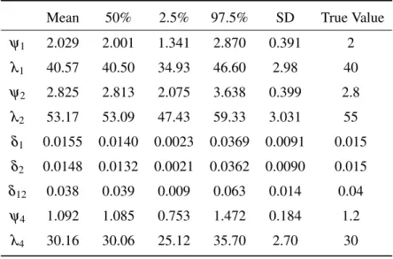
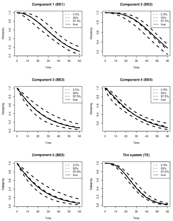
Table2.6summarizes the quantiles of the marginal distribution of the parameters. Figure2.5depicts the estimated reliability function with time for the basic events and the system (TE).
Table 2.6: Empirical mean, median, 2.5% and 97.5% quantiles, and standard deviation for each model parameter
Mean 50% 2.5% 97.5% SD True Value
ψ1 2.029 2.001 1.341 2.870 0.391 2 λ1 40.57 40.50 34.93 46.60 2.98 40 ψ2 2.825 2.813 2.075 3.638 0.399 2.8 λ2 53.17 53.09 47.43 59.33 3.031 55 δ1 0.0155 0.0140 0.0023 0.0369 0.0091 0.015 δ2 0.0148 0.0132 0.0021 0.0362 0.0090 0.015 δ12 0.038 0.039 0.009 0.063 0.014 0.04 ψ4 1.092 1.085 0.753 1.472 0.184 1.2 λ4 30.16 30.06 25.12 35.70 2.70 30 2.5 Conclusions
Our Bayesian model for system reliability offers several advantages over other existing models for system reliability. Among these are the ease of including diverse sources of information at different levels of the system in the model for overall system reliabilities, a coherent framework for incorpo-rating multiple sources of prior expert opinion, and the natural elimination of aggregation errors (Bier 1994) through the definition of non-terminal node reliabilities using the assumed structure of the system reliability block diagram and terminal node lifetime distributions.
In the setting where there are few, or perhaps no, system tests available, the borrowing of strength across nodes allows decision makers to use existing data in a more efficient manner. The hierarchical specification that we discuss in the first example allows the incorporation of less specific prior
informa-Figure 2.5: Reliability distributions as a function of time (in years). (The dashed lines are the posterior median and the 95% central credible interval. The solid line is the true reliability function.)
tion based on groupings of component nodes with similar reliabilities, rather than more specific speci-fications. This reliance on elicited priors is thereby shifted more to structural similarity of components and observed data. Johnson et al. (2003) also discussed the benefits of such hierarchical specifications. As the complexity of the system increases, the primary challenges arise in three areas. The first is in
model development and checking. The development of models that capture the interactions in complex systems is a detailed and time-consuming task (see, for example, Wilson et al. 2007). Further, spe-cialized diagnostics for model checking within a complex system model remain to be developed. The second challenge arises from the increasing complexity of the likelihood, although the use of structure functions and software for finding cut sets can help here. The third challenge arises from the increased computation times required for large systems. However, we have not found that new specialized algo-rithms are required for our computations.
CHAPTER 3. BAYESIAN METHODS FOR ESTIMATING THE RELIABILITY OF COMPLEX SYSTEMS USING HETEROGENEOUS MULTILEVEL INFORMATION
3.1 Introduction
In the preceding chapter, we study the reliability over time for systems with multilevel lifetime data and priors in a Bayesian framework. However, there are more general situations where we have heterogeneous information for assessing system reliability. For example, in addition to lifetime data, we might also have pass/fail data and degradation data. Generalizing previous work (Johnson et al. 2003; Wilson et al. 2006) and the preceding chapter, we discuss models for pass/fail, lifetime, degradation, and expert opinion data at any system level.
To provide context, we review some research particularly relevant to addressing pass/fail data, life-time data, and degradation in system reliability research. Considering only pass/fail data, Mastran (1976); Mastran and Singpurwalla (1978) described a procedure to approximate the posterior mean re-liability of a coherent system using test and prior data at both the component and system level. Martz et al. (1988); Martz and Waller (1990) proposed a bottom-up approach for approximating the posterior distribution of reliability of series and parallel systems of independent Binomial subsystems and com-ponents. Tang et al. (1997) proposed methods to obtain the exact posterior distributions in special cases. Johnson et al. (2003) developed full simultaneous Bayesian for pass/fail data collected at any level of the system.
Extending beyond pass/fail data, Thompson and Chang (1975) and Chang and Thompson (1976) considered first the reliability of subsystems with one or more components in series, where each com-ponent has an independent excom-ponential distribution, and then compute Bayesian credible intervals for arbitrary series-parallel system composed of these subsystems. Winterbottom (1984) surveyed classical and Bayesian results for estimating system reliability from Binomial and exponential component data
in coherent systems. Robinson and Dietrich (1988) considered component-level data with exponential lifetimes that have decreasing failure rates as the system develops. Sharma and Bhutani (1994a) esti-mated the availability of series and parallel systems where the components have exponential time to failure and repair. Bergman and Ringi (1997a) considered dependence between components induced by common operating environments; Bergman and Ringi (1997b) used data from non-identical envi-ronments. Hulting and Robinson (1994) is an exception to the above approaches, as they generalize the results of Martz et al. (1988) to make approximate inferences about the reliability of the system using multi-level information. They approximate the reliability for a series system using non-homogeneous Poisson processes to model the repair histories of repairable subsystems and time-to-failure data (mod-eled with a Weibull distribution) for nonrepairable subsystems.
Markov chain Monte Carlo (MCMC) has made fully Bayesian methods possible for addressing system reliability problems; for example, Johnson et al. (2003) and Hamada et al. (2004) proposed fully Bayesian approaches for simultaneously estimating the reliability for a system and its subsys-tems/components described by a fault tree using pass/fail data. Wilson and Huzurbazar (2007) consid-ered a system represented as a Bayesian network (BN), also with pass/fail data. Wilson et al. (2006) and Hamada et al. (2008) proposed approaches for assessing system reliability with pass/fail data at the system, and pass/fail, lifetime, or degradation data at the components.
This chapter discusses a unified fully Bayesian approach for simultaneously estimating system, subsystem, and component reliability when there are pass/fail, lifetime, degradation, or expert judgment data at any level of the system. We develop this methodology using the three components system with the same logic structure as in Chapter2. We represent this system in a fault tree in Figure3.1, equivalent to the reliability block diagram in Figure2.1. In Section3.2, we introduce the models. In Section3.3, we demonstrate the methodology by considering three scenarios applied to Figure3.1. In each scenario, one component has pass/fail data collected over time, one has lifetime data, and one has degradation data; Scenario 1 has pass/fail data collected over time at the system, Scenario 2 has lifetime data at the system, and Scenario 3 has degradation data at the system. In particular, we reanalyze Scenario 1 with incorporating some other prior information from the system level. In Section3.4, we discuss extensions of the methodology.
Figure 3.1: Three-component series system
3.2 Model Specification
In our development, we assume a coherent system represented as a fault tree. The fault tree describes the relationships between different levels of failure events (top event, basic event, and intermediate event) in our system reliability context. For details regarding fault tree, see Section2.4of Chapter2. In this chapter, we simply divide events intobasic eventsandnon-basic eventsas we treat them differently during modeling.
In Figure3.1, we label each event withCi(i=0,1,2,3). In particular,C0denotes the system (a
non-basic event) andC1,C2,C3denote the three components (basic events). For any eventCi, letRi(t|Θi)
denote its reliability function at timetgiven parametersΘi. LetTi be the random variable associated
with the lifetime ofCi, with probability density function fi(t|Θi)and cumulative distribution function
Fi(t|Θi). We assume thatRi(t|Θi)is differentiable with respect totandΘi.
By definition, we have the following relations:
Ri(t|Θi) =Pr{Ti>t|Θi}=1−Fi(t|Θi), and fi(t|Θi) = dFi(t|Θi) dt = d 1−Ri(t|Θi) dt =− dRi(t|Θi) dt . (3.1)
As a result, forCi, eitherRi(t|Θi)or fi(t|Θi)is sufficient to determine the other. We call the lifetime
The first step of model development is specifying the reliability functionRi(t|Θi), which is specified
directly or induced from the probability density function fi(t|Θi). The second step is to use the system
structure to determine the reliability functions for all of the non-basic events. Lifetime distributions for each event follow from the reliability functions. If the non-basic events have lifetime or pass/fail data, their likelihood functions are straightforward. If there are degradation data observed for the non-basic events, we specify the likelihoods with constraints determined by their reliability functions. Finally, the data for all events can be combined to model the system and estimate reliabilities.
For example, consider the system in Figure 3.1. The first step, modeling the three basic events, is detailed in Section 3.3. In the second step, since the system works if and only if all three com-ponents work, the reliability function of system is the product of the reliability functions of the three components. That is,
R0(t|Θ0) =R1(t|Θ1)·R2(t|Θ2)·R3(t|Θ3). (3.2)
Another example of expressing the reliability of a system/subsystems in terms of basic events concerns the system in Figure3.2. By virtue of the system structure, we can obtain the reliability functions of non-basic events as follows (parametersΘi’s are suppressed):
R4(t) =1−(1−R2(t))(1−R3(t)) =R2(t) +R3(t)−R2(t)R3(t), R0(t) =R1(t)R4(t) =R1(t)R2(t) +R1(t)R3(t)−R1(t)R2(t)R3(t).
3.2.1 Pass/fail Data
Suppose at time si j (j=1, . . . ,ni),Ni j tests have been conducted onCi, withbi j passing the test.
Denote the data vector asbi. The likelihood function for a basic event, using the Binomial distribution is given as Li(bi|Θi) = ni
∏
j=1 Ni j bi j Ri(si j|Θi) bi j 1−Ri(si j|Θi) Ni j−bi j . (3.3)The reliability function in Equation (3.3) can take many forms. Consider, for example, a logit model, where we specify the reliability function as
Figure 3.2: Another fault tree system:C4works if at least one ofC2andC3works; the systemC0works
if and only if bothC1andC4work.
where logit−1is the inverse of logit function which is defined as logit(x) =logx−log(1−x),0<x<1. The reliability functionRi(t)for a non-basic event is determined by the system structure. In
partic-ular,Ri(t)is a function of the reliabilities of basic events as illustrated by Equation (3.2) for the system
in Figure3.1.
3.2.2 Lifetime Data
For lifetime data, letti=ti1,ti2, . . . ,timi be the lifetime data collected for eventCi. Assume the data
are independent and identically distributed, with likelihood
Li(ti|Θi) = mi
∏
j=1
fi(ti j|Θi). (3.4)
The likelihood is easy to generalize to censored data, with details given in Section3.4.
The probability density function fi(t) for a basic event depends on which model is used. As for
a non-basic event, the density function can be derived from its reliability function. For the system in Figure3.1, by using the relationship of Equation (3.1), the density function for the lifetime ofC0can be
3.2.3 Degradation Data
Degradation data measure some quantity about a component or subsystem that is indirectly related to reliability. In particular, degradation data are typically thought of a continuous quantity that changes over time, with failure occurring when the quantity passes some threshold.
Consider degradation data for eventCi, and suppose that we have measured a total ofvi different
units. Denote the time of the measurements,di jk, asqi jk, where j=1, . . . ,vi andk=1, . . . ,zi j. That
is, for each of thevi units, we measure the degradation quantityzi j times. LetDi jk denote the random
variables associated with the degradation quantitiesdi jk.
For basic events, the reliability function is derived from the degradation model: specifically, the reliability is the probability that the degradation quantity is above the threshold at timet. For example, consider the degradation process as specified in Wilson et al. (2006):
Di jk∼Normal(αi−βi j−1qi jk,σi2), αi>0,βi j>0,σi>0. (3.5)
That is, all events are identical att=0, but they each degrade at their own rates. Letdi denote the degradation data forCi. We can construct a likelihood function using Equation (3.5):
Li(di|βi,αi,σi) = vi
∏
j=1 zi j∏
k=1 1 σi φ di jk−αi+βi j−1qi jk σi ! , (3.6)whereφ(·)is the probability density function of standard normal distribution.
To connect the degradation model with the lifetime distribution and reliability function, let τi be
the threshold of the degradation process. This event fails when the degradation quantity is less thanτi.
Then we have
Ti j=inf{t≥0 :αi−βi j−1t≤τi}= (αi−τi)βi j, αi>τi>0. (3.7)
Suppose that we further assume that logβi j ∼Normal(µi,ψi2). Then the lifetime of the event has
a Log-normal distribution. That is, logTi j ∼Normal(µi+log(αi−τi),ψi2). As a result, the reliability
function at timetis Ri(t|Θi) =1−Φ logt−µi−log(αi−τi) ψi , Θi= (µi,ψi,αi,τi,σi),
For non-basic events, we first derive the induced lifetime distribution as described in Section3.2. If we further assume the same degradation model as Equation (3.5), the distribution of (αi−τi)βi j
in Equation (3.7) is determined for the non-basic event. In our Bayesian model, we must choose our prior distribution for (αi, τi, βi j) such that the distribution of(αi−τi)βi j is the same as the induced
lifetime distribution for eventCi. One simple way to achieve this is to specify the following conditional
probability density distribution function forβi j in terms of the induced lifetime distribution fi(t|Θi):
gi(βi j|Θi) = (αi−τi)fi
βi j(αi−τi)|Θi
. (3.8)
This specification forβi j, along with any proper prior distributions forαiandτi, makes the distribution
of(αi−τi)βi j coincide with the induced lifetime distribution. Consequently the likelihood function for
a non-basic event according to the above model specification still has the form of Equation (3.6), but with constraints onβi jfrom lower-level events.
3.2.4 Prior Information
Specifying prior distributions in a Bayesian context is also part of the modeling process. An advan-tage of Bayesian methodology is that we can incorporate “non-data” information into our models; for example, information from expert opinions, historical data, and from similar systems.
Initial specification of prior distributions for the parameters describing basic events follows standard Bayesian practice. However, some thought must be given to the specification of prior distributions for the degradation data. Suppose that we are working with the model Equation (3.5). Consider the specification of the priors for the degradation quantity at time 0,αiand the thresholdτi, both of which
are assumed to be positive. We consider two approaches.
A first approach, which is mentioned in Wilson et al. (2006), is to specify a Gamma prior distribution onαi and then Beta distribution onτi/αi givenαi. This approach is useful if we want to impose
non-informative priors onτior on bothαiandτi.
As an example, suppose that we specify the following Gamma prior distribution onαiand uniform
distribution onτi/αi givenαi:
(Note that our Gamma distribution has a parameterization such that the above specification forαi has
meanναi·ξαi.)
We may have detailed information about the thresholdτithat leads us to specify an informative prior
forτi. This can be difficult to specify using the preceding approach. However, consider the following.
We specify an informative prior for τi and then a conditional prior distribution for αi given τi. An
example using Gamma distribution is given as follows:
τi∼Gamma(ντi,ξτi); (αi−τi)|τi∼Gamma(ναi−τi,ξαi−τi).
Specifying prior distributions for non-basic events requires additional thought. Recall that the re-liability and lifetime of non-basic events are functions of the parameters of the basic events, and the degradation model has constraints from lower level events. This implies that for non-basic events, we need to specify prior distributions on functions of parameters. In addition, the prior distributions specified on the parameters of basic eventsinduceprior distributions on the reliability and lifetime of non-basic events. Consequently, if we also have prior information about the reliability or lifetime of non-basic events, we need a way to combine the information.
We use the Bayesian melding approach proposed in Poole and Raftery (2000). Suppose that we
have independent prior distributions on parameters θ and φ =M(θ), specified by q1(θ) and q2(φ)
respectively. M(·)is a deterministic function. The prior onθ induces an additional prior onφ=M(θ), denoted byq∗1(φ).
Poole and Raftery (2000) proposes pooling q∗1(φ) andq2(�