V
OLATILITY IN THE
A
MERICAN
C
RUDE
O
IL
F
UTURES
M
ARKET
1 Delphine LAUTIER & Fabrice RIVACahier de recherche du C
EREGn° 2004-08
This draft : 10/10/2004
Delphine Lautier is Assistant Professor at the University Paris Dauphine. Postal Address: Cereg
University Paris Dauphine
Place du Maréchal de Lattre de Tassigny
75 775 Paris Cedex 16
Telephone number: 33 (1) 44 05 46 42 Fax : 33 (1) 44 05 40 23
Email: Delphine.Lautier@ dauphine.fr
Fabrice Riva is Assistant Professor at the University Paris-Dauphine. Postal Address: Cereg
University Paris Dauphine
Place du Maréchal de Lattre de Tassigny
75 775 Paris Cedex 16
Telephone number: 33 (1) 44 05 49 88 Fax : 33 (1) 44 05 40 23
Email: Fabrice.Riva @ dauphine.fr
VOLATILITY IN THE AMERICAN CRUDE OIL FUTURES MARKET
Delphine LAUTIER & Fabrice RIVA CEREG
University Paris-Dauphine
ABSTRACT. This article focuses on the impact of derivative markets on the American crude oil market.
More precisely, it analyses prices volatility. The latter is separated into two components: an information component, that reflects a rational assessment of the information arrival, and an error component, that represents the noise introduced by the trading processes. We show that there is a peak of volatility during the open outcry session and that this phenomenon is mainly due to the arrival of information. Thus, most of the price discovery process occurs during the exchange trading hours in the crude oil futures market. Moreover, there is some noise trading during the nights (electronic sessions) and during the week-end.
KEY WORDS: volatility – crude oil – noise trading – information – open outcry – electronic trading
This article aims at answering the following questions: does the existence of derivatives markets have an undesirable influence on the behaviour of the underlying commodities? Do the commodity markets become nowadays more volatile, more speculative than before? These questions gained in importance during the last decade, as a result of the intensified presence of certain categories of investors such as hedge funds. The untimely and heavy interventions of these actors could indeed have an impact on the prices. Whereas this problem is relevant for all markets, it is especially important for commodity markets, because in this context, the real and financial spheres are intimately associated.
The theoretical framework of our study is the microstructure of financial markets. Through the study of the determinants of volatility, it aims at examining the informational content of commodity futures prices. This could be a first step in a work aiming to appreciate the quality of the services
produced by the futures markets, namely the redistribution of risk between different categories of operators which are more or less risk averse, and the promotion of informative signals – the futures prices. Our method consists in decomposing volatility into two components: the first one is called fundamental volatility and comes from the physical market; the second one is the volatility caused by trading. On a practical point of view, the interest of this work is twofold. Firstly, it should give a way to better appreciate the efficiency of hedging strategies. Secondly, it is important for regulatory purposes.
The problem of volatility is especially important for energy markets, as they become more and more integrated. As a result of tightened cross market linkages, a shock induced by the traders can spread not only to the physical market but also to other energy markets. Among the different energy markets, we focused on the American crude oil futures market because it is nowadays the most developed commodity market. Thus, information on futures prices is abundant.
This article is organized as follows. Section 1 is devoted to the previous literature on the subject. Section 2 presents the data. Section 3 is centred on the determinants of volatility. Section 4 analyses the extent to which the open outcry session, the overnight electronic trading period and the week-end trading period affect the price process. Section 5 concludes.
SECTION 1. PREVIOUS LITERATURE
Literature on the impact of derivatives on commodity markets is relatively scarce. Among the available articles2, three different directions can be identified. The first one consists in directly investigating the influence of derivative markets. The second focuses on co-movements of commodity prices and spatial integration. The third examines the extent to which speculative trading could influence market prices and price informativeness.
Fleming and Ostdiek (1999) examine the effect of energy derivatives trading on the crude oil market between 1989 and 1997. They focus, first of all, on the introduction of new contracts on the market and their impact on volatility. They observe an abnormal volatility after the introduction of
crude oil futures. However, subsequent introductions of crude oil options and derivatives on other energy commodities seem to have no effect. Then the authors examine the influence of derivatives trading on the depth and liquidity of the market. Their analysis reveals a strong inverse relationship between the open interest in crude oil futures and spot market volatility. Specifically, when open interest is greater, the volatility shock associated with a given unexpected increase in volume is much smaller. This finding indicates that the futures market provides depth and liquidity to the crude oil market.
The influence of derivatives on the commodity markets was also examined through the such-called ‘herding phenomenon’. In 1990, Pindick and Rotenberg propose to define herding by a situation where traders are alternatively bullish or bearish on all commodities for no plausible economic reasons. According to these authors, herding is a possible explanation for the excess co-movement that they observe on the prices of seven different commodities. Pindick and Rotenberg show first of all that the prices of raw commodities have a persistent tendency to move together. They try to explain this co-movement by macro-economic variables: the expected inflation, the growth in industrial production, the consumer price index, several exchange rates, interest rates, money supply, and the S&P common stock index. However, they find that the co-movement is well in excess of anything that could be explained by these common variables, and they conclude that herding could explain this excess. Booth and Cinner (2001) extend this work. They analyse the linkage among agricultural commodity futures prices on the Tokyo Grain Exchange, and they suggest two explanations of long-term co-movements among the prices of agricultural futures contracts: common economic fundamentals or herd behaviour by market participants. Contrary to Pindick and Rotenberg, their results support the common economic fundamentals assumption.
Another way to deal with the subject of derivatives and their impact on commodity prices is to focus on the spatial integration of commodity prices. Indeed, integration can be seen as a way to reinforce the impact of a derivative market on underlying markets, through the linkages between cash markets. Spatial integration is most of the time examined through the methodology of co-integration and Granger causality tests.
Jumah, Karbuz and Rünstler (1999) study the spatial integration in the cocoa market, using prices extracted from London and New York markets. Interest rates are found to play a key role in establishing stationary long-run relationships. The authors also observe that futures prices Granger-cause spot prices, and that the reverse is not true. This is consistent with the view that futures prices adjust more quickly to new information compared to spot prices. Ewing and Harter (2000) study the co-movements of Alaska North Slope and UK Brent crude oil prices. Their results show that these oil markets share a long-run common trend, which suggests that the two markets are ‘unified’: there is price convergence in the markets. Kleit (2001) also examine the spatial integration of the crude oil markets. He studies seven types of crude oils. All of them are light crude oils, in order to reduce problems associated with quality differentials. His results show that oil markets are growing more unified. Milonas and Henker (2001) identify the variables that influence the relative price differentials of the Brent crude oil and the West Texas Intermediate. They show that the prices spreads are affected by convenience yields, which act as surrogates for demand/supply conditions and market price behaviour. Sanjuan and Gil (2001) study the spatial price relationship between European pork and lamb markets. The results indicate that markets for both commodities are integrated, not only in the long-run but in the short-run as well, although the price transmission process is more efficient in the pork meat industry.
All these works are important because spatial integration could exaggerate the possible negative influence of derivatives on the physical markets. However, they do not directly take into consideration the possible influence of derivatives.
The debate on the effects of derivatives trading is also closely related to the issue of the extent to which speculative trading could influence market prices and price informativeness. Several works have explored this field in the case of commodity markets. Foster (1995) shows that volume and volatility are contemporaneously correlated in the crude oil market. He suggests that both variables are influenced by the rate of information arrival. Moreover, he shows that the lagged volume explains prices variability, and concludes that the market is characterized by a certain degree of inefficiency. In 2000, Mossa and Silvapulle also present some evidence of a causal relationship between price and volume in the crude oil market. Using not only prices and volumes, but also open interest and prices
spreads, Girma and Mougoué, in 2002, confirm the results obtained by Foster in the crude oil market. Ciner (2002) finds similar results on the Japanese commodity markets. Thus, all these work conclude to a relative inefficiency of commodity markets, which might be due to the impact of derivatives markets by an effect of mimetic contagion.
Among all these different works, our study belongs to the third approach, the one centred on price informativeness. Three reasons lead us to work in this direction.
The first is the lack of reliable time series for the spot prices. Indeed, in most commodity markets, the spot price is regarded as a non observable variable because physical markets are geographically dispersed, transactions are not standardized, the prices reporting mechanism does not enforce the operators to disclose their transactions prices, etc. In the case of the United States crude oil market, spot prices are also affected by other problems specific to this market. The trading volume for the West Texas Intermediate grade, namely the underlying commodity of the futures contract, is very low and the spot prices only provide information for local supply and demand. Moreover, there are sometimes problems due to an under-capacity of the pipeline system, which can create prices jumps. The latter are due to the delivery system, no to general market conditions. This phenomenon, reported by Horsnell and Mabro (1993), is known as the “Cushing Cushion”, because usually difficulties arise at Cushing Oklahoma, which is the delivery point of the futures contract. Thus, it seems difficult, in the case of the American crude oil market, to deal directly with the relationship between spot and futures markets. Consequently, we focused our attention on the available information, namely the information relative to futures prices.
Our second choice was to renounce to study the impact of the introduction of futures contracts. This kind of event is indeed not so frequent, and we were more interested, at least in the first step of the study, in the behavior of specific operators and in the way derivatives markets could be used than in the impact of the presence of new instruments.
Our third choice consists in using the methods and concepts of microstructure. The latter were not extensively used in the case of commodities, probably because the quite recent availability of high frequency data on stock prices created a new field of researches and attracted a lot of attention. In commodity markets, the data are indeed not so abundant than they are elsewhere. However, there is
still work to be done with the available information. Indeed, whereas settlement prices, open interest and trading volumes have already been exploited, little or no attention has been paid, nowadays, to the information given by prices curve – the relationship between futures prices having different maturities – or by opening and closing prices. Yet, as we will see in the following study, they give precious indications on the volatility of futures markets.
SECTION 2. DATA AND DESCRIPTIVE STATISTICS
The data used for the study are related to the light, sweet crude oil futures contract of the New York Mercantile Exchange (Nymex). All have been operated such as the reconstituted time series always correspond to fixed monthly maturities. Indeed, the Nymex calendar was reconstructed in order to determine when a specific contract has, for example, a one- or a two-month maturity and to determine when the contract falls from the two-month to the one-month maturity. We collected daily futures prices, corresponding to the opening and settlement prices. For these time series, because of the lack of reliable data for opening prices, we had to retain only the first height maturities, even if there are actually very far delivery dates in the American crude oil futures market (until 7 years).
We extracted our data from Datastream, which leaded us to make certain choices. Indeed, when there was no information at a specific date and maturity, it was impossible to know whether this absence of information corresponds to a true missing value or to an absence of transaction. In order to render the data homogeneous, we decided to treat all zeros and missing values as missing values. Thus, we only consider that there is information when there is no missing value. Consequently, we can not take into account, as in Jones, Kaul and Lipson (1994) the fact that the absence of trading provides information.
Our sample period is 15 years long and ranges from January 1989 to December 2003. The choice of such a long period of time gives the possibility to examine the evolution of the market.
SECTION 3. THE VOLATILITY CAUSED BY TRADING
In this section, we first study the evolution of volatility, measured by the standard-error of prices changes, through time. This first overview will allow us to focus on some specific aspects of volatility and their evolution. More precisely, we will answer the following questions: does the trading process create a volatility in excess, which would not be observed in the absence of futures markets? Does this volatility change with the observation period?
3.1. The evolution of volatility during the observation period
Table 1 reproduces the volatility of the returns of settlement futures prices having a maturity between one and eight months, for each year of the observation period. The figures obtained offer a good illustration of the Samuelson effect3: the volatility of the returns strictly decreases with maturity. Indeed, the most important feature of the commodity prices curve’s dynamic is probably the difference between the price behaviour of nearby and deferred contracts. The movements in the prices of the prompt contracts are large and erratic, while the prices of long-term contracts are relatively still. This results in a decreasing pattern of volatilities along the prices curve.
Table 1. Standard-error of the returns, settlement futures prices, 1989-2003
Year 1 month 2 months 3 months 4 months 5 months 6 months 7 months 8 months
1989 0,0216 0,0167 0,0153 0,0145 0,0144 0,0138 0,0135 0,0133 1990 0,0384 0,0286 0,0260 0,0254 0,0247 0,0242 0,0239 0,0236 1991 0,0312 0,0298 0,0253 0,0226 0,0209 0,0197 0,0186 0,0175 1992 0,0127 0,0122 0,0114 0,0108 0,0103 0,0099 0,0096 0,0093 1993 0,0154 0,0137 0,0127 0,0120 0,0114 0,0108 0,0105 0,0102 1994 0,0182 0,0162 0,0147 0,0137 0,0130 0,0125 0,0121 0,0117 1995 0,0128 0,0109 0,0096 0,0088 0,0082 0,0077 0,0074 0,0071 1996 0,0261 0,0192 0,0175 0,0159 0,0148 0,0141 0,0137 0,0134 1997 0,0056 0,0036 0,0035 0,0036 0,0034 0,0035 0,0036 0,0037 1998 0,0297 0,0251 0,0222 0,0204 0,0189 0,0177 0,0168 0,0160 1999 0,0223 0,0205 0,0191 0,0180 0,0172 0,0165 0,0160 0,0155 2000 0,0273 0,0240 0,0220 0,0206 0,0197 0,0189 0,0183 0,0179 2001 0,0275 0,0253 0,0233 0,0220 0,0210 0,0201 0,0192 0,0185 2002 0,0213 0,0195 0,0182 0,0171 0,0163 0,0156 0,0150 0,0145 2003 0,0243 0,0216 0,0196 0,0182 0,0169 0,0158 0,0149 0,0142 Average 0,0223 0,0189 0,0171 0,0160 0,0152 0,0146 0,0141 0,0137
3 Samuelson (1965).
The 1st Gulf War (1990 and 1991) excepted, the years of high volatility correspond, for each maturity, to 1998, 1999, 2000, 2001, 2002 and 2003. Yet, all these years are located at the end of our sample period. Thus, there seems to be an increase in the volatility of the crude oil futures prices, at least since 1998, as depicted by Figure 1.
There are several possible explanations for the increase in volatility: it could be the result of the deregulation in the energy markets, or it could be a consequence of improved informational efficiency (markets with greater trading volume exhibit sometimes greater volatility).
Figure 1. Standard-error of the returns, settlement futures prices, 1989-2003 (ex 1990-1991)
0,0000 0,0050 0,0100 0,0150 0,0200 0,0250 0,0300 1989 1992 1993 1994 1995 1996 1997 1998 1999 2000 2001 2002 2003 1 month 2 months 3 months 4 months 5 months 6 months 7 months 8 months
Considering this increase in volatility, it is interesting to see if the phenomenon affects homogeneously all the maturities. Whenever it appeared that the short-term prices become relatively more volatile than the long-term prices, the rise in the volatility could be attributed to a rise in the volatility of the cash market. The latter would propagate in the paper market, and would be progressively absorbed, as maturity progresses, via the Samuelson effect.
Table 2. Differences between the volatility observed and the average of the period
Year 1 month 2 months 3 months 4 months 5 months 6 months 7 months 8 months
1998 0,0094 0,0075 0,0061 0,0054 0,0046 0,0041 0,0037 0,0033 1999 0,0019 0,0029 0,0030 0,0030 0,0029 0,0029 0,0029 0,0028 2000 0,0069 0,0064 0,0059 0,0056 0,0054 0,0053 0,0052 0,0052 2001 0,0072 0,0077 0,0072 0,0070 0,0067 0,0065 0,0061 0,0058 2002 0,0009 0,0020 0,0021 0,0021 0,0020 0,0020 0,0019 0,0018 2003 0,0040 0,0040 0,0035 0,0031 0,0027 0,0022 0,0018 0,0014
Table 2 illustrates, for each of the recent years, the impact of the volatility on the different maturities. It represents, indeed, for each year, the difference between the standard-error observed and the average calculated on the period (1990 and 1991 excepted). The results obtained show that the volatility of short-term prices rises more than the volatility of long-term prices in 1998, 2000, 2001, and 2003. For these years, the gap with the average volatility is all the more high than the expiration date of the contract is close. This observation indicates that the increase of the volatility of crude oil futures prices could be explained by a rise in the fluctuations in the underlying market.
3.2. The volatility caused by trading
One of the impacts of the presence of derivatives markets is that they can induce excess volatility, created by trading. In 1986, French and Roll proposed a method which allows estimating the impact of trading on volatility. Their framework is quite simple and intuitive. It relies on an empirical observation: prices are usually more volatile during trading hours than non trading hours. Two explanations can be found for this phenomenon: either it is due to the fact that the presence of a market gives the possibility to immediately reacting to news, or it is caused by pricing errors, which occur preferably during the trading session.
Once the phenomenon of higher volatility during trading hours has been observed, the objective of the analysis is to disentangle between these two possible sources of volatility: the information component, that reflects a rational assessment of the information arriving during the day, and the error component. The first part of the analysis is devoted to the identification of noise trading. Information on noise trading is obtained, first by examining the autocorrelation of daily returns – under the trading noise hypothesis, returns should be serially correlated – second, by comparing the variances computed on daily returns with variances for a longer holding period – such a comparison relies on the assumption that the importance of pricing errors diminishes as the holding period increases. The second part of the study consists in quantifying the impact of noise trading on the higher volatility recorded during trading hours.
This framework, originally conceived for the stock market, can be quite easily adapted to the crude oil futures market. The main differences between stocks prices and futures prices are twofold. First, there are no bid-ask spreads in the case of futures prices. Second, there are no such variables, in the futures markets, as the size of the firm or the market capitalization. Thus, the central element of the analysis is the maturity, and its influence on the behaviour of futures prices.
Since 1986, in the case of equities, information processing was further examined through the use of high frequency data. The frameworks were, most of the time, more sophisticated than the one proposed by French and Roll. However, intraday data are not publicly available in the case of the crude oil market, rendering this kind of analysis useless. Still, we have data that are more precise than those of French and Roll. Indeed, we can distinguish between opening and closing prices. This gives us the possibility to enlarge the analysis, and to give a deeper insight of the behaviour of prices, especially on the way they evolve during the day and the night.
The remaining of this section is organized as follows. First, we use different variance indicators to check whether the phenomenon of higher volatility during trading hours is also observed in the case of the crude oil market. Indeed, this empirical observation was left unexplored in the case of commodities. Then we identify the noise trading among the two possible sources of volatility. Lastly, we try to quantify the impact of noise trading on the volatility recorded during trading hours. 3.2.1. Volatility during trading and non trading hours
French and Roll consider three explanations for the phenomenon of higher volatility during trading hours: i) volatility is caused by public information which is more likely to arrive during normal business hours; ii) volatility is caused by private information which affects prices when informed investors trade; iii) volatility is caused by pricing errors that occur during trading. However, in this article, we will make no distinction between public and private information, because we only want to concentrate on the difference between the volatility caused by the reactions of the traders when there is an information arrival, and the volatility caused by pricing errors.
In order to investigate whether, in the case of the crude oil market, the volatility is higher during trading hours, we proceed in three steps. First, we compare trading, overnight and week-end variances. Second, we calculate ratios of trading over night variances and of trading over week-end
variances. Third, we normalize these indicators, so that the time span used for the computation of the variance is taken into account.
3.2.1.1. Trading, overnight and weekend variances
In this part of the study, we compare the volatility during the opening of the exchange, during the night, and during the weekend. On that purpose, we calculate different variance indicators, for each year and available maturity4 of our sample period. The first indicator is called trading variance and corresponds to the variance of returns from open to close. The second indicator, the overnight variance, corresponds to the variance of returns from close to open. The third indicator is the week-end variance, namely the variance of returns from Friday close to Monday open.
The first two indicators correspond to periods where trading is conducted via different forms. Trading variances reproduces the way prices fluctuates in open outcry trading, and overnight variances represent the changes recorded when trading is conducted via an internet based trading platform provided by the Nymex5. Compared with the preceding ones, week-end variances correspond to the period where the rate of information arrival is the most likely to be low. Indeed, the crude oil market being a worldwide market, information could a priori arrive during the open outcry session, as well as during the night. Figures 2 to 4 depict the evolution of these indicators over the whole sample period.
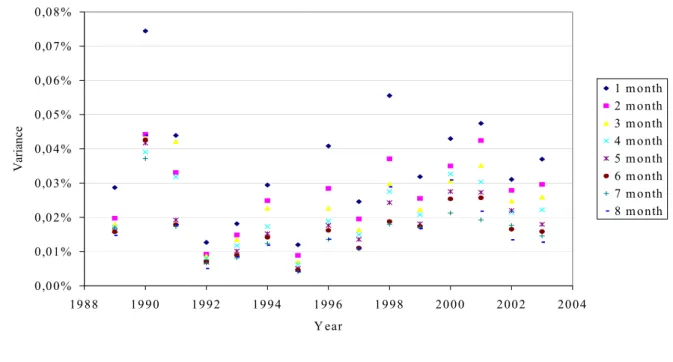
Figure 2. Trading variances
0,00% 0,01% 0,02% 0,03% 0,04% 0,05% 0,06% 0,07% 0,08% 1988 1990 1992 1994 1996 1998 2000 2002 2004 Y ear V ari an ce 1 m onth 2 m onth 3 m onth 4 m onth 5 m onth 6 m onth 7 m onth 8 m onth
4 The data relative on opening prices are far less abundant than those relative to settlement prices. Consequently, we worked only on the first height months.
5We do not have information concerning the proportion of the trading volume which is exchanged during the session of open
As was observed for the settlement prices, trading variances – the first Gulf War excepted – are higher in the second half of the period. Figure 2 also indicates that the one-month contract is always the most volatile, especially in the case of a crisis like the first Gulf War. Indeed, prices react as if the sole nearest month was absorbing the crisis. More generally, the trading variance of a given contract is inversely proportional to its maturity. Two combined effects can explain this phenomenon: the first is the Samuelson effect, which predicts that volatility is a decreasing function of maturity. The second is the trading volume, which is concentrated on the nearest maturities. Indeed, a rise in the trading frequency increases the level of noise that is impounded into prices.
Figure 3. Overnight variances
0,00 0,01 0,02 0,03 0,04 0,05 0,06 0,07 1988 1990 1992 1994 1996 1998 2000 2002 2004 Year Variance in% 1 month 2 months 3 months 4 months 5 months 6 months 7 months 8 months
Variances recorded during the night appear to be lower than trading variances. Two explanations could be invoked for this phenomenon. First, it could be due to the fact that, whereas the crude oil market is worldwide, information arrival is actually less intensive during the night – maybe because the market is concentrated in consumer areas. Second, it could be due to the fact that open outcry trading creates volatility in excess.
Figure 3 also show that variances exhibit a rise in volatility at the end of the period, and special peaks around the first Gulf War. However, some differences with the previous results can be underlined. Firstly, the peaks of volatility are not the same for the two indicators. The peak recorded in 1998 for the trading variance disappears when overnight variance is considered. And during the first
Gulf War, the peak of volatility does not correspond to 1990, but to 1991. Secondly, during periods of high volatility, the ordering of variances as a function of maturities can disappear, as is the case, for example, in 1991, in 1996 and in 2000.
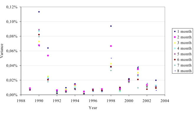
Compared with the former indicators, weekend variances, depicted by Figure 4, are characterized by huge jumps during periods of crisis: in that case, variances can reach from 3 to 6 times their normal level. More importantly, a probable consequence of the lack of volume during the weekend – mainly due, probably, to the absence of arbitragers and speculators – is that the hierarchy between contracts does not appear as clearly as before: the one-month contract is not necessarily the most volatile, except when a crisis occurs. Thus, the Samuelson effect disappears. The ordering of contracts becomes almost unpredictable – especially during low volatility periods – and the differences in volatility between the different maturities are quite low. During the week-ends, the shocks transmission along the prices curve becomes thus impossible.
Figure 4. Week-end variances
0,00% 0,02% 0,04% 0,06% 0,08% 0,10% 0,12% 1988 1990 1992 1994 1996 1998 2000 2002 2004 Year Var ianc e 1 month 2 month 3 month 4 month 5 month 6 month 7 month 8 month
Figure 2 to 4 show that both overnight and week-end variances are lower than trading variances. A simple indicator of the relative importance of these variances can be calculated: the ratio of overnight or week-end variances relative to trading variances.
3.2.1.2. Variance ratios
If hourly returns were constant across trading and non trading periods, the variance of weekend returns would be roughly 15 times the trading variance and the overnight variance would be roughly 5 times the trading variance6.
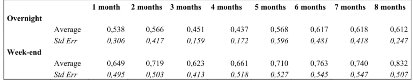
Table 3 reproduces the average variances ratios for each maturity during the whole sample period7. The results are consistent with those of French and Roll: the ratios are far less important than they should be, especially for the shorter maturities. They are lower for overnight variances than for week-end variances, which is normal. However, one could have expected a much higher difference between the two. This similarity leads to think, even if the information relative to volume during the night is not available, that overnight trading volume is quite low.
Table 3. Variance ratios, Overnight/Trading, and Week-end/Trading
1 month 2 months 3 months 4 months 5 months 6 months 7 months 8 months
Overnight Average 0,538 0,566 0,451 0,437 0,568 0,617 0,618 0,612 Std Err 0,306 0,417 0,159 0,172 0,596 0,481 0,418 0,247 Week-end Average 0,649 0,719 0,623 0,661 0,710 0,763 0,740 0,832 Std Err 0,495 0,503 0,413 0,518 0,527 0,545 0,547 0,507 3.2.1.3. Hourly variances
In order to give more insight on the relative importance of trading, overnight and week-end variances, these indicators must be normalized, so that the time span used for the computation of the variance is taken into account.
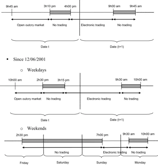
In order to compare trading and week-end variances on an hourly basis, we took into account the fact that, as illustrated by Figure 5, until December 2001, the trading session on the Nymex began at 9:45 am and ended at 3:10 pm, and that since December 2001, it begins at 10:00 am and ends at 2:30 pm. Thus, there are 5.42 trading hours during the first sub-period, and 4.5 during the second. Likewise, during the first sub-period, the week-end period ranges from Friday 3:10 pm to Monday
6As we will see later, the length of an outcry session is roughly 4 hours, namely 1/6° of a day. Thus, overnight trading is
conducted during 5/6° of a day, and the weekend as a length of 15/6°.
9:45 am, that is 66.58 hours8. During the second sub-period, it ranges from Friday 2:30 pm to Sunday 7:00 pm, due to the electronic system. This means that week-end variances do not exactly correspond to a period where there is absolutely no transaction. However, the period with no transaction, before electronic trading begins, represents 80% of the week-end’s length.
Figure 5. Trading sessions
From January 1997 to 11/06/2001
Since 12/06/2001 o Weekdays
o Weekends 10h00 am 2h30 pm
Open outcry market
9h30 am Electronic trading Date t 10h00 am No trading Date (t+1) 9h45 am 3h10 pm
Open outcry market
9h00 am Electronic trading Date t 9h45 am No trading Date (t+1) 4h00 pm No trading 3h15 pm No trading 2h30 pm
Friday Saturday Sunday Monday
7h00 pm 9h30 am 10h00 am
No trading Electronic trading
No trading
If we consider, as a first approximation, that returns are independent, then the variance must be strictly proportional to the length of time used for its calculation. As a result, we can normalize our variances on an hourly basis.
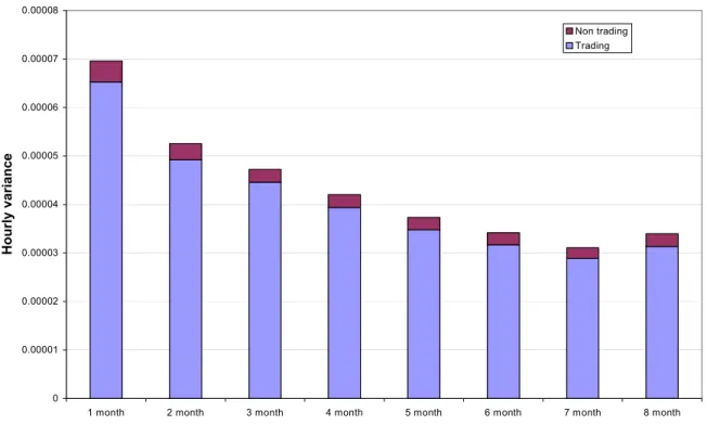
The results concerning trading and non trading (weekend) variances, on an hourly basis, are depicted on Figure 6. It shows that, on average on the whole period, the hourly trading variance is
8 As no information is currently available about the opening and closing hours prior to 1997, we will consider that those hours are valid from January 1989 to December 1996. .
much higher than the week-end variance. More precisely, the former is 15.25 times the latter. Moreover, the hourly variances clearly decrease with maturity and consequently with activity.
Figure 6. Trading and non trading (week-end) variances
0 0.00001 0.00002 0.00003 0.00004 0.00005 0.00006 0.00007 0.00008
1 month 2 month 3 month 4 month 5 month 6 month 7 month 8 month
Hourl
y vari
ance
Non trading Trading
The same kind of results are obtained comparing the trading and overnight hourly variances. More precisely, on average on the period, for all maturities, the former is 7.54 times the latter (the entire results, year by year and maturity by maturity, are provided by Appendix 2).
3.2.1.4. Conclusion on volatility during trading and non trading hours
In the American crude oil market, futures prices are much more volatile during the open outcry session. This phenomenon can be due to the fact that the rate of information arrival is higher during the opening of the exchange. The presence of a derivatives market, in that case, enables the prices to adjust more quickly to new information, and it introduces, as a consequence, more volatility. The second possible reason is that the process of trading introduces noise into returns. This noise can be due, for example, to operators who over-react to each other’s trade.
At this point of the study, it is not possible to determine whether the information arrival or the noise trading dominates. The remaining of this study seeks to disentangle these two components of
volatility. First, we will seek to identify the presence of noise trading in the crude oil market. Second, we will try to measure the impact of noise trading on the higher volatility recorded during trading hours.
3.2.2. Is there some noise trading in the crude oil market ?
This part of the analysis is devoted to the identification of noise trading. Information on noise trading is obtained, first, by examining the autocorrelation of daily returns, and second, by comparing the variances computed on daily returns with variances for a longer holding period.
3.2.2.1. Autocorrelation of daily returns
In order to investigate the possible presence of trading noise, we first study the autocorrelation of daily returns. Indeed, if there were some noise trading in the crude oil futures markets, this noise would generate excess volatility in the futures prices. This volatility having no real economic cause, it should be corrected – more or less quickly depending on the efficiency of the market – creating thus autocorrelations in the returns. In the absence of intraday data, we are able to identify the sole part of noise trading that is not corrected during the trading session in which it occurs. Indeed, were all trading noise corrected quickly, the noise would increase intra-day return variances, but it would not affect, for example, open to close returns.
Under the trading noise hypothesis, autocorrelations could be either positive, or negative. Positive autocorrelations could be due to over-reaction of traders to new information, this over-reaction persisting for more than a trading session. Consequently, the pricing error occurred during a session should be positively correlated to both information component and pricing error of the preceding session. Another possible explanation is that the market does not incorporate all information as soon as it is released. In other words, it is not perfectly efficient. In that case, positive autocorrelation between information occurred during a session and pricing error occurred during the next session could generate positively autocorrelated returns.
Negative autocorrelations are also consistent with the trading noise hypothesis but the explanation of this phenomenon differs from the preceding one. Under the trading noise hypothesis,
returns should be serially correlated, because pricing errors should be corrected in the long run. These corrections would generate negative autocorrelations.
In order to study autocorrelations, we worked on two series of returns. First, we studied autocorrelations between daily open-to-close returns. In that case, we test the assumption that there is noise trading occurring during the open outcry session, some of which lasting from one open outcry session to the next one. Second, we analysed the autocorrelations between close-to-close returns. In that case, we test the hypothesis that there is noise trading not only during the open outcry session but also during the electronic session, and/or that some noise trading lasts during the open outcry session
and the electronic session.
● Autocorrelations of close-to-open returns
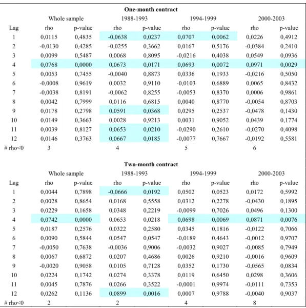
The first results, illustrated by Table 4, concern the autocorrelations between daily open-to-close returns for the two nearest contracts. We retained these two contracts because they are representative of six others, whose results are transferred in Appendix 3. Autocorrelations are estimated during each year sub-period. Table 4 also includes p-values associated with the autocorrelations.
Our main result is that autocorrelations are always positive and significant at lag 4 for all contracts. It is quite surprising to note that the behaviour of the 8 futures contracts does not differ in terms of autocorrelations. One would have expected that autocorrelations would change with liquidity and consequently with maturity. However, this is obviously not the case, even if the first month contract exhibits a number of significant autocorrelations that is a bit more important. It is also disappointing to observe a peak in autocorrelation at this lag, because there is no convincing explanation for it.
Another result is that negative autocorrelations tend to increase on the sample period, and they become dominant for certain maturities (2, 3, 6 and 7 months), at the end of the sample period. However the correlation coefficients are often not significant. Thus, the study of autocorrelations between open-to-close returns is not really satisfying. We extended it by examining these autocorrelations as a function of the time to expiration of the first month futures contract. Indeed, we
supposed that there could be some supplementary noise trading as the contract reaches maturity. However, this investigation did not lead us to new conclusions.
Table 4. Autocorrelations of close-to-open returns, for lags 1 to 12
One-month contract
Whole sample 1988-1993 1994-1999 2000-2003
Lag rho p-value rho p-value rho p-value rho p-value 1 0,0115 0,4835 -0,0638 0,0237 0,0707 0,0062 0,0226 0,4912 2 -0,0130 0,4285 -0,0255 0,3662 0,0167 0,5176 -0,0384 0,2410 3 0,0099 0,5487 0,0068 0,8095 -0,0216 0,4038 0,0549 0,0936 4 0,0768 0,0000 0,0673 0,0171 0,0693 0,0072 0,0971 0,0029 5 0,0053 0,7455 -0,0040 0,8873 0,0336 0,1933 -0,0216 0,5050 6 -0,0008 0,9619 0,0032 0,9110 -0,0103 0,6889 0,0065 0,8432 7 -0,0038 0,8191 -0,0062 0,8255 -0,0053 0,8370 0,0006 0,9861 8 0,0042 0,7999 0,0116 0,6815 0,0040 0,8770 -0,0054 0,8703 9 0,0178 0,2798 0,0591 0,0368 0,0295 0,2537 -0,0478 0,1430 10 0,0149 0,3663 0,0028 0,9213 0,0031 0,9052 0,0439 0,1774 11 0,0039 0,8127 0,0653 0,0210 -0,0290 0,2610 -0,0270 0,4098 12 0,0146 0,3763 0,0667 0,0185 -0,0077 0,7667 -0,0192 0,5581 # rho<0 3 4 5 6 Two-month contract Whole sample 1988-1993 1994-1999 2000-2003
Lag rho p-value rho p-value rho p-value rho p-value 1 0,0044 0,7898 -0,0666 0,0192 0,0502 0,0523 0,0172 0,5992 2 0,0028 0,8654 0,0168 0,5558 0,0312 0,2278 -0,0430 0,1895 3 0,0229 0,1658 0,0348 0,2219 -0,0099 0,7026 0,0496 0,1300 4 0,0742 0,0000 0,0653 0,0218 0,0698 0,0069 0,0871 0,0076 5 0,0187 0,2576 0,0322 0,2580 0,0345 0,1816 -0,0122 0,7066 6 0,0090 0,5844 0,0547 0,0547 -0,0189 0,4643 -0,0012 0,9707 7 -0,0050 0,7638 -0,0036 0,9006 -0,0032 0,9027 -0,0085 0,7949 8 0,0067 0,6872 0,0207 0,4686 0,0026 0,9210 -0,0016 0,9609 9 -0,0020 0,9058 0,0105 0,7128 0,0352 0,1730 -0,0565 0,0834 10 0,0224 0,1742 0,0274 0,3378 0,0119 0,6450 0,0298 0,3606 11 0,0045 0,7876 0,0266 0,3522 -0,0001 0,9974 -0,0111 0,7353 12 0,0262 0,1136 0,0899 0,0016 0,0007 0,9788 -0,0040 0,9037 # rho<0 2 2 4 8
● Autocorrelations of close-to-close returns
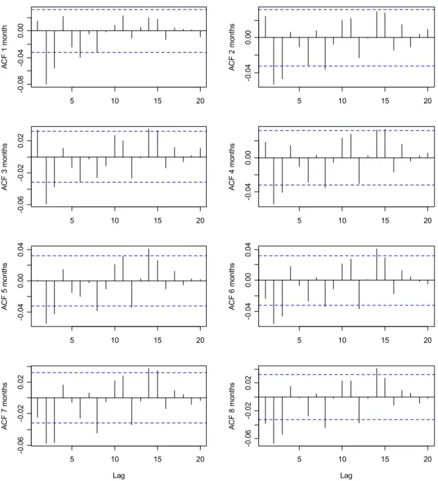
Turning now to the autocorrelations of close-to-close returns, the results are totally different. Figure 7 displays the results obtained, for the eight contracts, at lag 1 to 20, for the whole period. Autocorrelations are significant when the autocorrelation function pass the dotted line.
The first important observation is that now, there are often large and significant negative autocorrelations, for all contracts. Moreover, there is systematically a peak of autocorrelation at lag 2. Thus, including the electronic session in the trading period significantly modifies the autocorrelations
of the returns. One could infer of this result that there is noise trading during the night, which lasts almost two days. This supplementary noise could be due to the lack of volume during the night, which was mentioned when studying the overnight/trading ratios (Table 1). More impact is given to this assumption by the fact that autocorrelations become all the more significant that maturity rises. Indeed, this last observation shows that noise trading increases when the liquidity of the futures contract diminishes.
Figure 7. Autocorrelation function of close-to-close returns at lags 1 to 20, for the 8 nearest maturities 5 10 15 20 -0 .0 8 -0. 04 0. 00 A C F 1 m ont h 5 10 15 20 -0 .0 4 0.00 A C F 2 m ont hs 5 10 15 20 -0 .0 6 -0. 02 0. 02 AC F 3 m ont hs 5 10 15 20 -0 .0 4 0.0 0 AC F 4 m on th s 5 10 15 20 -0 .0 4 0.0 0 0.0 4 A C F 5 m ont hs 5 10 15 20 -0 .0 4 0.0 0 0.0 4 AC F 6 m on ths 5 10 15 20 -0 .0 6 -0. 02 0. 02 Lag A C F 7 m ont hs 5 10 15 20 -0 .0 6 -0 .02 0. 02 Lag A C F 8 m ont hs
As a conclusion on the study of autocorrelations, one could say that there seems to be noise trading in the crude oil market, and that part of this noise is generated by the electronic trading system. Another way to give evidence of the presence of noise trading is to compare the variances computed on daily returns (which reflect information and pricing errors) with variances for a long holding period (which reflect solely information). This constitutes the next step of the study.
3.2.2.2 Comparison of daily return variances with variances for a long holding period.
The comparison of daily variances with variances for a longer holding period relies on the assumption that the importance of pricing errors diminishes as the holding period increases. Indeed, if daily returns were totally independent, the variance for a long holding period would equal the cumulated daily variances within this period. On the other hand, if daily returns are temporarily affected by trading noise, the longer period variance will be smaller than the cumulated daily variances. Thus, the comparison will enable us to estimate the fraction of the daily variation that is caused by noise trading.
Table 5 reports average actual-to-implied variance ratios for holding periods of one, two, and three weeks, and one, three, and six months. These ratios are computed on a two-year period. The procedure used to obtain these estimates is the following. In order to compute, for example, the weekly actual-to-implied variance ratio for a given futures contract in a particular two-year subperiod9, we first calculate the average trading day return during the 104 weeks in that period10. Next, we cumulate the daily squared deviations around this average. Then, under the assumption that the daily returns are independent, we estimate the implied weekly variance by dividing this total by 104. Finally, we divide the actual weekly variance by the implied variance. The same procedure is used to estimate variance ratios for other holding periods.
9Motivation for the choice of a two-year period is twofold: first, this period is long enough to provide precise estimates for
the parameters; second, two years represent an efficient breakpoint in order to avoid non-stationarity problems.
10This is an example. Actually, we computed the number of daily returns on each sub-period, for each contract. Moreover,
we computed variances with rolling windows – of one, two and three weeks and of one, three and six months – in order to have a sufficient number of observations.
Table 5. Actual-to-implied variance ratios Actual-to-implied 1 week 1 month 2 months 3 months 4 months 5 months 6 months 7 months 8 months 1990-91 1,1296 1,0636 1,1041 1,0866 0,8540 0,8422 0,8644 0,8704 1992-93 0,7406 0,6872 0,7204 0,6877 0,7114 0,6482 0,6398 0,7065 1994-95 0,8794 0,8444 0,8371 0,8545 0,7869 0,8053 0,8195 0,6974 1996-97 0,8398 0,8859 0,8541 0,8051 0,7824 0,7443 0,8128 0,6924 1998-99 0,9953 0,9388 0,9482 0,9092 0,8962 0,9206 0,9113 0,6715 2000-01 1,0227 1,1169 1,1765 1,0705 0,9674 0,9142 1,1265 0,6919 2002-03 0,9938 0,9674 0,9723 0,9517 0,9129 0,8909 0,8920 0,9637 average 0,9430 0,9292 0,9446 0,9093 0,8445 0,8237 0,8666 0,7563 std dev 0,1305 0,1429 0,1581 0,1427 0,0889 0,0999 0,1454 0,1136 Actual-to-implied 2 weeks 1 month 2 months 3 months 4 months 5 months 6 months 7 months 8 months 1990-91 0,8907 0,8904 0,8957 0,9369 0,7164 0,7146 0,7108 0,6638 1992-93 0,7971 0,7493 0,7623 0,7468 0,7945 0,7272 0,7211 0,8031 1994-95 0,6984 0,6993 0,6600 0,6528 0,6158 0,6342 0,6346 0,5540 1996-97 0,7601 0,8662 0,8636 0,8134 0,8168 0,7160 0,8023 0,6335 1998-99 0,8885 0,8641 0,8725 0,8556 0,8479 0,8756 0,8487 0,6118 2000-01 0,7999 0,8599 0,8815 0,7902 0,6689 0,6985 0,6996 0,4843 2002-03 0,8696 0,8947 0,9186 0,9091 0,9034 0,8701 0,9126 0,9376 average 0,8149 0,8320 0,8363 0,8150 0,7662 0,7480 0,7614 0,6697 std dev 0,0722 0,0761 0,0922 0,0974 0,1028 0,0905 0,0968 0,1538 Actual-to-implied 3 weeks 1 month 2 months 3 months 4 months 5 months 6 months 7 months 8 months 1990-91 0,8580 0,8597 0,8774 0,9424 0,7127 0,7237 0,7288 0,6664 1992-93 0,7106 0,6759 0,6873 0,6751 0,7150 0,6558 0,6631 0,7565 1994-95 0,5986 0,6028 0,5815 0,5789 0,5404 0,5541 0,5281 0,4482 1996-97 0,6978 0,8330 0,8557 0,8130 0,7984 0,6496 0,7835 0,6180 1998-99 0,7974 0,8043 0,8117 0,8046 0,7929 0,8221 0,7652 0,5937 2000-01 0,7577 0,7897 0,8031 0,7377 0,6371 0,6481 0,7049 0,4731 2002-03 0,7173 0,7676 0,8143 0,8229 0,7928 0,7937 0,8362 0,8156 average 0,7339 0,7618 0,7758 0,7678 0,7128 0,6924 0,7157 0,6245 std dev 0,0821 0,0912 0,1047 0,1170 0,0963 0,0934 0,0999 0,1358
The results in Table 5 indicate that a significant fraction of the daily variance is caused by pricing errors. Indeed, most of the time, the actual-to-implied variance ratio is inferior to one, and it diminishes when the length of the holding period increases. This supports the assumption that pricing errors do not affect futures prices in the long run. For example, the average six-month actual-to-implied variance ratio for the nearby futures contract is 0.54 on the period. We can infer that 46% of the daily variance of this futures contract is eliminated in the long run. Thus, pricing errors have relatively little effect on six-month holding period returns and, as far as the six month holding period
is considered, this phenomenon is more important at the end of the period. This could be to the increase in the liquidity of the nearest contracts observed in section 2.
Table 5 (Continued) Actual-to-implied 1 month 1 month 2 months 3 months 4 months 5 months 6 months 7 months 8 months 1990-91 0,7620 0,7370 0,7580 0,7912 0,6308 0,6576 0,6462 0,5566 1992-93 0,5820 0,5790 0,5743 0,5732 0,6328 0,5909 0,5716 0,6069 1994-95 0,5539 0,6224 0,5842 0,5813 0,5553 0,5387 0,5253 0,4868 1996-97 0,5421 0,6728 0,6854 0,6573 0,6456 0,5431 0,6496 0,5493 1998-99 0,6918 0,7186 0,7285 0,7261 0,7121 0,7341 0,6885 0,5165 2000-01 0,6504 0,7191 0,7407 0,6664 0,6119 0,6348 0,6783 0,5019 2002-03 0,7485 0,7721 0,8109 0,8182 0,7644 0,7666 0,8108 0,7968 average 0,6304 0,6748 0,6785 0,6659 0,6314 0,6165 0,6266 0,5363 std dev 0,0866 0,0627 0,0806 0,0839 0,0508 0,0748 0,0643 0,0438 Actual-to-implied 3 months 1 month 2 months 3 months 4 months 5 months 6 months 7 months 8 months 1990-91 1,0888 1,0048 1,0554 1,0377 0,7876 0,7791 0,7557 0,6633 1992-93 0,5984 0,6279 0,6417 0,6792 0,7745 0,7604 0,7500 0,7377 1994-95 0,5525 0,6005 0,5682 0,5789 0,5753 0,5559 0,5312 0,4813 1996-97 0,4892 0,6382 0,7032 0,7047 0,7128 0,5871 0,7209 0,6073 1998-99 0,6818 0,7639 0,8406 0,8777 0,9336 1,0181 0,9693 0,7211 2000-01 0,3917 0,4538 0,5114 0,5123 0,4834 0,5256 0,5826 0,4166 2002-03 0,4884 0,4919 0,4949 0,4979 0,4690 0,4571 0,4815 0,4703 average 0,6337 0,6815 0,7201 0,7317 0,7112 0,7043 0,7183 0,6046 std dev 0,2436 0,1868 0,2000 0,1949 0,1611 0,1870 0,1541 0,1306 Actual-to-implied 6 months 1 month 2 months 3 months 4 months 5 months 6 months 7 months 8 months 1990-91 0,7373 0,7059 0,7328 0,7382 0,5543 0,5477 0,5335 0,4719 1992-93 0,5911 0,5855 0,5811 0,6171 0,6884 0,6642 0,6536 0,7229 1994-95 0,4000 0,4120 0,3701 0,4022 0,3899 0,3888 0,3826 0,3369 1996-97 0,4167 0,6188 0,7306 0,7670 0,7808 0,6303 0,8371 0,7260 1998-99 0,6438 0,7944 0,9195 0,9906 1,0851 1,1869 1,1585 0,9020 2000-01 0,4262 0,4851 0,5329 0,5313 0,5110 0,5525 0,6223 0,4542 2002-03 0,2244 0,2079 0,2047 0,2026 0,1906 0,1861 0,1985 0,2014 average 0,5359 0,6003 0,6445 0,6744 0,6682 0,6617 0,6979 0,6023 std dev 0,1414 0,1401 0,1911 0,2052 0,2458 0,2743 0,2704 0,2140
It must also be noted that sometimes, the values are superior to one. Except for the one-week holding period, this phenomenon always coincides with the 1990-1991 sub-period, namely the period of the first Gulf War. At that time, the rate of information arrival was so high that the actual variance was higher than the implied variance.
3.2.3. Is noise trading really important?
The last part of the study consists in determining if noise trading is really responsible of the high variance recorded during trading hours. In other words, it allows disentangling, among the possible explanations of this phenomenon, between the information arrival component and the noise trading component.
To obtain that result, two kinds of variance ratios are used. The first are the variance ratios of Table 3, which represent simple indicators of the relative importance of trading, overnight and week-end variances. These ratios are fare less important than they should be if hourly returns were constant across trading and non trading periods. Are these low variance ratios caused by a reduction in the arrival of information when the exchange are closed or / and by a reduction of pricing errors due to trading? An answer can be given to that question using both these variance ratio and the actual to implied variance ratios.
Using this comparison, we examine what would be the level of the variance ratios if there were as much noise during the open outcry session, during the night, and during the week-end. The method presented below concerns the ratios of the week-end variance over the trading day variance. The same is applied for the ratios overnight/trading.
Suppose each day’s return (Rt) is made up of two components: a rational information component (Xt) and a mispricing component (Zt):
Rt = Xt + Zt
Then, assume that the variances of the trading day pricing errors are as large as the variances of week-end errors. Then the trading and weekend returns (Rttand Rwt) can be written as:
Rtt = Xtt + Zt
Rwt = Xwt + Zt
Based on the average ratios in Table 3, the average variance of Rwt is 0.649 time the variance of Rtt for the nearby futures contract:
Var (Xwt + Zt) = 0.649 Var (Xtt + Zt)
The average six-month variances ratio for the first month contract, and for the whole period, is 0.536. Let us assume that this ratio applies to the weekend variance:
Var (Xwt ) = 0.536 Var (Xwt + Zt)
Lastly, if pricing errors have a negligible effect on six-month returns, the six-month variance ratios in Table 5 can be written as:
Var (Zt) = (1 – 0.536) Var (Xwt + Zt)
Under the assumption that the information and mispricing components are independent, these equations can be combined to eliminate the pricing error variances,
Var (Xwt ) = 0.4977 Var (Xtt)
Eliminating the effect of these errors diminishes the average weekend-to-trading ratio by more than 15%. It appears, as is shown in table 10 – which presents the entire results, maturity by maturity, both for the week-end/trading and for the overnight/trading – that the same observation can be reached, most of the time, for the two ratios, for each maturity, and for each two-years periods.
Table 6. Changes recorded in the variance ratios of table 3 (in percentages), if there were as much noise during the open outcry session, during the night, and during the week-end.
1 month 2 months 3 months 4 months 5 months 6 months 7 months 8 months
1990-91 31,45 49,84 6,61 30,82 155,17 123,98 164,36 103,36 1992-93 -12,50 -13,30 -12,91 -10,01 -7,89 -9,21 -9,91 -7,97 1994-95 -20,45 -21,08 -21,89 -19,93 -19,94 -20,94 -22,82 -25,27 1996-97 -10,76 -9,79 -6,92 -6,15 -5,73 -11,10 -4,06 -7,55 1998-99 -0,97 1,56 -1,08 -0,15 0,15 -6,28 -1,56 1,83 2000-01 -20,87 -17,22 -14,07 -14,17 -11,87 -10,31 -11,46 50,28 2002-03 -31,14 -29,66 -30,67 -35,43 -35,46 -35,27 -38,36 -34,12 Average -15,14 -11,34 -10,73 -9,29 -8,93 -8,25 -7,48 -8,31
1 month 2 months 3 months 4 months 5 months 6 months 7 months 8 months
1990-91 -0,39 24,89 -7,34 -6,77 192,56 67,30 56,65 -12,77 1992-93 -10,70 -12,22 -11,83 -9,64 -7,57 -8,84 -9,77 -7,82 1994-95 -13,53 -14,56 -15,65 -14,81 -14,41 -13,64 -18,41 -21,92 1996-97 -18,16 -10,34 -6,76 -5,15 -4,80 -10,31 -4,09 -7,86 1998-99 -9,40 -5,63 -2,09 -0,24 2,04 4,15 3,40 -2,38 2000-01 -20,92 -16,78 -14,74 -14,94 -16,53 -14,72 -10,81 -16,31 2002-03 -35,23 -36,93 -36,75 -36,35 -36,09 -39,05 -38,35 -34,32 Average -15,23 -12,69 -10,55 -9,43 -9,98 -9,94 -8,60 -12,36 Week-end/Trading Overnight/Trading
Table 6 shows that, as one could have suspected with the study of the autocorrelations, there is noise trading during the night, and during the week-end. Moreover, this noise is a bit higher during the
period of electronic trading. Lastly, one exception must be mentioned: the Gulf War period, during which, obviously, there was noise trading during the open outcry session.
Thus, it appears that the low variance ratios, in table 3, are caused mainly by a reduction in the arrival of information when the open outcry session is over. This doesn’t mean, however, that there is no noise trading at all during the open outcry session. Remember that the estimates in Table 5 suggest that a quite important fraction of the daily variance is caused by pricing errors.
SECTION 4. CONTRIBUTION TO THE PRICE DISCOVERY PROCESS
To further investigate the extent to which the open outcry session, the overnight electronic trading period and the week-end electronic trading session affect the price process, we computed the contribution of each of the three sub-periods to the cumulated price variation over a 6-month period. As 6-month returns should not be affected by pricing error, our methodology allows us to study how the different trading protocols contribute to the incorporation of information into prices. To do so, we use the Weighted Price Contribution (WPC) estimator developed by Cao, Ghysels and Hatheway (2000). We shall first develop our methodology before turning to the estimation results and their interpretation.
4.1. Methodology
Denoting
∆
P
t the price variation from day(
t
−
1
)
close to dayt
close,t t
i
P
P
∆
∆
,/
(1)where is the price change for sub-period
i
on dayt
, and measures the contribution of the change that occurred on sub-period to the total price change on dayt
. In our framework, i will refer to the open-outcry trading period, to the overnight electronic trading period and i to the week-end trading period. Definition (1) is not satisfactory due to heteroscedastic issues: to see this, notice that small total price changes will give rise to high (if not infinite) contributions thus upward tilting the contributions during low volatility periods. To fix this problem, Cao et al. proposed the following weighting scheme:t i
P
,∆
i
=1 3 = 2 = i tP
∆
∑
∑
= = ∆ ∆ × ∆ ∆ = T t t t i T t t t i P P P P WPC 1 , 1 (2)in which the contribution measure (1) is scaled down according to a factor which measures the contribution of price change in the total price change over
t
1KT (in absolute terms).A further refinement, with respect to (2), consists in taking into account the different time lengths for the several sub-periods of interests. This yields the relative time-weighted price contribution (RTWPC) indicator for each period :
i
∑
∑
= ′ ′ ==
T t t i i T t t i i i iWPC
WPC
RTWPC
1 , 1 , /Time
/
Time
/
which measures the hourly rate at which information gets incorporated into prices. 4.2. Results
The results for the estimation of the WPC and RTWPC over our sample period are reported in Table 6.
Table 6. Weighted Price Contribution (WPC) and Relative Time-Weighted Price Contribution (RTWPC) for the 3 trading sessions over the sample period.
1 month 72.69 20.95 6.37 11.18 5.04 0.51 2 months 71.39 22.09 6.49 9.58 6.48 0.68 3 months 71.64 21.84 6.50 10.38 6.15 0.65 4 months 72.68 20.86 6.46 10.53 10.52 1.16 5 months 71.29 21.70 6.98 9.96 9.17 1.01 6 months 68.55 23.49 7.93 8.61 5.65 0.73 7 months 66.90 24.86 8.22 7.71 5.04 0.69 8 months 63.28 28.04 8.68 6.37 4.52 0.71 WPC (%) RTWPC Maturity 3 / 1 RTWPC 2 / 1 RTWPC RTWPC2/3 1 WPC WPC2 WPC3
Results based on the WPC measure clearly indicate that most of the price discovery process occurs during the open-outcry trading session, which accounts for 70% on average of the total price change. 23% of the price change occur during the electronic night trading session whereas the week-end only accounts for about 7%. A striking feature in Table 6 is the apparent decrease in the
contribution of the open-outcry session for maturities longer than 5 months. We formally investigated this issue through an OLS regression of the form:
ε
β
α
+
+
=
L iMAT
WPC
(3)where is a dummy variable which takes value 1 for maturities strictly longer than 5 months and 0 otherwise.
L
MAT
Table 7. Weighted Price Contribution (WPC) and contract maturity
WPC1 = α + β MATL 0,719 -0,057 (96.92) (-4.70) WPC2 = α + β MATL 0,215 0,040 (35.95) (4.07) WPC3 = α + β MATL 0,066 0,017 (20.50) (3.28)
Estimates in Table 7 confirm a significant decrease in WPC for longer maturities and, meanwhile, a significant increase in WPC andWPC . The explanation we give for this finding is related to liquidity: the greater the number of trades, the more information gets incorporated into prices through the trading process, so that the overnight and the week-end trading session contribute to a lower degree to the price discovery process.
1
2 3
Results based on the RTWPC measure confirm that the open-outcry session play a crucial role as the rate at which information is incorporated into price is 9.29 times greater (on average) compared with the night electronic trading session, and 6.57 greater compared with the week-end trading session. However, we get a different conclusion regarding the importance of the night electronic session compared with the week-end session as the information gets incorporated 1.3 times faster in the latter compared with the former. Our explanation for this finding is that information is more likely to occur during the week-end (in connection with business activity in the Eastern countries) that during the night.
SECTION 5. CONCLUSION
Our study of the American crude oil futures market leads us to several results.
A first inspection of the evolution of the volatility of settlement futures prices shows that, during the period, there is also a rise in volatility, which affects more particularly the nearest futures prices. Two explanations can be invoked to explain this phenomenon: it could be the result of the deregulation in the energy markets, and/or it could be a consequence of trading practices.
The remaining of the study on volatility aims to check whether the presence of a futures market induces a supplementary volatility. We observe, first of all, that trading variances are higher than overnight variances, which in return are higher than week-end variances. This lead us to conclude that there are two possible explanations of this peak of volatility during exchange trading hours: i) whereas the crude oil market is a worldwide market, information arrives only during the exchange trading hours, ii) there is excess volatility (ie mispricing errors) caused by trading. In order to disentangle between these two components of volatility, we first tried to identify the presence of noise trading in the crude oil market. Second, we measured the impact of noise trading on the higher volatility recorded during trading hours.
In order to give evidence of the presence of noise trading, we first studied the autocorrelations of daily returns. We concluded that there is noise trading in the crude oil market, and that part of this noise is generated by the electronic trading system. Then, comparing daily variances with variances for a longer holding period, we confirmed that a significant part of the daily variance is eliminated in the long run, and consequently, that a significant fraction of the daily variance is caused by pricing errors. Lastly, the study of the impact of noise trading on the volatility shows that, even if there is such noise in the crude oil market, the phenomenon of higher volatility recorded during trading hours is mainly due to the arrival of information.
The study of the contribution of the different trading periods to the price discovery process confirms that result. More precisely, it shows that the open outcry session plays a crucial role in the incorporation of information into prices. The overnight and the week-end trading sessions contribute to a much lower degree to the price discovery process. The explanation for that phenomenon lies
probably in the liquidity of the market: the greater the number of trades, the more quickly is information incorporated into prices.
REFERENCES
Booth, G. G., & Ciner, C., 2001. Linkages among agricultural commodity futures prices: evidence from Tokyo, Applied Economics Letters, May, 8(5).
Chow, Y., 2001. Arbitrage, Risk Premium, and Cointegration Tests of the Efficiency of Futures Markets, Journal of Business Finance & Accounting, June, 28(5/6).
Ciner, C., 2001. On the long run relationship between gold and silver prices: A note, Global Finance Journal, 12(2), 299-303.
Ciner, C., 2002. Information content of volume: An investigation of Tokyo commodity futures markets, Pacific-Basin Finance Journal, April, 10(2), 201-215.
Cox C.C., 1976. Futures trading and market information, Journal of political economy, 84(6), 1215-1237.
Dawson, P.J. & White, B., 2002. Interdependencies between agricultural commodity futures prices on the Liffe, Journal of Futures Markets, March, 22(3), 269-280.
Ewing, B. T. & Harter, C. L., 2000. Co-movements of Alaska North Slope and UK Brent crude oil prices, Applied Economics Letters, August, 7(8), 553-558.
Fleming, J., & Ostdiek, B., 1999. The impact of energy derivatives on the crude oil market, Energy Economics, April, 21(2), 135-168.
Fortenbery, T. R., & Zapata, H.O., 1997. Valuation of price linkages between futures and cash markets for cheddar cheese, Journal of Futures Markets, May, 17(3), 279-301.
Foster, A., 1995. Volume-volatility relationships for crude oil futures markets, Journal of Futures Markets, Dec., 15(8), 929-952.
French, K.R., & Roll R., 1986. Stock return variances, the arrival of information and the reaction of traders, Journal of Financial Economics, 17, 5-26.
Girma, P. B., & Mougoue, M., 2002. An empirical examination of the relation between futures spreads, volatility, volume and open interest, Journal of Futures Markets, Nov, 22(11), 1083-2003. Hammoudeh, S., Li, H., & Bang J. 2003. Causality and volatility spillovers among petroleum prices of WTI, gasoline and heating oil in different locations, North American Journal of Economics & Finance, Mar., 14(1), p89.
Hassapis, C., & Kalyvitis, S., 1999. Cointegration and joint efficiency of international commodity markets, Quarterly Review of Economics & Finance, Summer, 39(2), 213-232.
Holt, M.T., 2002. Market efficiency in agricultural futures markets, Applied Economics, Aug., 34(12), 1519-1533.
Horsnell, P., & Mabro, R. 1993. Oil Markets and Prices. Oxford University Press.
Jones C.M., Kaul G., Lipson M.L., 1994. Information, trading and volatility. Journal of financial economics, 36, 127-154.
Jumah, A., & Karbuz, S., 1999. Interest rate differentials, market integration, and the efficiency of commodity futures markets, Applied Financial Economics, Feb., 9(1), p101-109.
Kellard, N., Newbold, P., 1999. The relative efficiency of commodity futures markets, Journal of Futures Markets, Jun., 19(4), 413-433.
King, J., 2001. Testing the Efficient Markets Hypothesis with Futures Markets Data: Forecast Errors, Model Predictions and Live Cattle, Australian Economic Papers, Dec., 40(4), 581-585.
Kleit, A. N., 2001. Are Regional Oil Markets Growing Closer Together? An Arbitrage Cost Approach, Energy Journal, 22(2), 1-15.
Kodres L., & Schachter B., 1996. CBOT futures options: the impact of options listing on the underlying market 1924-1926, CBOT symposium proceeding, Fall 1996 – Part I.
Leistikow, D., 1990. The Relative Responsiveness To Information And Variability Of Storable Commodity Spot And Futures Prices, Journal of Futures Markets, 10(4), 377-396.
Low, A. H.W., & Muthuswamy, J., 1999. Arbitrage, cointegration, and the joint dynamics of prices across discrete commodity futures, Journal of Futures Markets, Oct., 19(7), 799-816.
Mayhew S., 2000, The impact of derivatives on cash markets: what have we learned? Working Paper, University of Georgia, Athens.
Milonas, N. T., & Henker, T., 2001. Price spread and convenience yield behaviour in the international oil market, Applied Financial Economics, Feb., 11(1), 23-37.
Moosa, I. A., & Silvapulle, P., 2000. The price-volume relationship in the crude oil futures market, International Review of Economics & Finance, 9(1), 11-31.
Pindyck R., & Rotenberg J., 1990. The excess co-movement of commodity prices, Economic Journal, 100, 1173-89.
Samuelson P.A., 1965. Proof that properly anticipated prices fluctuate randomly. Industrial Management Review, 6, 41-49, Spring.
Sanjuán, A. I., & Gil, J. M., 2001. Price transmission analysis: a flexible methodological approach applied to European pork and lamb markets, Applied Economics, 33(1), 123-132.
Appendix 1. Variance ratios, Week-end/Trading and Overnight/Trading
1. Week-end/Trading
1 month 2 months 3 months 4 months 5 months 6 months 7 months 8 months 1989 0,29 0,46 0,42 0,43 0,44 0,42 0,41 0,46 1990 1,52 1,53 1,70 2,23 2,13 1,93 2,14 1,52 1991 1,46 1,62 0,60 0,74 1,09 1,15 1,03 1,25 1992 0,38 0,70 0,37 0,34 0,30 0,32 0,36 0,41 1993 0,53 0,42 0,55 0,35 0,39 0,46 0,48 0,55 1994 0,51 0,54 0,58 0,60 0,53 0,58 0,64 0,57 1995 0,40 0,49 0,33 0,27 0,31 0,33 0,42 0,47 1996 0,16 0,27 0,33 0,41 0,43 0,39 0,35 0,36 1997 0,25 0,41 0,40 0,39 0,36 0,54 0,40 0,48 1998 1,69 1,80 1,44 1,37 1,57 2,05 1,84 1,73 1999 0,27 0,32 0,27 0,22 0,40 0,58 0,37 0,56 2000 0,51 0,54 0,59 0,60 0,65 0,83 0,79 0,71 2001 0,78 0,82 0,86 0,85 0,99 0,82 0,49 1,77 2002 0,44 0,48 0,48 0,53 0,51 0,46 0,58 1,17 2003 0,54 0,39 0,42 0,58 0,56 0,58 0,80 0,47 Average 0,65 0,72 0,62 0,66 0,71 0,76 0,74 0,83 Std Err 0,49 0,50 0,41 0,52 0,53 0,54 0,55 0,51
2. Overnight/Trading
1 month 2 months 3 months 4 months 5 months 6 months 7 months 8 months 1989 0,87 0,49 0,32 0,27 0,27 0,28 0,26 0,34 1990 0,57 0,76 0,80 0,72 0,70 0,65 0,73 0,60 1991 1,41 1,98 0,51 0,67 2,64 2,14 1,95 1,08 1992 0,35 0,53 0,46 0,42 0,42 0,46 0,55 0,58 1993 0,34 0,31 0,31 0,23 0,23 0,26 0,27 0,32 1994 0,23 0,26 0,27 0,18 0,22 0,21 0,31 0,37 1995 0,28 0,32 0,30 0,40 0,32 0,30 0,42 0,45 1996 0,47 0,37 0,33 0,30 0,29 1,09 0,37 0,51 1997 0,32 0,37 0,36 0,28 0,28 0,33 0,39 0,44 1998 0,20 0,32 0,31 0,35 0,30 0,45 0,50 0,40 1999 0,51 0,59 0,65 0,62 0,67 0,69 0,74 0,90 2000 0,68 0,42 0,39 0,40 0,53 0,41 0,52 0,62 2001 0,59 0,50 0,52 0,53 0,56 0,72 0,88 0,94 2002 0,61 0,57 0,58 0,58 0,45 0,62 0,57 0,70 2003 0,64 0,70 0,64 0,60 0,65 0,65 0,83 0,94 Average 0,54 0,57 0,45 0,44 0,57 0,62 0,62 0,61 Std Err 0,31 0,42 0,16 0,17 0,60 0,48 0,42 0,25