Modeling of Sales Forecasting in Retail Using Soft Computing Techniques

(1)

Modeling of Sales Forecasting in Retail Using Soft

Computing Techniques

Lu´ıs Francisco Oliveira Martelo Lobo da Costa

Dissertaç ão para obtenç ão do Grau de Mestre em

Engenharia Mec ˆanica

J ´

uri

Presidente:

Prof. Jos ´e Rog ´erio Caldas Pinto

Orientador:

Prof. Jo ˜ao Miguel da Costa Sousa

Co-Orientador:

Dr. Susana Margarida da Silva Vieira

Vogais:

Eng. Hugo Miguel Lampreia Alexandre

Prof. Lu´ıs Manuel Fernandes Mendonc¸a

(2)

(3)

And the high destiny of the individual is to serve rather than to rule, or to impose himself in any other way.

Albert Einstein

The one thing that matters is the effort.

(4)

Este trabalho reflecte as ideias dos seus autores que, eventualmente, poderão não coincidir com as do Instituto Superior Técnico.

(5)

Abstract

The objective of this work is to address the problem of aggregate daily sales forecasting in retail. In-telligent modeling techniques were applied to this problem. Fuzzy classification and NARX models, feedforward classification and NARX neural networks and adaptive neuro-fuzzy systems were tested over three different forecasting periods in order to test the applicability of each model.

A methodology on how to select the forecasting periods is presented. The different forecasting horizons consist of a stationary period, where there are no major variations from a regular weekly pattern; a stationary period with disturbances, where there are some events that have an impact on the weekly pattern; and a non-stationary period, which is constituted by several different events that have major impacts on the sales behavior.

It is also presented a methodology on how to construct the models’ features. These features account the effects that major variables have on sales forecasting. These are the weekly and monthly seasonality, the macroeconomic environment translated into the purchasing power, the major promotions and holidays.

Further, each model’s parameters are developed. The models that presented accurate training per-formances are finally tested over the forecasting periods, allowing the obtention of accurate forecasts for the three periods, in particular considering stationary periods and well defined events.

(6)

(7)

Resumo

O objectivo deste trabalho aborda o problema da previsão de vendas agregadas no retalho. Na sua abordagem, foram utilizadas técnicas de modela¸cão inteligente. Classificadores fuzzy, modelos NARX fuzzy, redes neuronais de classifica¸cão e redes NARX, assim como sistemas neuro-fuzzy foram testados para três per´ıodos de predi¸cão diferentes, de forma a testar a aplicabilidade destes modelos.

A metodologia de seleçcão dos per´ıodos de predi¸cão é apresentada. Os diferentes horizontes temporais de predi¸cão consistem num per´ıodo estacionário, onde as vendas apresentam uma tendência semanal; um per´ıodo estacionário com perturba¸cões, onde alguns efeitos perturbam o padrão semanal usual; e um per´ıodo não-estacionário, constitu´ıdo maioritariamente por eventos que têm um impacto significativo no comportamento da curva de vendas.

´

E também apresentada a metodologia usada na constru¸cão dos atributos constituintes dos modelos. Estes atributos pretendem considerar os efeitos das principais variáveis de influência nas vendas. Nestes eventos englobam-se a sazonalidade semanal, sazonalidade mensal, a tradu¸cão do efeito macro-económico no poder de compra, as principais promo¸cões, e feriados ou principais dias festivos.

Após as anteriores defini¸cões, apresenta-se o desenvolvimento de cada modelo e dos parâmetros con-stituintes. Os modelos que melhor desempenho apresentaram no treino são usados para teste (ou seja, previsão), para cada um dos per´ıodos anteriormente definidos. Para cada per´ıodo, obtiveram-se resultados exactos, em particular para per´ıodos estacionários e eventos bem definidos.

(8)

(9)

Acknowledgements

I would like to acknowledge my supervisors Professor Jo˜ao Sousa and Doctor Susana Vieira for their guidance through this work. Their technical knowledge, good sense and optimism were very important to drive this work to a good end.

I would like to thank SONAE SR for the opportunity of developing this interesting project. It was a period of intense learning, and the experience was a rich complement to my education. I was able to develop skills that for sure will be useful in the future.

I would also like to thank Eng. Hugo Alexandre and his team, for receiving me, providing me all the information needed, and giving me great insights and ideas on how to develop this work. A special thanks to Jo˜ao Semeano, who shared this experience in the enterprise, and who was always available to discuss my doubts and to contribute with new ideas.

A special acknowledgement to my family, for being always present with words of support and encour-agement. To my parents, who always helped me to keep track and focused on the essential, and to my brother, a great company and with whom I spend incredible moments.

Finally, I would like to thank all my colleagues and friends that were present in these last years. Thankfully, you are so many that is impossible to thank each one of you for your amazing support here. You know who you are.

(10)

(11)

List of Figures

2.1 Model of a neuron . . . 20

2.2 Feedforward classification neural network . . . 22

2.3 NARX neural network . . . 23

2.4 Model of a neuron . . . 24

3.1 Weekly sales from weekaaof year A to the weekeeof year C per year . . . 28

3.2 Real sales against sales without seasonality and major promotions effects . . . 29

3.3 Yearly sales and yearly sales without seasonality and major promotions effect . . . 29

3.4 Daily sales in weeksaatobbfor all years together . . . 30

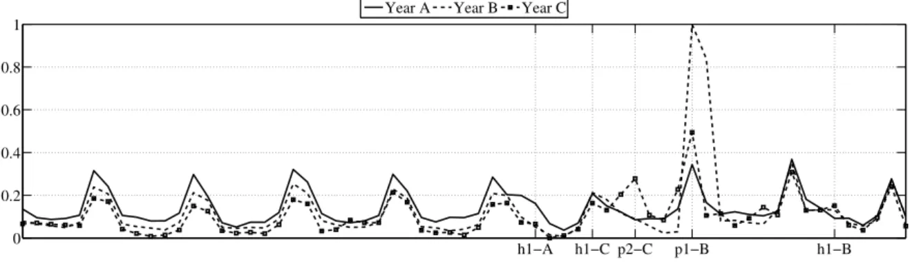
3.5 Daily sales in weeksaatoccfor all years together . . . 31

3.6 Daily sales in weeks 3 to 22 for all years together . . . 31

3.7 Weekly seasonality . . . 33

3.8 Monthly seasonality with weekly data . . . 34

3.9 Monthly seasonality . . . 34

3.10 Vector of daily sales for weeksaatobbfrom yearA toC. . . 35

3.11 Promotions in the data . . . 36

3.12 Promotions input . . . 38

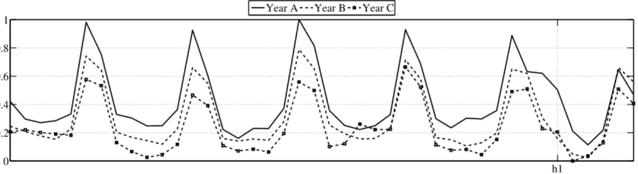
3.13 Type 1 holiday (h1) from yearAto C . . . 39

3.14 h2holiday and week before for each year . . . 40

3.15 Week of the type 3 holiday (h3) . . . 41

3.16 Holidays input . . . 42

3.17 All inputs . . . 43

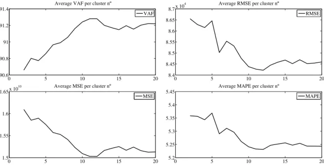
4.1 Performance per number of clusters for the classification fuzzy model - stationary period . 47 4.2 Performance per number of clusters for the NARX fuzzy model - stationary period . . . . 49

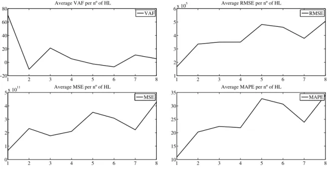
4.3 Performance per number of HL for the feedforward neural network - stationary period . . 50

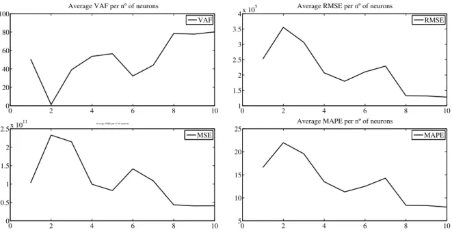
4.4 Performance per number of neurons in 1 HL for the feedforward neural network - stationary period . . . 51

4.5 Performance per number of HL for the NARX network - stationary period . . . 52

4.6 Performance per number of neurons in 1 HL for the NARX neural network - stationary period . . . 53

(16)

4.7 Performance per number of delays in a 7 single neuron HL NARX network - stationary

period . . . 54

4.8 Performance per number of membership functions for the ANFIS model - stationary period 55 5.1 Sales forecasting with the fuzzy classification model - Stationary period . . . 66

5.2 Comparison of all the results - Stationary period . . . 67

5.3 Sales forecasting with the fuzzy classification model - stationary period with disturbances 69 5.4 Comparison of all the results - stationary period with disturbances . . . 71

5.5 Sales forecasting with the fuzzy classification and NARX model - Non-stationary period . 72 5.6 Sales forecasting with the fuzzy classification model - Non-stationary period . . . 73

A.1 Yearly sales and yearly sales without seasonality and major promotions effect - zoom in weeks aato bb. . . 91

A.2 Performance per number of clusters for the classification fuzzy model . . . 92

A.3 Performance per number of clusters for the narx fuzzy model . . . 93

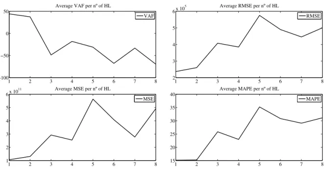
A.4 Performance per number of HL for the feedforward NN . . . 94

A.5 Performance per number of neurons per HL for the feedforward NN . . . 94

A.6 Performance per number of HL for the NARX NNl . . . 95

A.7 Performance per number of neurons in each HL for the NARX NNl . . . 96

A.8 Performance per number of delays in the NARX NNl . . . 96

A.9 Performance per number of clusters for the classification fuzzy model . . . 97

A.10 Performance per number of clusters in the fuzzy NARX . . . 98

A.11 Performance per number of HL in the feedforward NN . . . 98

A.12 Performance per number of neurons in the feedforward NN . . . 99

A.13 Performance per number of HL in the feedforward NN . . . 100

A.14 Performance per number of neurons in each HL for the NARX NN . . . 100

(17)

List of Tables

3.1 Weekly seasonality . . . 33 3.2 Monthly seasonality . . . 34 3.3 Purchasing power . . . 35 3.4 Promotion input . . . 38 3.5 Type 1 effect . . . 39 3.6 Type 2 effect . . . 40

3.7 Type 3 holidays input . . . 42

3.8 Prediction periods . . . 43

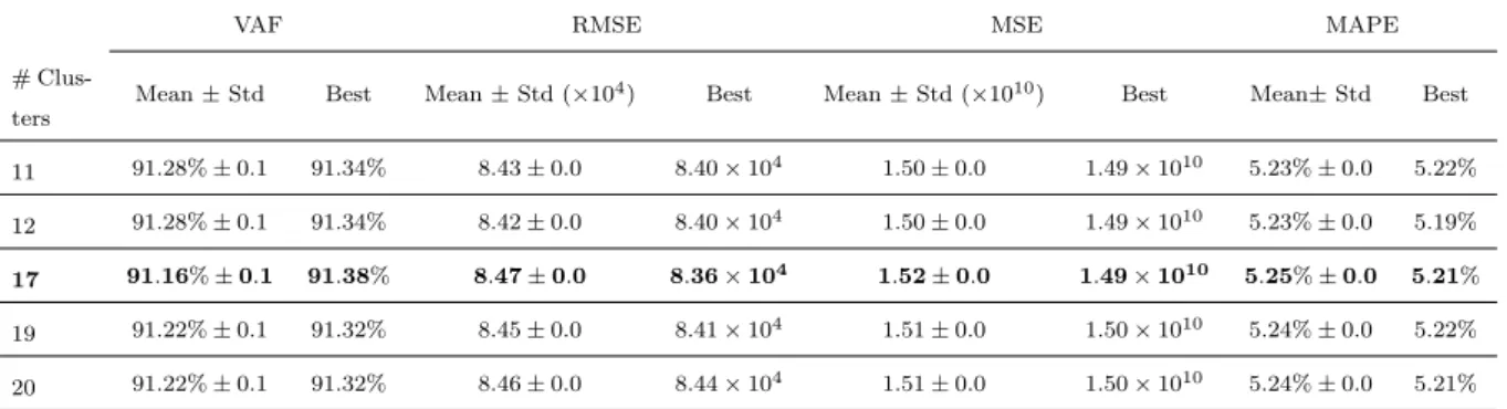
4.1 Performance per number of clusters for the classification model - stationary period . . . . 48

4.2 Performance per number of clusters for the NARX fuzzy model - stationary period . . . . 49

4.3 Performance per number of HL for the feedforward network - stationary period . . . 50

4.4 Performance per number of neurons in 1 HL for the feedforward network - stationary period 51 4.5 Performance per number of HL for the NARX network - stationary period . . . 52

4.6 Performance per number of neurons in each HL for the NARX network - stationary period 53 4.7 Performance per number of delays in a 7 single neuron HL NARX network - stationary period . . . 54

4.8 Performance per number of membership functions for the ANFIS model - stationary period 55 4.9 Performance per number of clusters for the classification model - stationary period with disturbances . . . 56

4.10 Performance per number of clusters for the NARX fuzzy model - stationary period with disturbances . . . 56

4.11 Performance per number of HL for the feedforward network - stationary period with dis-turbances . . . 57

4.12 Performance per number of neurons in each HL for the feedforward network - stationary period with disturbances . . . 57

4.13 Performance per number of HL for the NARX network - stationary period with disturbances 58 4.14 Performance per number of neurons in each HL for the NARX network - stationary period with disturbances . . . 58

4.15 Performance per number of delays for the NARX network - stationary period with distur-bances . . . 58

(18)

4.16 Performance per number of membership functions for the ANFIS model - stationary period

with disturbances . . . 59

4.17 Performance per number of clusters for the classification model - non-stationary period . . 59

4.18 Performance per number of clusters for the NARX model - non-stationary period . . . 60

4.19 Performance per number of HL for the feedforward network - non-stationary period . . . 60

4.20 Performance per number of neurons in each for the feedforward network - non-stationary period . . . 60

4.21 Performance per number of HL for the NARX network - non-stationary period . . . 61

4.22 Performance per number of neurons in each HL for the NARX network - non-stationary period . . . 61

4.23 Performance per number of delays for the NARX network - non-stationary period . . . . 61

4.24 Performance per number of membership functions for the ANFIS model - stationary period with disturbances . . . 62

4.25 Performance of each model in the stationary period . . . 62

4.26 Performance of each model in the stationary period with disturbances . . . 63

4.27 Performance of each model in the non-stationary period . . . 63

5.1 Comparison of the best models in testing - stationary period . . . 66

5.2 Application of the fuzzy classification model to the different business units - stationary period . . . 68

5.3 Comparison of the best models in testing - stationary period with disturbances . . . 69

5.4 Application of the fuzzy classification model to the different business units - stationary period with disturbances . . . 71

5.5 Comparison of the best models in testing - non-stationary period . . . 72

5.6 New classification best model performance - non-stationary period . . . 73

5.7 Application of the fuzzy classification model to the different business units - non-stationary period . . . 75

A.1 Performance per number of clusters for the classification model - stationary period with disturbances . . . 92

A.2 Performance per number of clusters for the NARX fuzzy model - stationary period with disturbances . . . 93

A.3 Performance per number of HL for the feedforward network - stationary period with dis-turbances . . . 94

A.4 Performance per number of neurons in each HL for the feedforward network - stationary period with disturbances . . . 95

A.5 Performance per number of HL for the NARX network - stationary period with disturbances 95 A.6 Performance per number of neurons in each HL for the NARX network - stationary period with disturbances . . . 96

(19)

A.7 Performance per number of delays for the NARX network - stationary period with distur-bances . . . 97 A.8 Performance per number of clusters for the classification model - non-stationary period . . 97 A.9 Performance per number of clusters for the NARX model - non-stationary period . . . 98 A.10 Performance per number of HL for the feedforward network - non-stationary period . . . 99 A.11 Performance per number of neurons in each for the feedforward network - non-stationary

period . . . 99 A.12 Performance per number of HL for the NARX network - non-stationary period . . . 100 A.13 Performance per number of neurons in each HL for the NARX network - non-stationary

period . . . 101 A.14 Performance per number of delays for the NARX network - non-stationary period . . . . 101

(20)

(21)

Notation

Symbols

Ai – Fuzzy set of the antecedent

Bi – Fuzzy set of the consequent

Ri – Fuzzy rule K – Number of rules x – Data sample X – Database ˆ y – Model output y – System output µA(x),µB(y) – Menmbership functions µR(x,y) – Fuzzy relation

fi – Mapping function of theith rule

βi – Degree of fulfullment of rulei

vi – Cluster center

J – Objective function

U – Fuzzy partition matrix V – Matrix of cluster prototypes D2

ijA – Inner-product distance norm

A – Non-inducing matrix that determines cluster shape

λ – Lagrange multipliers

πi – Parameter vector for the ithrule θ – Matrix of model parameters

(22)

Ψ – Matrix of vector inputs Φ – Vector containing the regressor Υ – Vector containing the regressand

Γ – Matrix containing the membership degree

xkj – Neuron input

wkj – Weight factor

z – Weighted sum of the neuron inputs bj – Constant input, bias or threshold

[xj,1]T – Expanded input vector [wT

j, bj] – Weights vector

ϕj(z) – Neuron output

ϕj – Activation function

f(x) – Output of the neural network

t – Time

dx – Delay on the inputs

dy – Delay on the outputs

wi – Firing strength

pi,qi andri – ANFIS node parameters

O – ANFIS node output

F – Function of the fuzzy inference system

H – Identity function s – Sales ws – Weekly seasonality ms – Monthly seasonality pw – Purchasing power p – Promotions h – Holidays

(23)

Acronyms

ANFIS – Adaptive neuro-fuzzy inference system ARIMA – Auto-regressive moving average

BET – Bucharest Stock Exchange Trading Index COG – Centre of gravity

FCM – Fuzzy C-means JIT – Just in time HL – Hidden layer

LSE – Least-squares estimator

MAPE – Mean absolute percentage error MAR – Missing at random

MCAR – Missing completely at random MISO – Multi-input single-output MLP – Multi-layer perceptron MOM – Mean of maxima MSE – Mean squared error

N – Neuron

NARX – Non-linear auto-regressive with exogenous input NN – Artificial neural networks

P – Parallel mode PCB – Printed circuit board POS – Point of sales

RMSE – Root mean squared error SP – Series-parallel mode TDNN – Time delay neural network TS – Takagi-Sugeno

VAF – Variance accounted for VBR – Variable bit rate

(24)

(25)

Chapter 1

Introduction

Due to the strong and growing competition existing nowadays, the majority of retailers are in a continuous effort for increasing profits and reducing costs [19]. In addition, the variations in consumers demand, which are caused by many factors like price, promotion, changing consumers’ preference, seasonality, or weather changes, contribute to a fluctuating market behavior [3].

In that sense, an accurate sales forecasting system is an efficient way to achieve higher profits and lower costs, by improving customers satisfaction, reducing product destruction, increasing sales revenue and desiging production plans efficiently [19].

Sales forecasting is the starting point for planning various phases of a firms operations [13], and a crucial task in supply chain management under dynamic market demand which, ultimately, affects retailers and other channel members in various ways [99]. Industry forecasts are especially useful to big retailers who may have a greater market share [3].

Due to ever-increasing global competition and an environment characterized by very short product life cycles and high market volatility [98], this subject plays an even more prominent role in supply chain management when the profitability and the long-term viability of a firm relies on effective and efficient sales forecasts [96]. Theoretically speaking, the way to improve the quality of forecasts is still an outstanding subject of attention [39]. For data containing trend and seasonal patterns, failure to account for these patterns may result in poor forecasts. Over the last few decades several methods such as Winters exponential smoothing, Box-Jenkins, autoregressive integrated moving average (ARIMA) model and multiple regression have been proposed and widely used to account for these patterns. More recently, artificial neural networks (NNs) have emerged as a technology with a great promise for identifying and modeling data patterns that are not easily described by traditional statistical methods in diverse areas as cognitive science, computer science, electrical engineering and finance [3].

Forecasting has earned global acceptance as a decisive part of business planning and decision-making in a diversity of areas such as sales planning, marketing research, pricing, production planning and scheduling [59],[75].

This chapter begins with the definition of sales forecasting, and its main variables. Afterwards is introduced the role that systems engineering and, more specifically, soft computing modeling techniques

(26)

have been having in sales forecasting. Finally, the main contributions of this work and its outline are presented.

1.1 Sales forecasting

Sales forecasting refers to the prediction of future sales based on past historical data. Owing to compe-tition and globalization, sales forecasting plays an even more important role as part of the commercial enterprise [98]. Accurate sales forecasting is crucial for profitable retail operations because without a good forecast, either too-much or too-little stocks would result, directly affecting the revenue and competitive position [1]. In that sense, forecasting models contribute to accurate sales estimates for a retailer, may allow its supply chain to effectively control the inventory to achieve just-in-time (JIT); scheduling and arranging the facility utilization, which decreases costs to the supplier, and, therefore, to the retailer [57]. The processes of science and decision making share an important characteristic: success in each depends upon the researcher or decision maker having some ability to anticipate the consequences of their actions [72]. Without sales forecasts, operations can only respond retroactively, leading to poor production planning, lost orders, inadequate customer service, and poorly utilized resources [35],[96].

Recent research has shown that effective sales forecasting enables improvements in supply chain per-formance [9],[96],[102]. Better forecasts of aggregate retail sales can improve the forecasts of individual retailers because changes in their sales levels are often systematic. For example, around Christmas time, sales of most retailers increase [3].

The growing importance of the forecasting function within companies is reflected in an increased level of commitment in terms of money, hiring of operational researchers and statisticians, and purchasing computer software [95].

In [75],[95], some factors which contributed to the importance of forecasting within organizations are pointed:

• “The increasing complexity of organizations (e.g. number of submarkets served and products of-fered) and their environments (e.g. changes in technology and demand structures) has made it more difficult for decision makers to take all the factors relating to the future development of the organization into account;”

• “Organizations have moved towards more systematic decision making that involves explicit jus-tifications for individual actions, and formalized forecasting is one way in which actions can be supported;”

• “The further development of forecasting methods and their practical application has allowed not only forecasting experts but also managers (decision makers) to understand and use these tech-niques, becoming useful tools within the hole organization.”

In process industries ranging from oil and gas industry [58], to the high-risk agrochemical and phar-maceutical industries [59],[64], customer demand has been clearly identified by recent studies as the top

(27)

business management driver. Given the importance of customer demand, it is easy to realize the potential surplus of an effective tool for customer demand forecasting in process industries [59].

Since managers in retails are waiting for a suitable tool to support their making the purchasing decisions, they usually rely on their own experience or consult the point of sales system (POS system) to predict the future sales and place purchasing orders. Few decision-makers adopt statistical methods, such as the moving average method or exponential smoothing, to deal with the daily problems commonly. In fact, most conventional sales forecasting methods use either factors or time-series data to determine the sales prediction. The relationship between the past time-series data and the sales prediction is always too complex to acquire an advantageous ordering suggestion by using the unsuited statistical approaches. Practically, the POS system actually provides some forecasting suggestions for the managers to place orders. However, most decision-makers still prefer to place the same quantity as usual or depend on their own intuition instead of model-based approaches. [19]

In the present, the variations in consumers demand are caused by many factors like price, promotion, changing consumer preference, seasonality, or weather changes [3]. Regarding conventional sales forecast-ing methods, most of them used either factors or time series data to determine the forecast. However, the relationship between the factors or the past time series data independent variables and the sales data dependent variable is always quite complicated [57]. Due to nature of the relationships among indepen-dent and depenindepen-dent variables, various computational intelligence methods have emerged over the last two decades as alternatives for building effective predictors. Some of these models are based on neural networks [101], fuzzy models, and hybrid approaches [68], adopting iterative adjustments of a unique model during a sequence of offline parameter updates, and considering all of the data available for the task at each iteration [62].

1.2 Intelligent computing techniques for sales forecasting

From an historical perspective, exponential smoothing methods and decomposition methods were the first forecasting approaches to be developed back in the mid-1950s. During the 1960s, as computer power became more available and cheaper, more sophisticated forecasting methods appeared [59].

Box–Jenckins [14] methodology gave rise to the ARIMA models [27], [37],[59], [83]. Later on, during the 1970s and 1980s, even more sophisticated forecasting approaches were developed including economet-ric methods and Bayesian methods [75].

Time series forecasting models have been widely applied in sales forecasting, such as exponential smoothing models [36],[51], ARIMA models [37], expert systems [61], fuzzy systems [16], [21], and NN models [23],[81],[96] [100].

Soft, or intelligent, computing algorithms, which combined fuzzy theory with neural network has found a variety of applications in various fields, ranging from industrial environment control system, process parameters, semi-conductor machine capacity forecasting, business environment forecasting, financial analysis, stock index fluctuation forecasting, consumer loan, medical diagnosis and electricity demand forecasting [22].

(28)

One of the major limitations of the traditional methods compared to soft computing is that they are essentially linear methods. In order to use them, users must specify the model form without the necessary genuine knowledge about the complex relationship in the data [23].

Forecasting with fuzzy systems is, generally, accomplished with a combination of other soft computing techniques such as neural networks or genetic algorithms; or a hybrid structure such as ANFIS. Kuo, [54], [55], [56], proposed a fuzzy neural networks with different approaches to learn fuzzy if-then rules for promotion, which were integrated in a neural network for forecasting using time series data. The model performed more accurately than statistical methods and single adaptive neural networks. In [17] a evolving fuzzy neural network was developed for PCB sales forecasting and states that the model can be applied practically as a sales forecasting tool in the PCB industry. ANFIS is used in [5] for estimation of Natural Gas demand. The model provides a better performance than adaptive neural networks and time series performance. ANFIS was used to forecast tourist arrivals in Taiwan in [20], and outperformed a fuzzy time series model, grey forecasting model and Markov residual model. [41] uses an approach based on genetic fuzzy systems and artificial neural networks for constructing a stock price forecasting expert system which outperformed previous methods. ANFIS was also used by [89] to forecast demand for thin-film transistor liquid display manufacturer and the model performed better than other four.

One nonlinear model that receives extensive attention in forecasting is the NN model [101]. Inspired by the architecture of the human brain as well as the way it processes information, NNs are able to learn from the data and experience, identify the pattern or trend, and make generalization to the future [23].

The idea of using NNs for forecasting is not new. The first application dates back to 1964. Hu, [44], in his thesis, uses the Widrows adaptive linear network to weather forecasting. Werbos, [93], [94], first formulates the backpropagation and finds that NNs trained with backpropagation outperform the traditional statistical methods such as regression and Box-Jenkins approaches [101].

Research efforts on NNs for forecasting are considerable. The literature is vast and growing. Marquez et al., [65], and Hill et al.,[43], review the literature comparing NNs with statistical models in time series forecasting and regression-based forecasting. However, their review focuses on the relative performance of NNs and includes only a few papers[101].

In [4], the use of back-propagation (BP) NN model was presented to analyze the behavior of sales in a medium size enterprise and reported that the BP model generated better forecasts than ARIMA models with interventions did. A NN-based forecasting system to predict the weekly product demand in a German supermarket company was also developed [85]. A comparison between traditional methods with artificial neural networks forecasting aggregate sales was made and concluded that the NN model was able to effectively capture the dynamic nonlinear trend and seasonal patterns, as well as the interactions between them [3]. In [23] another comparison of the performance of NN models and various linear models for forecasting aggregate retail sales and reported that the overall best model is the NN model built on deseasonalized time series data. A proposed evolving NN forecasting model by integrating genetic algorithms and BP NN was concluded to generate more accurate forecasts than traditional statistical models and BP networks in [18].

(29)

Mackey-Glass time series by Lapedes and Farber, where the feedforward neural networks that can accu-rately mimic and predict such non linear systems was designed. Also related with chaotic time-series, [30] propose a hierarchically trained NN model in which a dramatic improvement in accuracy is achieved for prediction of two chaotic systems.

A series often used as a yardstick to evaluate and compare new forecasting methods is the sunspot series, which has long served as a benchmark and has been well studied in statistical literature, since the data are believed to be nonlinear, non-stationary and non-Gaussian. While there are authors that focus on how to use NNs to improve accuracy in predicting sunspot activities over traditional methods, [60], [29], there are others using the data to illustrate a method [25],[90], [91],[92].

There is an extensive literature in financial applications of NNs [6],[86]. NNs have been used for foreign exchange rate [67], [73], [97], stock prices [10],[77], forecasting bankruptcy and business failure [24], [82].

Another major application of neural network forecasting is in electric load consumption study. Load forecasting is an area which requires high accuracy since the supply of electricity is highly dependent on load demand forecasting. A report by [70], states that simple NNs with inputs of temperature information alone perform much better than the currently used regression-based technique in forecasting hourly, peak and total load consumption. In [8], a discussion on the reason why NNs are suitable for load forecasting is presented and proposed a system of cascaded subnetworks. A four-layer MLP to predict the hourly load of a power system is used in [80].

Many other forecasting problems have been solved by NNs. Some of them include student grade point averages [38], ozone level [74], hydrologic streamflow data [47], commodity prices [53], helicopter component loads [40], international airline passenger traffic [69], personnel inventory [45], river flow [46], tool life [34], total industrial production [33], trajectory [71], transportation [32], macroeconomic indices [63], water demand [26], and wind pressure profile [87].

There are many different ways to construct and implement neural networks for forecasting. Most studies use the straightforward MLP networks [52], [84], while others employ some variants of MLP. It should be pointed out that recurrent networks also play an important role in forecasting.

In [66], a NARX neural network is compared to the standard neural network based predictors, such as TDNN and Elman network, and successfully improves the predictive performance of the chaotic laser time series and the VBR video traffic time series. Diaconescu,[31], verified the performance of NARX models for several types of chaotic or fractal time series (Mackey-Glass, Fractal Weirstrass and BET). Concluded that NARX models capture efficiently the non-linear dynamic behavior of the system but not without problems. It is made a special reference to limitations in learning and also performance variations with architecture.

NARX NN have also been applied to financial areas and in [50], NARX models successfully improved exchange rate prediction performance, compared to radial-based neural networks and ARIMA models. Also, in [78], a NARX model was developed to predict 5 currencies and the gold series as well. It was concluded that it was possible to earn profits with trading on different assets and the NARX outperformed the static approach.

(30)

There are not much single fuzzy expert systems applications to sales forecasting. A fuzzy expert system used for time series forecasting of electric load used by, [28], predicts loads fairly accurately. In [2], a fuzzy system is trained to predict electrical power demand on an hourly basis and is concluded that there is still space for improvement.

1.3 Main contributions

In this work, the sales for a retailer in Portugal are forecasted. The approach to the forecasting problem consisted in defining three different forecasting periods and their most influencing features. By comparing different modeling soft computing techniques for each period it was selected the best one.The main contributions of the proposed work are:

• A comparison between five different types of intelligent models that forecast three different periods. The separation of the forecasting horizons may allow different models to perform better in different periods. The models are:

– Fuzzy classification models;

– Feedforward classification neural networks;

– NARX models of both fuzzy and neural type;

– ANFIS models.

• A slightly different approach is proposed by using classification fuzzy models. From literature review, there are only few applications of classification fuzzy systems to forecasting problems, which creates an opportunity to approach the problem differently and which may yield interesting results.

• The use of two different types of models with the same mapping functions, such as the fuzzy models and feedforward network, and the NARX neural network and NARX fuzzy model; allows a comparison between fuzzy systems and a neural networks of the same type for the forecasting problems.

• An extensive discussion on how to select and shape attributes for forecasting problems. This is a major part of this work, because the way the features are constructed have a great impact on the potential performance of the models. The understanding of the problem is extremely important to separate important from weak features and to approach the important’s construction.

• Finally, for the retailer, this is a pioneer procedure, as sales forecasting has never been done. The company’s closest approach to sales forecasting is the estimation of the effect of a certain type of promotion. In that sense, this work may provide relevant conclusions, or point interesting directions in order to improve business.

(31)

1.4 Outline

In Chapter 2, an overview of the modeling techniques is presented. This chapter describes fuzzy systems, neural networks and ANFIS models as well. It presents the standard architectures such as fuzzy inference systems and feedforward networks, and also the corresponding NARX architectures.

Chapter 3 will introduce all the preprocessing phase. The selection of the different forecasting periods is developed, as well as the definition of all the features considered in this approach.

In Chapter 4, intelligent modeling is applied to the problem given. The different types of models (standard fuzzy classification model, NARX fuzzy model, feedforward neural network, NARX neural network and ANFIS model), are built for each forecasting horizon, and a comparison between each model training performance is made.

The following Chapter, 5, the forecasted sales performance for the best models is presented. Then, for the best model in each period, the modeling approach is made for the different business units in the company. Those results are also presented.

Finally, in Chapter 6, the results are summarized and conclusions are outlined. In addition, future improvements of this work are submitted.

(32)

(33)

Chapter 2

Modeling

Some systems can be represented by “white-box” models, that are based on the knowledge of the nature of the system and approximate its almost linear behavior with linear models, or linear models presenting the system around a working point. Others, although nonlinear, can be described by mathematical laws and can be called white-box models due to their lack of complexity and computational effort, and are highly desirable. However, most of the real world systems are complex and it’s virtually impossible to completely understand their underlying mechanisms.

A different approach suggests that a process may be approximated by a sufficiently general “black-box” structure. In that sense, the problem is reduced to the obtention of a model structure which is able to capture the system’s dynamics and nonlinearity. The identification problem consists of estimating the model’s parameters. A problem concerning this type of models is related to its interpretation and physical significance. Such models have the handicap of not being able to be used for analyzing the system’s behavior in other way besides numerical simulation.

In that sense, soft computing techniques and models can be used instead of the white-box and black-box approach. These are also named gray-black-box techniques. This type of methodologies try to capture both white-box and black-box advantages, such that the known parts of the system are modeled using physical knowledge, and the unknown using black-box techniques, with suitable approximation properties.

Fuzzy modeling is a gray-box methodology that employ techniques motivated by biological systems and human intelligence to model and control dynamic systems. It explores alternative representation schemes, using natural language, rules, and possess formal methods to incorporate extra relevant infor-mation. Fuzzy modeling methods are typical examples of techniques that make use of human knowledge and deductive processes. Artificial neural networks, on the other hand, realize learning by imitating the functioning of the biological neural system on a simplified level. They are robust and have good generalization properties.

Although fuzzy systems represent their structured knowledge in the form of if-then rules, they lack the adaptability do deal with changing external environments. By incorporating neural network learning concepts in fuzzy inference systems, the result is aneuro-fuzzy modeling approach, which tries to create a synergy between the two models characteristics [49].

(34)

In this chapter, the modeling techniques applied are described. Due to data analysis and feature selection needed in the application of intelligent modeling to the sales forecasting phase, an introductory section of such techniques is presented. Then, the chapter continues, by presenting fuzzy modeling. Further, neural networks are presented. The chapter ends with ANFIS models.

2.1 Data preprocessing

Data preparation is a necessary step towards a successful modeling phase. It’s possible to define data with a set of attributes or input variables, more correctly named as features [88]. Features can assume different types, such as binary, or continuous. In a computer, a feature might be brand, model, processor’s speed, number of processors, number of cores, memory, and so on.

Before we start modeling, we have to prepare our data set appropriately, that is, we are going to modify our dataset so that the modeling techniques are best supported but least biased.

This phase can be divided into four others [11]:

• Data selection,

• Data cleaning,

• Feature construction,

• Data integration.

Data selection

Data selection is needed when there is a lot of data available, and not all the data is relevant for the problem proposed to solve. Inclusion of all the data to the database, besides not guaranteeing inclusion of information, it can be harmful for the representative attributes present. Besides, the computational performance is also important, and the exclusion of redundant features is preferable. Data selection consists, then, in two main steps: feature selection and dimensional analysis [11].

Despite feature selection is primarily performed to select the optimal subset of available features, it can have other motivations such as feature set reduction or performance improvement. The three main methods for feature selection consist infilter methods,wrapper methodsandembedded methods [76].

Using filter methods, features are scored independently and the top features are used by the model. In univariate methods, as in multivariate methods, features are based on general characteristics of data to be evaluated, and are ranked according to some criteria, which might be, for example, correlation or Chi-square to target (if available). No model is involved. On the one side, an advantage is that are fast an scalable methods, independent of the model. On the other side, they ignore interaction with the classifier [76].

Wrapper methods, which can be deterministic or randomized, consist on an iterative approach, where many feature subsets are scored based on classification performance and the best is used. Some advantages are that by using the classifier as a black box, are universal an simple. On the other side, they are easy to

(35)

over-fit and more computationally expensive than filter methods. Some examples are sequential forward selection and sequential backward elimination [76].

Embedded methods, such as decision trees or weighted naive Bayes, do not retrain the model at every step and search feature selection space and model parameters simultaneously. These methods have better computational complexity than wrapper methods, but are classifier dependent [76].

Dimensional reduction is achieved by techniques that generate visual displays that transmit the idea of how many intrinsic dimensions there are in data and how much the variance can be preserved by a projection to a lower dimension. These techniques also construct a linear mapping of features, which can be very efficient but often difficult to interpret [76].

Data cleaning

Data cleaning is used to remove noise from data. Noise are the simple errors, inconsistencies, abbrevia-tions, spelling mistakes that distort data. In order to have consistent data, this values should be corrected [11].

It also consists of solving the missing data problem, that might happen. The reason for treating missing data, is, mainly, because some methods can’t deal with empty fields. There are several suggestions for treating missing values, such as MCAR, MAR, selecting a single representation for all empty values, or constructing new attributes [11].

Data construction

Data construction is the process of transforming the existing features and construction of new ones. The main reasons for the existence of this step have to due with tool implementations, that require transformation in order to work; absence of any background knowledge; and given some knowledge, the goal is to give helpful hints to the modeling techniques to improve expected results [11].

The main objectives with data construction are to achieve operability (scale conversion, problem reformulation, among others); assure impartiality; and maximizing efficiency.

To achieve operability, the main criteria is the scale conversion. Scale conversion has to due with modeling techniques, as some techniques assume all features as numerical (e.g. regression or neural networks), other rather work with categorical features or perform more accurately when a discretization is carried beforehand. This means redefinition of boundaries and ranges for numerical values. Some techniques such as equi-witdth provide intervals of the same width. Equi-frequency assures all intervals contain the same number of objects whenever possible, among others [11].

Another reason for transforming input variables is to ensure that all feature has the same a priori influence. For this approach there are several functions to normalize or standardize data: min-max normalization; z-score standardization, robust-scores standardization, and decimal scaling. Min-max normalization and decimal scaling require careful data cleaning, as a single outlier can push the majority of data to a small interval [11].

The performance of many standard learning algorithms degrades if redundant features are supplied. Sometimes, features do contain all necessary information, but is hard for the modeling technique to extract

(36)

the knowledge from data. In that sense, the idea of construction overcomes these limits through offering new attributes that may have different features. Derived features from existing ones may be constructed, such as computation between features to the creation of new ones. Another interesting approach might be changing the baseline in a way that an important variable can stand out clearly. Grouping may also be useful if it is assumed that data form natural clusters. Defining hyperplanes might be of use, for example a binary feature that is true if some condition feature-related and false otherwise. For testing dependencies at various levels, may be useful to group values of a variable to meaningful aggregates, as a priori is not clear the level of granularity of data [11].

Model error can be decomposed into machine learning bias and variance. While variance is caused by sample errors and causes over-fitting, the bias is a systematic error that expresses the lack of fit between the model and data. Sample error can be reduced by acquiring a larger set and, in the sense of reducing bias error, feature construction can help to reduce the limitations of the learning error [11].

Data integration

Data integration is the process of gathering data spread over different tables and databases together. It can be vertical, by concatenating to tables holding similar information, or horizontal, where different types of information in spread tables is also integrated in one [11].

Essentially, is a process of concatenating the entries from two databases and matching which entries should append to each other.

2.2 Fuzzy Models

From the modeling techniques based on soft computing, fuzzy modeling is one of the most appealing [79]. Fuzzy models provide transparent, gray-box description of the process dynamics that reflects the nature of the process nonlinearity for the low-order nonlinear systems [7], [79]. Rule-based models describe relationships between variables by means of if–then rules, which take the following general form,

Ifantecedent proposition thenconsequent proposition.

By relating the qualitative value of one variable to the qualitative value of the other variable, these rules establish relations between system’s variables, and their logical structure contributes to a better understanding of the model, closer to the way humans reason about the real world. The fuzzy set theory behind the rules serves as an interface between the qualitative variables and the input and output numerical values [7]. The model’s rule-base nature also enables a linguistic description of the system’s knowledge, which is captured by the model [79].

Fuzzy rules are constituted by linguistic variables that have linguistic terms associated. For example, a linguistic variable,x, such as speed, can have three (in this case) linguistic terms associated: A1– slow, A2– medium,A3 – fast, each one with its membership function over the domain of the variable.

(37)

It is usually required that linguistic terms satisfy some properties. The strongest condition that may be subjected to is the fuzzy partition, which means that for eachx, the sum of membership degrees equals one.

2.2.1 Rule-based fuzzy models

A fuzzy system is constituted by the rule base, which contains a selection of fuzzy rules; a database, which defines the membership functions used in the fuzzy rules; and a reasoning mechanism, which performs the inference procedure (usually the fuzzy reasoning) upon the rules and given facts to derive a reasonable output or conclusion.

The fuzzy system can take crisp or fuzzy inputs and produces fuzzy outputs. Sometimes is useful to have a crisp output, and in that sense is needed to have a defuzzification method to extract the crisp value that best represents the fuzzy set.

By a number of if–then rules that describe behavior of the system, the fuzzy inference system imple-ments a non-linear mapping from its input space to output space. There are two major types of fuzzy models [15],

— Linguistic fuzzy model – also known as Mamdani model, where both antecedent and consequent are fuzzy propositions.

— Takagi-Sugeno (TS) fuzzy model – where the consequent is a crisp function of the antecedent variables, rather than a fuzzy proposition.

2.2.1.1 Linguistic models

These models are constituted by fuzzy antecedents and consequents. The input-output mapping is realized by the fuzzy inference mechanism that, given the knowledge stored and the input value, provides the corresponding output value. These models represent static mappings of systems. As in most engineering applications is common to work with numeric data, a fuzzification and defuzzification block should be added to the model in order to convert the data to a convenient format. A general rule of a linguistic fuzzy model is given by:

Ri:If xisAi theny isBi, i= 1,2, ...K (2.1)

where Ri denotes the ith rule and K is the number of rules. The antecedent variable is given by x ∈ X ⊂Rn (n is the number of inputs) and represents the input of the fuzzy system. Analogously, y ∈ Y ⊂ Rp (p is the number of outputs) is a consequent variable representing the output of the

fuzzy system. Ai and Bi are fuzzy sets described by membership functions µAi(x) : X → [0,1] and

µBi(y) :Y →[0,1], respectively.

The process of deriving an output fuzzy set is called inference. The inference mechaninsm in the linguistic model is based on the compositional rule of inference, where for the above rule can be regarded as a fuzzy relationR: (X×Y)→[0,1], computed by

(38)

where Ican be a fuzzy implication or a conjunction operator. The generalized modus ponensrule bases the inference mechanism:

If xisA then y isB xisA0

y isB0

The output fuzzy set is derived by themax−t composition

B0=A0◦R. (2.3)

If it is desired to deffuzify the output, as explained previously, several methods can be applied such as the centre-of-gravity (COG) and the mean-of-maxima (MOM). For discrete domains Y, the COG computes the centre of gravity for the fuzzy set B0 as a weighted sum,

Z_ycog_i (B0) = N q P q=1 µB0(y_q)y_i,q N q P q=1 µB0(y_q) (2.4)

whereNq is the cardinality of the discretized domainY andyqis theqth discrete point in the quantization

ofY.

2.2.1.2 Takagi-Sugeno models

The main difference from the linguistic models to the TS models is the consequent form, where in the TS model the output is computed as a crisp function rather than a fuzzy set:

Ri:IfxisAi then yi=fi(x), i= 1,2, ..., K, (2.5)

wherex∈Rnis the multidimensional input (antecedent) variable andyi∈Rpis the also multidimensional

output (consequent) variable. Ri denotes theith rule, andK is the number of rules in the rule base. Ai

is the antecedent fuzzy set of theith rule, defined as in the linguistic model:

µAi(x) :R

n_→_[₀_,₁_]_. _(2.6)

The general form of a consequent function,fi, is a first order polynomial, naming the model first-order TS model (oraffine TS model),

yi=aTi x+bi. (2.7)

while when being just a constant is the zero-order TS model, which is a particular case of the linguistic model (singleton model).

The inference in the TS model is reduced to a simple algebraic expression

y= K P i=1 βi(x)yi K P i=1 βi(x) (2.8) where βi=µAi(x).

(39)

2.2.2 Clustering

The partition of the available data into subsets and approximation of each subset by simpler modes is an effective approach to the identification of complex nonlinear systems. Fuzzy clustering is a tool that parts the data into subgroups different from each other but where changes between them are smooth and gradual.

The objective of clustering is the grouping of similar data. It is anunsupervised (learning) method. The fact it doesn’t rely on assumptions common to statistical methods, for example, makes them useful in situations where prior knowledge doesn’t exist.

A cluster may be defined as a group of objects that are more similar to one another than to data outside that group (or members of other clusters). Similarity should be defined as mathematical similarity. It can be defined in several ways but, generally, mathematical similarity is defined by means of adistance norm. Distance can be measured among the data or as a distance to some prototypical object (or center) of the cluster. Data clusters can have different geometrical shapes, sizes and densities. The performance of clustering algorithms depends not only on these previous parameters but also by the relations and distances among clusters.

There are different clustering algorithms, but most of them are based on the minimization of the basic c-means functional, which is formulated as follows:

J(X;U,V) = c X i=1 N X k=1 (µik)mkxk−vik2A (2.9)

where U is the partition matrix containing the normalized membership values, U = [µik] ∈ Mf c, X

is the matrix containing the data matrix and m∈[1,∞) is a weighting exponent which determines the fuzziness of the resulting clusters. V is the vector containing the cluster prototypes, or centres, given by

V = [v1,v2, ...,vc],vi∈Rn, (2.10)

which have to be determined. In this work the algorithm used was the fuzzy c-means algorithm, so it will be developed on the following paragraphs.

The cluster centers are determined by a squared inner-product distance norm [12],

D2_ikA=kxk−vik2

A= (xk−vi)

T_A₍_xk₋_vi₎ _(2.11)

The squared distance between each data point xk and the cluster centre vi in eq. (2.9) is weighted by the power of the membership degree of that point (µik)m and the cost function may be regarded as a

measure of the total variance between each point and cluster centre [7].

ForU to represent a hard partition, there are some constraints that need to be respected.

µik∈ {0,1},1≤i≤c,1≤k≤N, (2.12) c X i=1 µik= 1,1≤k≤N, (2.13) 0< N X k=1 µik< N,1≤i≤c. (2.14)

(40)

The choice of Ainfluences the shape of the clusters obtained. A possible approach would be to set

A=I, which would induce the standard Euclidean norm. For this value ofAthe algorithm would obtain hyperspherical clusters.

The minimization of the functional represents a nonlinear optimization problem that can be solved through several methods, being the most popular the one used in this work, the Picard iteration through the first-order conditions for stationary points of eq. (2.9), known as the fuzzy c-means (FCM) algorithm [12]. Using Lagrange multipliers is possible to obtain the stationary points of the objective function.

¯ J(X;U,V,λ) = c X i=1 N X k=1 (µik)mD2ikA+ N X k=1 λk " c X i=1 µik−1 # , (2.15)

and by setting the gradients of ¯J with respect toU,V andλto zero. IfD2

ikA>0,∀i, kandm >1, then

(U,V)∈Mf c×Rn×c may minimize the functional only if

µik= 1 c P j=1 (DikA/DikA)2/(m−1) ,1≤i≤c,1≤k≤N, (2.16) and vi= N P k=1 (µik)mxk N P k=1 (µik)m ; 1≤i≤c. (2.17)

This solution also satisfies the remaining constraints (2.12) and (2.14) [12].

2.2.3 Building models

Fuzzy identification is the construction of fuzzy models from data. It can be regarded as a search for a decomposition of a nonlinear system, which gives a desired balance between the complexity and the accuracy of the model, effectively exploring the fact that the complexity of systems is usually not uniform. As it cannot be expected that the decomposition has enough a priori knowledge available, there are methods used to automate the generation of the decomposition, such as fuzzy clustering algorithms [7].

Fuzzy clustering algorithms enable the identification of relations between variables by partitioning data into different groups (clusters). By applying these algorithms on data obtained from measurements it is possible to obtain the fuzzy models. According to [79], the construction of fuzzy models through clustering consists in the following steps.

1. Determine the model structure suitable to the problem by identifying the relevant system variables. 2. Collect data from the system by measuring, computing or constructing the relevant system variables. 3. Select a clustering algorithm and determine the values of the parameters relevant to a clustering

method used.

4. Select the number of required clusters.

5. Cluster the data with the selected clustering algorithm.

(41)

7. Determine a fuzzy rule from each cluster by using the membership functions obtained. 8. Validate the model.

Typically, this procedure is flexible and the user often has to iterate through several steps in order to have a suitable model. When there is no prior knowledge about the system, the model will be constructed only based on measurements, and the clustering is in the product space variables of the system. The identification of this type of models is made in two steps [79].

1. Structure identification. 2. Parameter estimation.

Structure identification, which is what allows the transformation from the dynamic identification problem into a static nonlinear regression, can be executed in three steps [7]:

(1) Choice of input and output variables, (2) Representation of the system’s dynamics, (3) Choice of the fuzzy model’s granularity.

The selection of the input and output variables is based on the objective of the model, on the prior knowledge related to the process dynamics and on other variables that may contribute to the system’s nonlinearity. Some statistical analysis, such as correlation, can be of aid in this process. To assess the best model, the performance of several models with different variables can be compared [7].

Concerning the representation of the system’s dynamics, a common approach is to transform the identification of a dynamic system into a static regression problem. The choice of the transformation is based on prior knowledge, intuition, and understanding of the problem in hand. It can be regarded as a mapping from a domain of time signals into a space of variables, which are named regressors, that fully determine the state of the system. The choice of the regressors is an important step, as a poor structure may lead to inaccurate modeling, while a richer than necessary structure might lead to over-fitting the data [7].

The granularity of the model is related to the number of linguistic terms associated to each variable, and therefore to the number of rules. This step is intrinsically connected to clustering, and is one of the first parameters to be selected on modeling [7].

In this work two different fuzzy structures are used: a classification model, and a NARX fuzzy model. The classification model maps the input-output relation from the same time space. For instance, for the problem in hand, relates the sales in a certain day, as a consequence of the instances (features) happening that day as:

ˆ

y(t+ 1) =f(x(t+ 1)) (2.18)

In the case of the NARX model, for a multi-input single-output (MISO), the system can be described by equation (2.19) [79].

ˆ

(42)

Product-space clustering is based on the data in the product spaceX ×Y of the regressor and the regressand. For N samples, n states, Nd the actual number points used and th the highest order of

the inputs and outputs. Then, the vector containing the regressor Φ, and the vector containing the regressands Υ, can be defined as follows[79],[7].

Φ =       x(th)T .. . x(N−1)T       ,Υ =       y(th+ 1) .. . y(N)       (2.20)

Having defined the model’s structure, i.e., input and output variables, it followsparameter estima-tion, where the number of rulesK, the antecedent fuzzy setsAi, and the consequent parametersai and

bi fori= 1, ..., K are determined.

As previously mentioned, fuzzy clustering in the Cartesian product space X ×Y is applied to the partition of data into subsets, which can be approximated by local linear models. A further analysis on clustering was developed on subsection 2.2.2 [79].

The number of clusters defines the number of rules of the model. It influences accuracy and two strategies have been developed to select the appropriate number of clusters:

• Use different number of clusters to build the model and evaluate the goodness of partitions.

• Use large enough number of clusters and then reduce the number by combining clusters compatible with some predefined criteria.

Each cluster represents one rule. The multidimensional membership functionsAiare given analytically

by computing the distance ofx(t) from the projection of the cluster centrevkontoX, and then computing

the membership degree in and inverse proportion to the distance. From the fuzzyc-means algorithm, see subsection 2.2.2, the distance given by

D2_ikA=kxk−vik2A= (xk−vi)TA(xk−vi) (2.21)

ifD_ikA2 >0 for 1≤i≤c, 1≤k≤N, then

µik= 1 c P j=1 (DikA/DjkA)2/(m−1) , (2.22)

otherwiseµik= 0 ifDikA>0, andµik∈[0,1] withP c

i=1µik= 1 and wheremis the fuzziness parameter.

The estimations of the consequent parameters is made through the least-squares method. For (θi)T =

[(ai)T, bi], letΦe denote the matrix [Φ,1], and letΓi denote a diagonal matrix in RNd×Nd _{having the}

membership degreeµAi(x(t)) as itslth diagonal element. DenoteΦ

0_{the matrix in}

RNd×K(n+1)composed

from matrices Γi andΦe as follows

Φ0= [(Γ1Φe),(Γ2Φe), . . . ,(ΓKΦe)]. (2.23)

Denote θ0 the vector inRK(n+1)given by

θ0 =

(θ1)T,(θ2)T, . . . ,(θK)T

T

(43)

The resulting least squares problem, Υ =Φ0θ0+, has the solution

θ0=

(Φ0)TΦ0−1(Φ0)TΥ. (2.25)

The optimal parametersaiand bi are given by

ak = θ0_s₊₁, θ0_s₊₂, . . . , θ0_s₊_nT, (2.26) bk= θ_s0₊_n₊₁ ,wheres= (k−1)(n+ 1). (2.27)

With the determination of the parametersaiandbi, the fuzzy model identification procedure is completed.

2.3 Neural Networks

In its most general form, artificial neural networks, commonly referred to as neural networks, are machines designed to model the way in which the brain performs a particular task or function of interest [42].

One of the main reasons why NN were developed was to capture some of the advantages that biological neural networks have over computational systems.

These networks can be most adequately characterized as computational models with particular prop-erties such as the ability to adapt or learn, to generalize, to cluster or organize data, and which operation is based on parallel processing. They can be defined in the following way:

“A neural network is a massively parallel-distributed processor that has a natural propensity for storing experiential knowledge and making it available for use. It resembles the brain in two respects” [42]:

1. “Knowledge is acquired by the network through a learning process.”

2. “Interneuron connection strengths known as a synaptic weights are used to store the knowledge.”

As the name indicates, a neural network is a network consisting of a number of neurons (nodes) connected through directional links. Each node represents a process unit, and the links between nodes specify the causal relationship between the connected nodes. All, or part of the nodes are adaptive. Being adaptive means that the outputs of these nodes depend on modifiable parameters pertaining to these nodes. The modifiable parameters are updated according a learning rule, or learning algorithm, and the update should guarantee a minimization of a prescribed error measure, which can be a mathematical expression that measures the discrepancy between the networks actual output and a desired output [49]. The main advantages of neural networks are its computing power through its massively process parallel structure, its learning capacity, and therefore generalize, which means computing accurate output for inputs not provided in training [42].

They offer useful properties, being the following some of the interesting ones:

1. Nonlinearity— A neuron is a nonlinear device, and by defining a neural network an interconnec-tion of neurons is, itself, nonlinear.

(44)

2. Input-output mapping— The network learns from examples where an input signal has a desired output. The learning algorithm changes the synaptic weights of the network through training until reaches steady state. So, then, the network learns from examples by constructing an input-output mapping of the given problem.

3. Adaptivity— As previously said, the network may adapt its weights to changes in the environ-ment. More over, it can be programmed to adapt its synaptic weights in real time or retrain to deal with minor changes.

4. Fault tolerance— If a neuron, or some of the connecting weights, are damaged, the damage must be extensive before provokes considerable error in the response, due to the massively distributed computational capacity of the network.

The remaining Chapter continues with a presentation of a model of a Neuron, and network architec-tures, where the two architectures proposed are briefly explained. It concludes with network learning algorithms.

2.3.1 Models of a neuron

A neuron is a fundamental unit to the operation of a neural network. It is an information-processing unit that is constituted by three basic elements (Figure 2.1):

1. Synapses or connecting links; 2. An adder;

3. An activation function.

It may also include a threshold. The synapses are characterized by havingweights. When the input signal flows through 2 different neurons, it is multiplied by the synaptic weight connecting those neurons, wkj. The adder works as a linear combiner by summing the input signals. The activation function limits

the amplitude of the output signal (a squashing function)[42].

... ᵠ(z) wkj bj xkj x2j x1j w2j w1j z

∑

activation function bias neuron weights neuron Output neuron neuron Inputs

ᵠ

(z)

Figure 2.1: Model of a neuron

Steps 1 and 2 can be described by the following equation:

zk= p

X

j=1

Modeling of Sales Forecasting in Retail Using Soft Computing Techniques