Predictive Analytics For Controlling Tax Evasion

(1)

Predictive Analytics For Controlling Tax Evasion

Sandeep Kumar K

A Thesis Submitted to

Indian Institute of Technology Hyderabad In Partial Fulfillment of the Requirements for

The Degree of Master of Technology

Department of Computer Science and Engineering

(2)

(3)

(4)

Acknowledgements

First of all, I would like to give my sincere thanks to my thesis advisor, Dr. Sobhan Babu for introducing me to the field of Data Science. Next, I would also like to offer my heart felt gratitude to Mr. Jithin Mathews, Ms. Priya Mehta and Ms. K Suryamukhi for the endless support they provided me throughout the time-line of Master’s degree. Their constant guidance, patience and immense knowledge were very helpful in formulating the problems and tackling them. I would like to express my gratitude towards the Computer Science and Engineering department at IIT Hyderabad for providing the motivation and resources needed for the successful completion of my work. I thank my seniors and friends for their friendly advice and words of encouragement in the due course of my research. Last but not least, I would also like to thank my parents and wife, for supporting me and cheering me on during my studies.

(5)

Abstract

Tax evasion is an illegal practice where a person or a business entity intentionally avoids paying his/her true tax liability. Any business entity is required by the law to file their tax return statements following a periodical schedule. Avoiding to file the tax return statement is one among the most rudimentary forms of tax evasion. The dealers committing tax evasion in such a way are called return defaulters. We constructed a logistic regression model that predicts with high accuracy whether a business entity is a potential return defaulter for the upcoming tax-filing period. For the same, we analyzed the effect of the amount of sales/purchases transactions among the business entities (dealers) and the mean absolute deviation (MAD) value of the first digit Benford’s analysis on sales transactions by a business entity. We developed and deployed this model for the commercial taxes department, government of Telangana, India. Another technique, which is a much more sophisticated one, used for tax evasion, is known as Circular trading. Circular trading is a fraudulent trading scheme used by notorious tax evaders with the motivation to trick the tax enforcement authorities from identifying their suspicious transactions. Dealers make use of this technique to collude with each other and hence do heavy illegitimate trade among themselves to hide suspicious sales transactions. We developed an algorithm to detect the group of colluding dealers who do heavy illegitimate trading among themselves. For the same, we formulated the problem as finding clusters in a weighted directed graph. Novelty of our approach is that we used Benford’s analysis to define weights and defined a measure similar to F1 score to find similarity between two clusters. The proposed algorithm is run on the commercial tax data set, and the results obtained contains a group of several colluding dealers.

(6)

Introduction and Motivation

Taxes are classified into two categories,viz., direct and indirect taxes. The main difference between them is in their implementation. Direct taxes are levied on individuals and corporate entities and cannot be transferred to others. These include income tax, wealth tax, and gift tax, while indirect taxes are levied on goods and services. We focus on the indirect taxation system. Indirect taxes are paid by the consumers on the goods and services consumed by them. However, such tax has to be collected from the consumer and paid to the government by the seller of such goods and services. VAT and GST are two examples of the same.

Value Added Tax:

VAT is charged progressively based on the value addition on the goods at each phase of processing of the merchandise. Figure 1.1 illustrates the flow of money in VAT system.

(10)

• Note that, throughout the thesis, the Indian currency is denoted by using the symbol | or Rs. Here, manufacturer purchases goods from the raw materials producer for| 100, thereby paying a tax of | 10 at the tax-rate of 10%. The producer remits the tax collected to the government.

• In the next step, the retailer buys the processed goods from the manufacturer for |120. He pays | 12 to manufacturer towards tax. Here the manufacturer is subjected to pay the gap between the tax he collected from the retailer and paid to the raw materials producer, to the government, which in this case amounts to |2 (|12 -| 10).

• Finally, the consumer purchases the goods, say for | 150, from the retailer by paying tax amounting |15. Following the same argument as given in the previous case, the retailer pays

| 3 (|15 -|12) to the state (government).

Consequently, the total tax received by the state through the above illustrated transaction is| 15, which is indirectly paid by the consumer of the goods.

1.1 Return Defaulter

In GST system, dealers are required to file their tax returns on a monthly basis. However, if a dealer is unable to file them due to some issue they can file them later by incurring some penalty. The commercial tax department of India experienced teething problems while transitioning from the previous taxation system(VAT) to GST. The tax payer sensed this issue which resulted in low tax return filing, realization of taxes, and poor compliance. By not filing the returns, the dealers gain mainly in three ways. First, they get enough time to fudge their books, secondly, the penalty imposed by the government for late filing is much lower than the prevailing interest rates in the market, and finally, possessing liquid cash is always advantageous, especially while running businesses akin to real estate.

The objective of this work is to increase the compliance levels of GST return filing. In particular, we are working with the government of Telangana, India, and analyzing their data sets and developing models to increase the compliance level of GST return filing. We used techniques from social network analysis to create parameters that contain information about the interaction of a dealer with other dealers. In addition, we used the dealers’ own characteristics, like, average tax per month, total sales amount, etc., in creating the independent variables required for building the model. We

(11)

also used the mean absolute deviation (MAD) value of the first digit Benford’s analysis on the sales transactions of dealers to create parameters. Using statistical analysis [19], the significant parameters needed for model building are identified. The logistic regression model we built predicts with high accuracy whether a dealer is going to file their returns in the upcoming month. This is a valuable piece of information for the taxation authorities as they can take proactive measures like sending alert messages and mails to potential defaulters that may force them to file the returns. Due to this approach, there is a significant increase in the compliance levels of GST return filing which ultimately resulted in a significant increase in the state revenue in thousands of millions of Rupees.

1.2 Circular Trading

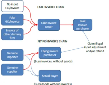
In most cases of VAT evasion, dealers, in their tax-returns, intentionally manipulates the actual state of their business affairs guided with the motivation to pay less amount in tax. Bill trading is used to evade tax [19], in which, a merchant sells the merchandise to a buyer by wilfully avoiding the issue of invoice but collecting the tax. Later, a fake invoice is issued to a third dealer, who can use it to reduce his/her tax burden as shown in Figure 1.2.

Figure 1.2: Bill Trading

To hide the above mentioned manipulations, which can be detected by tax enforcement officers, dealers collude with each other and do heavy illegitimate sales and purchases among themselves without any potentialvalue-addas given in Figure 1.3.

(12)

In Figure 1.3, the transactions represented using thick red-lines going from merchant A to merchant D, merchant A to merchant C and merchant D to merchant C are suspicious transactions. Guided with the motivation of confusing tax authorities, dealers complicate the process by superimposing the illegitimate transactions on the suspicious transaction as represented using thin yellow lines. Note that they superimpose illegitimate transactions such that tax liability of any dealer remains the same,i.e., tax paid on illegitimate purchases is same as the tax collected on illegitimate sales.

Figure 1.3: Circular flow of sales/purchases

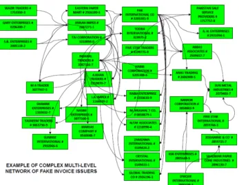
As the value-add due the illegitimate transactions equals zero value, they will not pay any VAT on these transactions (illegitimate transactions), in addition, creating confusion to the tax authorities about the suspicious transactions. Note that colluding dealers do heavy trading among themselves, as compared to trading with the others. This technique of tax evasion technique is known as circular trading [8],[7],[18]. Hence the dealers complicate the process of identifying their suspicious transactions. It is worthwhile to note that few of the fraudulent merchants in circular trading may actually be fictitious (or duplicate) entities formed by fraudulent real dealers. Figure 1.4 shows a real world example of circular trading.

(13)

(14)

Part II

(15)

Chapter 2

Graph Theory and Machine

Learning Terminologies

2.1 Benford Analysis

Benford’s law is a mathematical technique for fraud detection [3],[17],[5] in naturally occurring numerical data sets. Benford’s law, also called as the first digit law, is an observation about the probability distribution of leading digit in naturally occurring numeral data sets. This law states that in many naturally occurring collection of numbers the leading significant digit is likely to be small. Benford’s law also make projection about second digits, third digit, digit combination and so on. This result applies to a variety of data sets including electricity bills, stock prices, house prices, population numbers, death rates, length of rivers, processes described by nature law, etc. We can also use this technique to detect over statements of revenue, fictitious sales and receivables [3].

Benford’s law states that for any numerical data, which is neither purely random nor highly con-straint, the percentage of numbers starting with the digitdfollows the formulalog10(1 + 1/d), where

d ∈ {1,2, ...,9}. Figure 2.1 shows this distribution in pictorial manner. Statistical methods like Goodness-of-fit tests can be used to test if the data’s first digits conform to expected distribution given by above formula. When data did not conform to Benford’s law, a null-hypothesis rejection suggests that some form of manipulation has taken place in the given data set.

(16)

2.1.1 Mean absolute deviation(MAD)

Mean absolute deviation(MAD) is a commonly used statistical measure to test if the data’s first digits conform to expected probability distribution. MAD is calculated as follow

M AD=Pn

i=1(APi−EPi)/n, whereAPidenotes the observed portion of i

th_{bin, and}_EP

i denotes

the expected portion of ith _{bin, and} _n _{is the total number of bins (which is equal to 9 for first}

digit test). Based on the mean absolute deviation value, we can establish the conformity between expected distribution and observed distribution as given below [14].

• Close conformity- MAD is from 0.000 to 0.004

• Acceptable conformity — MAD is from 0.004 to 0.008

• Marginally acceptable conformity — MAD is from 0.008 to 0.012

• Nonconformity — MAD is greater than 0.012

Figure 2.1: Benford’s Law, Logistic Regression

2.2 Machine Learning

Machine learning is commonly divided into three main types:

• Supervised LearningIn this type of learning we are trying to learn a hypothesish:X →y

(17)

Y is finite, we say that the task is aclassification task and if it is continuous we say that it is a regression task.

• Unsupervised Learning If all we have is the input data X and no output data to guide our training, the task is called unsupervised learning. The focus in this type of learning is to discover hidden structure in the data. Common problems in unsupervised learning are dimensionality reduction and clustering of the input data.

• Reinforcement Learning In reinforcement learning we have a situation where the learning algorithm interacts with an environment and is trying to learn how to behave. The cues for whether or not the algorithm is behaving optimally is given only occasionally in the form of (usually) scalar reward values. Reinforcement learning can be viewed as a a form of semi-supervised learning where the training signal is sparse and delayed. It can also be viewed as planning in a domain with stochastic transitions.

2.2.1 Logistic Regression

It’s a classification algorithm, that is used where the response variable is categorical. The idea of Logistic Regression is to find a relationship between features and probability of particular outcome.

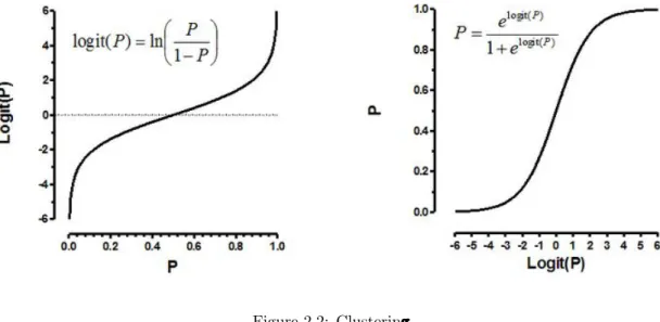
Logistic regression is an estimation of Logit function. Logit function is simply a log of odds in favor of the event. This function creates a s-shaped curve with the probability estimate, which is very similar to the required step wise function. Here goes the first definition :

Logit Function:

(18)

Figure 2.2: Clustering

2.3 Graph Terminology

Graphs are a fundamental construct in complex SNA research, and the use of graph theoretic algorithms and metrics to extract useful information from a social graph is a primary method of analysis in SNA. Formally, a social network is represented as a graph G = (V, E), where V(G), represents the set of vertices, and E(G) refers to the set of edges in the graph (simply V and E

when no ambiguity arises) and both consist of a finite number of elements n=|V| and m =|E|, respectively. The edges in the graph betweenu∈V andv∈V is represented as a pair (u, v)∈E.

2.3.1 Graph clustering

Graph clustering is an unsupervised machine learning algorithm which clusters (groups) the graph nodes, such that most edges are inside individual clusters, and inter-cluster edges are comparatively less [1]. Graph clustering has become a very useful tool for the analysis of graphs in general, with applications ranging from the field of social sciences to biology. Graph clustering algorithms falls under unsupervised learning framework, where algorithm divides the graph into sub graphs with very little guidance from user. Clustering is a well researched topic [4]. Some popular classes of clustering algorithms are geometric, hierarchical and partitioning methods.

There are two types of hierarchical clustering algorithms which are top-down or bottom-up. Bottom-up algorithms treat each node as a singleton cluster at the start of the algorithm and then successively merge (or agglomerate) pairs of clusters which are highly similar until all clusters have been combined

(19)

(20)

Part III

(21)

Chapter 3

Related Works

3.1 Predictive analytics to control fraud

In [25], authors built analytical models to predict tax avoidance by firms. They constructed a social network of firms connected through shared board membership. In [21], authors demonstrated that clients engaging better-connected individual auditors have comparatively lower effective tax rates. Their findings suggest that an environment encouraging individual cross-appointments over multiple engagements can facilitate the transfer of expertise between members of professional teams. In [11], authors investigated whether individual top executives have incremental effects on their firms tax avoidance that cannot be explained by characteristics of the firm. To identify executive effects on a firm’s effective tax rates, they constructed a data set that tracked the movement of 908 executives across the firms over time. Results indicated that individual executives played a significant role in determining the level of tax avoidance that the firms undertake. In [20], authors focused on social security fraud where companies are linked to the resources they use and share. Their aim was to detect fraudulent companies by propagating a time-dependent exposure score for each node based on its relationships to known fraud entities in the network, deriving cliques of companies and resources, and labeling these cliques in terms of their fraud and bankruptcy involvement, and characterizing each company using a combination of intrinsic and relational features and its membership in sus-picious cliques. In [23], authors introduced a new approach, called AFRAID, which utilizes active inference to better detect fraud in time-varying social networks,i.e.,classify nodes as fraudulent vs. non-fraudulent. In [13], authors developed classification models based on Artificial Neural Networks

(22)

(ANN) and Logistic Regression (LR) and applied them on the credit card fraud detection problem. This study is one of the first to compare the performance of ANN and LR methods in credit card fraud detection with a real data set. In [16], author introduced a new fraudulent structure, the so-called spider construction. Focusing on the egonet of each company, the proposed method can handle large scale networks. In order to face the skewed class distribution, the SMOTE approach is applied to re-balance the data. The models were trained on different time stamps and evalu-ated on varying time windows. Using techniques such as Random Forest, Logistic Regression and Naive Bayes, this thesis shows that the combined relational model improves the AUC score and the precision of the predictions in comparison to the base scenario where only local variables are used. In [10], authors focused on auto insurance fraud, which occurs in both auto physical dam-age (APD-collision and comprehensive) and injury claims (Personal Injury Protection-PIP). They looked at various situations within APD and PIP claims and various tactics that insured people use to defraud insurance companies. Then they applied logistic regression as a statistical tool to help identify fraudulent claims. In [12], authors explained a project which was undertaken to improve participation in a rehabilitation program by the patients of the Virga Jesse Hospital’s cardiology department. The probability that a patient joins the program is modeled as a function of a variety of factors based on a data set of 516 patients. The logistic regression model developed by them shows that the major influence factors are the distance from the patient’s home to the hospital and whether or not the patient has a car. This analysis led to several measures to stimulate carpooling.

3.2 Clustering analysis to detect fraud

Several approaches are proposed for detecting circular trading in stock trading. In [8], Palshikar et al. given a graph clustering algorithm which is highly customized for identifying collusion sets in stock market trading. Dempster–Schafer theory was used to merge collusion sets. In [15], Wang, J et al. presented an algorithm to identify the probable collusive sets in an instrument of future markets. They calculated the correlation coefficient among any two aggregated time series. Then they combined the connected components from several highly sparse weighted graphs generated by making use of the correlation matrices. In [9], Islam, N.Md. et al. had given a Markov Clustering algorithm for finding collusion sets. Their approach can identify both purely circular collusion sets and cross trading collusion sets. MCL was used by them at different strength of residual value to identify various clusters from stock flow graph. Traditional centrality measures for graphs are

(23)

capable to identify the kingpins and their proxies. These functions give very minimal information in huge and diverse networks. Generally, the central players of the graph (usually too many) are not highly associated to a group of actors of interest, such as a group of drug traders or fraudsters. In [22], Vicente, E. et al. gave complicity functions(measures), which are capable to identify the intermediaries, avoiding central actors who are not related to this group. These functions are able to identify a set of fraudsters according to the strength of their association with the others to facilitate the identification of organized crime rings. In [13], Nigrini Mark J. et al. defined several digit and number tests which can be used by charted accountants as statistical methods in the starting stages of the audit. The mathematical foundation of these tests is the Benford’s law, a specific property of tabulated numbers that gives the expected probability of the digits in tabulated data. Many experimental studies suggested that the digit patterns of genuine numbers follows the expected probability distribution of Benford’s law. Thus, auditors could test the reliability of list of numbers by comparing the actual and expected distribution. In [14], Arben Asllani et al. gave a template which can be used by charted accountants to detect fraud in accounting practices. This template is based on the Benford’s Law. They illustrated the use of this method by taking example from a local Albanian hospital. Their investigation leads to very important findings and demonstrate the usefulness of this approach. In [5], Durtschi et al. identified data sets which follows Benford’s law, discussed the power of different statistical testing procedures, various types of frauds which can be identified and cannot be identified by such analysis, the potential problems which arise when an account contains too few observation. An actual example is provided to demonstrate where Benford’s law is successful in identifying fraud in population of accounting data.

(24)

Part IV

(25)

Chapter 4

Thesis Contributions

4.1 Predictive Modeling for Identifying Return Defaulters

Our objective is to build a predictive model which will help tax officials to predict whether a given firm (business entity) will file GST return or not in the coming month. We built this model based on the firm’s past returns filing behaviour, volume of business, value of interactions with the other firms andMADvalue of the first digit Benford’s analysis on the sales transactions of this firm. We developed this model for the commercial taxes department of Telangana, India. For the same, we used the data set provided by them that contains two main tables.

4.1.1 Dataset

4.1.1.1 Way-Bill Data

Following table contains some fields of way-bill data. Way-bill is a necessary document to be carried when goods are being transported from one place to the other. Every movement of goods needs a unique way-bill. Each row in the Table 4.1 corresponds to a way-bill generated online.

Actual database system contains additional information, such as, tax rate, quantity of goods sold, vehicle used for transportation, etc. Note that, each record in the above given table refers to one sales/purchase transaction between a seller and a buyer. The data set we used contains few million rows of such transactions.

(26)

S. No. Seller Buyer Time Amount(Rs) 1 Merchant X Merchant Y 2018/02/04/14:30 12000 2 Merchant Z Merchant U 2018/02/04/16:01 18000 3 Merchant X Merchant U 2018/02/05/18:10 14000 4 Merchant Y Merchant Z 2018/02/05/16:12 15000 5 Merchant Z Merchant X 2018/02/05/14:03 12000

Table 4.1: WAY-BILL DATA

4.1.1.2 GST Return Data

Following table contains some fields of GST returns data. Actual database system contains additional

S.No. Firm Month Purchases ITC Sales Output Tax

1 A July-17 100000 18000 200000 36000

2 A Aug-17 300000 48000 500000 90000

3 B Sep-17 200000 36000 300000 48000

Table 4.2: GST RETURNS DATA

information, like, method of payment of tax, date of filing, exports value, exempted sales, zero rated sales and sales on reverse charge mechanism.

4.1.2 Building the Network of Firms

We created a weighted directed graph. Each node(vertex) in this graph corresponds to a firm. Weight of a node is the average tax paid per month [ATPM] by the firm during the period July-2017 to December-2017. We performed min-max normalization on the vertex weights and outlier cleansing as there were few firms whoseATPM was far higher than the rest. We used the data in Table 4.2 towards this. We coloured each node eitherREDorGREEN.REDmeans that the firm did not file at least one GST return, while GREEN means that the firm had filed all the GST returns. This can be achieved using the data in Table 4.2. We placed a weighted directed edge from firm A to firmB, where edge weight is the amount of sales done by firmAto firmBduring the financial year 2016-2017. We performed min-max normalization of edge weights, and outlier cleansing as some way-bill values were quite high due to typing mistakes. For the same, we used the data in Table 4.1. This network helps in understanding the flow of information between firms.

(27)

4.1.3 Feature Extraction

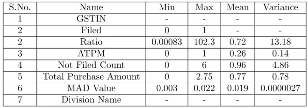
We constructed a data set with columns(variable) mentioned in Table 4.3. Note that each row of this data set corresponds to a firm. No. of rows in the data set is 58,154.

S.No. Name Min Max Mean Variance

1 GSTIN - - -

-2 Filed 0 1 -

-2 Ratio 0.00083 102.3 0.72 13.18

3 ATPM 0 1 0.26 0.14

4 Not Filed Count 0 6 0.96 4.86

5 Total Purchase Amount 0 2.75 0.77 0.78

6 MAD Value 0.003 0.022 0.019 0.0000027

7 Division Name - - -

-Table 4.3: Features

LetRdenote all the red coloured vertices in the social network explained in subsection 4.1.2 andG

denote all the green coloured vertices. Letabe the vertex for which we are extracting the features. Below we will provide the explanation for each variable (feature) mentioned in the Table 4.3.

GSTIN: GST identification number of firm a. It is a 15 characters string given at the time of the registration of the firm.

Filed: GST return filing status(filed/not filed) of firmafor the month Jan-2108. We denoted filed with ‘1’ and not filed with ‘0’. This is the dependent variable. Note that, in the data set there are 73.3% class 1 records and rest are class 0 records.

Not Filed Count: This is the number of GST returns not filed byafrom July-2107 to December-2017.

Division-Name: Telangana state, India, is divided into twelve geographic divisions for adminis-trative purposes. This variable is the name of the division whereais located.

Ratio: This is a feature extracted from the social network that we explained in subsection 4.1.2. It captures the information flow between firma and other firms. Indirectly this also captures the influence of other firms on firm a. Ifa has close ties with firms which are not filing GST returns, then, they would influenceato not to file GST return and vice-verse.

• a11 = Pv∈R

w(v)∗w(va)

w(v)+w(va), where w(v) is the weight of vertex v and w(va) is the weight of directed edge va

(28)

• a21 = P_v_∈_G_ww₍(_vv₎₊)∗w_w(₍va_va)₎, where w(v) is the weight of vertex v and w(va) is the weight of directed edge va

• a22=Pv∈G

w(v)∗w(av)

w(v)+w(av).

Then the value of Ratio for vertex a is _aa11+₂₁₊a_a12₂₂. More the value of Ratio meansa is doing more business with return defaulters who can influence a to not to file tax return. Figure 4.1 explains the relation between Ratiovariable and Log of Odds of dependent variableFiled. Note that Log of Odds of dependent variableFiledis decreasing asymptotically. So, in our model we use log ofRatio as an independent variable.

Figure 4.1: Ratio Vs Log of Odds

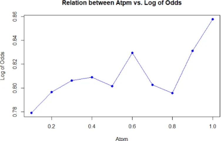
ATPM: This is the weight of vertex a. Figure 4.2 explains the relation between ATPM variable and Log of Odds of dependent variableFiled. The relation is a polynomial relation. So, we included square, cube and square root ofATPMin the model.

Total Purchase Amount: It is the total amount of purchases made by a in lakhs (1 lakh = 100,000) of rupees. Figure 4.3 explains the relation betweenTotal Purchase Valueand Log of Odds of dependent variableFiled. This relation is a linear relation.

MAD Value: Mean absolute deviation value of the first digit Benford’s analysis on sales trans-actions of a. Figure 4.4 explains the relation between MAD Value and Log of Odds of dependent variableFiled. This relation is a non-linear relation.

(29)

Figure 4.2: ATPM Vs Log of Odds

Figure 4.3: Total Purchase Vs Log of Odds

4.1.4 Experimental Results

4.1.5 Model Parametric Coefficients

We built logistic regression model inR[2] [6]. Figure 4.5 gives the parametric coefficients.

Telangana state is divided into twelve geographic divisions for administrative purpose. From Figure 4.6, one can infer that the distribution ofATPMis not the same across all the divisions. To capture this information, we created interaction variables by multiplying dummy variables corresponding to Division NamesandATPM. We observed that even though there are twelve divisions in Telangana, interaction between only two divisions andATPMis statistically significant. Variables 13 and 14 in Table 4.5 are these two interaction variables.

(30)

Figure 4.4: MAD Value Vs Log of Odds

Figure 4.5: Parametric Coefficients

Figure 4.6: Division Vs ATPM

Note that variable 2 in Table 4.5 is the logarithmic value ofRatio. This is taken because the observed relation between the log of odds of dependent variable Filed and Ratio as shown in Figure 4.1 is

(31)

logarithmic in nature. We took the square, cube and square-root values of ATPM because the observed relation between log of odds of dependent variable Filed and ATPM as shown in Figure 4.2 is a polynomial relation of degree greater than three. Note that the relation between log of odds of dependent variable Filedand Total Purchase Value as shown in Figure 4.3 is a linear relation. Square and cube values ofMAD Valueare taken because the observed relation between log of odds of dependent variableFiledandMAD Valueas shown in Figure 4.4 is a polynomial relation of degree greater than three.

4.1.6 Model Performance

Training accuracy of the model at the cutoff equal to 0.5 is 86.38% and testing accuracy is 86.33%. Precision of the model is 85.5%. Recall of the model is 97.97%. From the confusion matrices given in Figure 4.7 and Figure 4.8, one can observe that almost all class 1 records are correctly classified and 54% of class 0 records are correctly classified.

Figure 4.7: Training Confusion Matrix

Figure 4.8: Testing Confusion Matrix

4.1.6.1 Concordance Measure

Total number of pairs are 59416312. Concordance value is 0.8119749 and discordance value is 0.1880251.

4.1.6.2 ROC curve

As given in Figure 4.9 and Figure 4.10, the area under the training ROC curve is 0.814 and the testing ROC curve is 0.812. Since the area under both the curves are almost the same, one can conclude that the model is not over fitting. Since the area under the training ROC curve is more than 0.7, one can say that model is not under fitting.

(32)

Figure 4.9: Training ROC Curve

Figure 4.10: Testing ROC Curve

4.1.6.3 Log Likelihood Chi-square Test

The log likelihood chi-square test is a test to see if the model as a whole is statistically significant. It is 2 times the difference between the log likelihood of the current model and the log likelihood of the intercept-only model. Deviance scores of the model are given in Figure 4.11. Thepvalue ofLog Likelihoodtest is almost zero.

(33)

4.1.6.4 Lift Chart

Lift is a measure of the effectiveness of a predictive model calculated as the ratio between the results obtained with and without the predictive model. Figure 4.12 is the lift chart for the proposed model.

Figure 4.12: Lift Chart

4.2 Collusion Set detection using Graph Clustering [24]

4.2.1 Sales flow graph

Using the sales and purchase database, we constructed a weighted directed graph, denoted byGs=

(V, E), where V is the set of weighted vertices (each vertex is uniquely identified by a dealer ID), andE is the set of weighted directed edges. We call this graph assales flow graph.

4.2.1.1 Assigning weights to edges

Letlbe the number of sales transactions from dealer (node)ato dealer (node)bandv1, v2, v3, . . . , vl

be values of these sales transactions. Let φ(ab) be the mean absolute deviation value of first digit Benford’s analysis onv1, v2, v3, . . . , vl. Based on the value ofφ(ab), we can establish the conformity

between expected distribution and observed distribution.

The weight of edge froma tob is given by (l∗Pl

i=1vi∗1000φ(ab))/(l+P l

i=1vi). Note that edge

weight increases in an exponential manner with the increase in φ(ab), i.e., lesser the conformity between expected distribution and observed distribution, then more weight is assigned to the edge. Lesser the number of transactions or sum of values of transaction, then lesser edge weight is assigned to the edge [1].

(34)

4.2.1.2 Assigning weights to vertices

Let m be the number of sales and purchase transactions by dealer a and v1, v2, v3, . . . , vm be the

values of these transactions. Letφ(a) be the mean absolute deviation value of the first digit Benford’s analysis onv1, v2, v3, . . . , vm. Weight of vertexais given by (m∗P

m

i=1vi∗100φ(a))/(m+P m i=1vi).

4.2.2 Graph clustering

Graph clustering is an unsupervised machine learning algorithm which clusters (groups) the graph nodes, such that most edges are inside individual clusters, and inter-cluster edges are comparatively less [1]. Graph clustering has become a very useful tool for the analysis of graphs in general, with applications ranging from the field of social sciences to biology. Graph clustering algorithms falls under unsupervised learning framework, where algorithm divides the graph into sub graphs with very little guidance from user. Clustering is a well researched topic [4]. Some popular classes of clustering algorithms are geometric, hierarchical and partitioning methods.

There are two types of hierarchical clustering algorithms which are top-down or bottom-up. Bottom-up algorithms treat each node as a singleton cluster at the start of the algorithm and then successively merge (or agglomerate) pairs of clusters which are highly similar until all clusters have been combined into a single cluster [19].

4.2.3 Detecting and Managing Outliers

In Benford’s analysis, the probability of nine being the first digit is log10(1 + 1/9) = 0.046. So we need atleast twenty two sales transactions between any two dealers so that expected number of sales transaction withninebeing the first digit is atleast one. As part of data cleansing, we remove any edge between a pair of dealers (vertices) if the number of sales transactions between them is less than twenty two. In the same manner, we remove any dealer if the number of sales/purchase transactions by this dealer is less than twenty two.

If the weight of any edge is more than the median of edge weights plus 1.5 times the interquartile range of edge weights, then replace this edge weight by median of edge weights plus 1.5 times the interquartile range of edge weights. Similarly, if the weight of any vertex is more than themedian of vertex weights plus 1.5 times the interquartile range of vertex weightsthen replace this vertex weight bymedian of vertex weights plus 1.5 times the interquartile range of vertex weights[19].

(35)

4.2.4 Similarity measure between clusters

LetS1, S2be two disjoint set of vertices. Letα(S1, S2) be defined assum of weights of all edges f rom S_|_S_1|∗|_S_2| 1 to S2. Letγ(S1) is defined as sum of weights of all vertices in S1

|S1|

Proximity (or similarity) score between any two disjoint set of vertices, say set A and set B, is defined asβ(A, B) = (_αα₍(_ABAB₎₊)∗α_α(₍BA_BA)₎)∗(_γγ₍(_AA₎₊)∗γ_γ(₍B_B)₎). We give high proximity score ifAandBsatisfies the following conditions:

• Sum of the edge weights from AtoB is large

• Sum of the edge weights from B toAis large

• Average weight of vertices inAis large

• Average weight of vertices inB is large

Proximity score between three disjoint set of verticesA,BandCis defined asβ(A, B, C) =max(min(

α(AB)∗α(BC) α(AB)+α(BC), α(BC)∗α(CA) α(BC)+α(CA), α(CA)∗α(AB) α(CA)+α(AB)), min( α(AC)∗α(CB) α(AC)+α(CB), α(CB)∗α(BA) α(CB)+α(BA), α(BA)∗α(AC) α(BA)+α(AC)))*min( γ(A)∗γ(B) γ(A)+γ(B), γ(B)∗γ(C) γ(B)+γ(C), γ(C)∗γ(A) γ(C)+γ(A))

4.2.5 Algorithm

We use hierarchical clustering with bottom-up approach. We use the proximity measure defined in subsection 4.2.4 to find the similarity between clusters. From our experimental study on sale flow graphs we observed that any cluster in sales flow graph contains a lot of cycles of length two and three. We also observed that the number of dealers in any colluding set is less than or equal to eight in almost all cases. That is the reason we merge two or three disjoint clusters in any iteration of

Algorithm1.

In the following subsection, we give a brief overview on the running of the algorithm. As evident in the following, one can find the clusters to be merged in polynomial time by using the max heap implementation of priority queue.

4.2.6 Time Complexity

Letv denote the number of vertices in the input graph. Every time thewhileloop executes, size of

(36)

Data: Sales flow graphG

Result: Clusters of colluding dealers Perform outlier cleansing;

# This is explained in subsection 4.2.3; Letv1, v2, . . . , vn be the set of vertices inG;

For(i = 1 to n){

ci =vi}

# Each vertex is a cluster of size one; C={c1, c2, . . . , cn}

Let ci, cj be two distinct elements of C such that p1=β(ci, cj) is maximum;

Let ck, cl, cm be three distinct elements of C such that p2=β(ck, cl, cm) is maximum;

pnew=max(p1, p2);

pold=max(p1, p2);

while (pold−pnew is insignificant) do

Let ci, cj be two distinct elements of C such that p1=β(ci, cj) is maximum;

Let ck, cl, cm be three distinct elements of C such that p2=β(ck, cl, cm) is

maximum;

if (p1≥p2) then

Remove ci, cj from C and add ci∪cj to C;

pold=pnew;

pnew=p1;

end else

Remove ck, cl, cm from C and add ck∪cl∪cm to C;

pold=pnew;

pnew=p2; end

end }

Algorithm 1:Clustering algorithm

whileloop we select two or three elements fromC and insert one element. This takesO(logv∗v2₎ time if we use the heap implementation of priority queues for the proximity measures of all possible three element combinations and two element combinations of C. Hence the total asymptotic time taken to run thewhileloop isO(v3_logv_).

4.2.7 Case study

After executing the proposed clustering algorithm we got several clusters. Here we have taken two such clusters and done an in-depth analysis.

(37)

4.2.7.1 Case One

In this cluster four merchants are performing circular trading between them. Figure 4.13 presents the specifics of this circular trading. Note that each edge shows the amount of sales in lakhs, where one lakh equals to 0.10 million currencies. This cluster is a classic example for flying invoice (bill trading). One retailer in this cluster is doing heavy cash sales without issuing invoices to customers and giving fake invoice to a manufacturer in this cluster. This manufacturer uses these fake invoices to minimize his tax liability.

Figure 4.13: case study 1

4.2.7.2 Case Two

In this cluster, eight dealers are practicing huge circular trading between them. Figure 4.14 illustrates the same. This cluster is an example of how dealers misuse the governmental subsidies.

(38)

(39)

Chapter 5

Conclusion and Future Work

We built a binary-regression model that predicts whether a business dealer is a plausible return defaulter or not for the upcoming month. We built the model by exploiting the dealer’s business behavior with other dealers who are either return defaulters or not. We were able to achieve a prediction accuracy of around 87% for our model. In this model we did not include the mis-classification costs. Cost of misclassifying a genuine dealer as a return defaulter is only a few Rupees. However, misclassifying a return defaulter as a genuine dealer will cost a lot of money. In the future, we would like to incorporate mis-classification costs for model building. In addition, we are working towards the development of a network ranking algorithm that ranks the dealers based on their probability to commit tax evasion.

We also studied an important and a highly used technique for evading tax in VAT system known as circular trading. Circular trading is a notorious practice where a group of merchants perform huge illegitimate trade transactions in a circular manner between them in a relatively less amount of time producing no value addition. Identifying the colluding dealers is significant since it aids tax enforcement officers to pin-point the suspicious transactions. Here, we proposed a graph clustering algorithm to identify the colluding dealers. In future, we plan to investigate towards finding other useful methods to identify the colluding dealers. We are also exploring for an algorithm with a better time complexity.

(40)

References

[1] E. A. Patrick R. A. Jarvis. “Clustering using a similarity measure based on shared near-est neighbors”. In: IEEE TRANSACTIONS ON COMPUTERS VOL.C-22,NO. 11 (1973), pp. 1025–1034.

[2] Ross Ihaka and Robert Gentleman. “R: A Language for Data Analysis and Graphics”. In: Journal of Computational and Graphical Statistics 5 (Sept. 1996), pp. 299–314.

[3] Mittermaier Linda J. Nigrini Mark J. “The Use of Benford’s Law as an Aid in Analytical Procedures”. In:Auditing: A journal of practice theory 41 (1997), p. 52.

[4] P.J.Flynn A K Jain M N Murty. “Data Clustering:A Review”. In: ACM Computing Surveys (CSUR) Volume 31 Issue 3 (1999), pp. 264–323.

[5] William Pacini Durtschi Cindy Hillison. “The Effective Use of Benford’s Law to Assist in Detecting Fraud in Accounting Data”. In:Journal of Forensic Accounting Vol.V(2004) (2004), pp. 17–34.

[6] Simon N. Wood, ed. Generalized Additive Models: An Introduction With R. Boca Raton, Fl.:Chapman and Hall/CRC Press, Jan. 2006.

[7] M. Franke, B. Hoser, and J. Schr¨oder. “On the analysis of irregular stock market trading behavior”. In: Data Analysis, Machine Learning and Applications. ISBN: 978-3-540-78239-1,

URL:https://link.springer.com/chapter/10.1007/978-3-540-78246-9_42. Springer,

Jan. 2007, pp. 355–362.

[8] G.K. Palshikar and M.M. Apte. “Collusion set detection using graph clustering”. In: Data Mining and Knowledge Discovery. ISSN: 1384-5810, URL: https : / / link . springer . com / article/10.1007/s10618-007-0076-8. Springer, Apr. 2008, pp. 135–164.

[9] N.Md. Islam et al. “An approach to improve collusion set detection using MCL algorithm”. In: Computers and Information Technology. ISBN: 978-1-4244-6284-1, URL:http://ieeexplore. ieee.org/abstract/document/5407133/. IEEE, Dec. 2009, pp. 237–242.

(41)

[10] J. Holton Wilson. “An Analytical Approach To Detecting Insurance Fraud Using Logistic Regression”. In:Journal of Finance Accountancy Vol. 1 (Aug. 2009).

[11] Scott D. Dyreng, Michelle Hanlon, and Edward L. Maydew. “The Effects of Executives on Corporate Tax Avoidance”. In:The Accounting Review 85 (2010), pp. 1163–1189.

[12] Frank van der Meulen, Thijs Vermaat, and Pieter Willems. “Case Study: An Application of Logistic Regression in a Six Sigma Project in Health Care”. In:Quality Engineering23 (2011), pp. 113–124.

[13] Yusuf Sahin and Ekrem Duman. “Detecting credit card fraud by ANN and logistic regression”. In: 2011 International Symposium on Innovations in Intelligent Systems and Applications. ISBN: 978-1-61284-919-5. IEEE, June 2011.

[14] Joseph T. Wells Mark Nigrini, ed. Benford’s Law: Applications for Forensic Accounting, Au-diting, and Fraud Detection. ISBN: 978-1-118-15285-0. Wiley, Mar. 2012.

[15] J. Wang, S. Zhou, and J. Guan. “Detecting potential collusive cliques in futures markets based on trading behaviors from real data”. In:Neurocomputing 92 (2012), pp. 44–53.

[16] V´eronique Van Vlasselaer et al. “Using Social Network Knowledge for Detecting Spider Con-structions in Social Security Fraud”. In: 2013 IEEE/ACM International Conference on Ad-vances in Social Networks Analysis and Mining. ISBN: 978-1-4503-2240-9. IEEE, Aug. 2013, pp. 813–820.

[17] Manjola Naco Arben Asllani. “Using Benford’s Law for Fraud Detection in Accounting Prac-tices”. In:Journal of Social Science Studies 1 (2014), pp. 129–143.

[18] K. Golmohammadi, O.R. Zaiane, and D. D´ıaz. “ Detecting stock market manipulation using supervised learning algorithms”. In:Data Science and Advanced Analytics. ISBN: 978-1-4799-6991-3 , URL: http : / / ieeexplore . ieee . org / document / 7058109/. IEEE, Nov. 2014, pp. 435–441.

[19] B. Baesens, V.V. Vlasselaer, and W. Verbeke, eds. Fraud Analytics Using Descriptive, Pre-dictive, and Social Network Techniques: A Guide to Data Science for Fraud Detection. ISBN: 978-1-119-13312-4. Wiley, Aug. 2015.

[20] V´eronique Van Vlasselaer et al. “Guilt-by-Constellation: Fraud Detection by Suspicious Clique Memberships”. In: 48th Hawaii International Conference on System Sciences HICSS. ISBN: 978-1-4799-7367-5, URL: DOI: 10.1109/HICSS.2015.114. IEEE, Jan. 2015, pp. 918–927. [21] Bianchi et al. “Professional Networks and Client Tax Avoidance: Evidence from the Italian

(42)

[22] E. Vicente, A. Mateos, and A. Jim´enez-Mart´ın. “Detecting stock market manipulation using supervised learning algorithms”. In:Modeling Decisions for Artificial Intelligence. ISBN: 978-3-319-45655-3, URL: https://link.springer.com/chapter/10.1007/978-3-319-45656-0_17. Springer, Sept. 2016, pp. 205–216.

[23] Veronique Van Vlasselaer et al. “AFRAID: Fraud detection via active inference in time-evolving social networks”. In: 2015 IEEE/ACM International Conference on Advances in Social

Net-works Analysis and Mining (ASONAM). ISBN: 978-1-4503-3854-7, URL: DOI: 10.1145/2808797.2810058. IEEE, Aug. 2016, pp. 659–666.

[24] Priya Mehta et al. “A Graph Theoretical Approach for Identifying Fraudulent Transactions in Circular Trading”. In: DATA ANALYTICS 2017, The Sixth International Conference on Data Analytics. Nov. 2017.

[25] Jasmien Lismont et al. “Predicting tax avoidance by means of social network analytics”. In: Decision Support Systems 108 (2018), pp. 13–24.

Predictive Analytics For Controlling Tax Evasion