Macroeconomic effects of simultaneous
implementation of reforms after the crisis
A. Gerali, A. Notarpietro, M. Pisani
∗May 26, 2015
Abstract
This paper evaluates the macroeconomic effects of simultaneously implementing fiscal consolidation and competition-friendly reforms in a country of the euro area by simulating a large-scale dynamic general equilibrium model. We find, first, that the joint implementation of reforms has additional expansionary effects on long-run economic activity. Increasing competition in the service sector favors a higher income tax base. Given the targeted public debt-to-GDP ratio, labor and capital income tax rates can be reduced by more than with fiscal consolidation alone. Second, fiscal consolidation has non-negligible medium-run costs; however, they are reduced by joint implementation with the services reform.
JEL classification: C51; E30; E63
Keywords: Competition; Fiscal Policy; Markups; Monetary Policy; Public Debt; Spread.
∗Bank of Italy, Modelling and Forecasting Division. The views expressed in this paper are those of the authors alone and should not be attributed to the Bank of Italy. We thank Alberto Locarno, Giuseppe Ferrero, Henrik Kucsera, Eva Ortega, Mate Toth, two anonymous referees and participants at 2014 Economic Society Conference; Magyar Nemzeti Bank 12th Macroeconomic Policy Research Workshop on Growth, Rebalancing and Macroeco-nomic Adjustment after Large Shocks, Bank of Italy seminar, Working Group on Econometric Modelling of the European System of Central Bank (2014), 2014 Central Bank Macroeconomic Modelling Workshop. Correspon-dence: [email protected], [email protected], [email protected]
Fiscal consolidation should be designed in a growth friendly manner while struc-tural reforms will boost potential growth.
European Central Bank President Mario Draghi, Hearing at the Committee on Eco-nomic and Monetary Affairs of the European Parliament, Brussels, 3 March 2014.
1
Introduction
Two legacies of the recent European sovereign crisis are the high level of public debt and the persistently weak economic performance.1 They will probably condition the European economic
outlook for several years to come and are closely related. Public debt consolidation should be achieved by limiting the increase in tax rates, which could further jeopardize European economic performance.2
At the same time, restoring high economic growth helps to increase the tax base and, hence, to contain the increase in tax rates needed to improve public finances.
The close connection between public debt sustainability and growth performance calls for the appropriate set of policies to be found, in particular, and crucially, for possible synergies across policies to foster a structural (supply-side) improvement of the European economy.
This paper evaluates the macroeconomic effects of simultaneously implementing growth-friendly fiscal consolidation and competition-growth-friendly reforms in one European country by simu-lating a large-scale dynamic general equilibrium model.
The assessment is based on simulating a three-country large-scale new-Keynesian dynamic general equilibrium model of one country in the euro area (labelled “Home”), the rest of the euro area (REA) and the rest of the world (RW) economy, akin to the Eurosystem EAGLE (Euro Area and Global Economy model, see Gomes et al., 2010).3 The euro area (EA) is a two-region
monetary union and therefore has a common monetary policy and nominal exchange rate against
1
The views expressed in this paper are those of the authors alone and should not be attributed to the Bank of Italy. We thank Alberto Locarno, Giuseppe Ferrero, Henrik Kucsera, Eva Ortega, M´at´e T´oth, two anonymous referees and participants at 2014 Royal Economic Society Conference; Magyar Nemzeti Bank 12th Macroeconomic Policy Research Workshop on Growth, Rebalancing and Macroeconomic Adjustment after Large Shocks, Bank of Italy seminar, Working Group on Econometric Modelling of the European System of Central Bank (2014), 2014 Central Bank Macroeconomic Modelling Workshop.
2
According to the Europe 2020 Strategy “raising taxes on labour, as has occurred in the past at great costs to jobs, should be avoided”. See European Commission (2010).
3
See also the Global Economic Model developed at the International Monetary Fund (see Laxton and Pesenti 2003 and Pesenti 2008) and the New Area Wide Model developed at the European Central Bank (see Christoffel et al., 2008 and Coenen et al., 2008).
the RW block (the latter has its own monetary policy and currency). The model features country-specific public sectors and monopolistic competition in product and labor markets. The public sector has lump-sum transfers and public consumption on the expenditure side and, crucially, (distortionary) taxes on labor income, capital income and consumption on the revenue side. Public debt is stabilized through a fiscal rule, that accordingly sets one of the available fiscal items to hit the public debt target and stabilize the public deficit. Monopolistic competition in the product (labor) market is formalized by a mark-up between the marginal cost (marginal rate of substitution between consumption and leisure) and prices (wages). In this framework, mark-ups are inversely related to the degree of substitutability across product and labor varieties, and hence the underlying level of competition. Given the presence of nontradables, we can analyze the effects of increasing the degree of competition in the service sector, traditionally considered mainly nontradable. Finally, the inclusion of the RW allows for a full characterization of trade flows. All simulations are run under the assumption of perfect foresight. As such, fiscal and competition-friendly reforms are fully credible, there is no uncertainty and households and firms anticipate the transition paths and the final equilibria.
We initially simulate fiscal consolidation strategies based on labor or, alternatively, capital income taxes to permanently reduce the public debt-to-(annualized) GDP ratio by 10 percentage points over a ten-year period. This means that, in the case of labor (capital) income tax-based consolidation, the adjusted instrument in the fiscal rule is the labor (capital) tax rate. Initially the rule commands an increase in labor (capital) tax rate. As the reduction in the debt-to-GDP ratio and in the implied interest payment progress, new fiscal room is created to actually reduce tax rates. The resulting path of tax rates is typically hump-shaped and the consolidation ends up by reducing the labor (capital) tax rate on a permanent basis.
Next, we evaluate the macroeconomic impact of competition friendly-reforms in the service sector. The sector-specific (gross) mark-up is gradually reduced by 5 percentage points over a ten-year-period. The effects of the reform are evaluated first in isolation and then, crucially for the goal of this paper, combined with the consolidation of public debt.
Our results are as follows.
jointly implemented with the labor income tax based and capital income tax based consolidation, respectively. GDP increases by 0.3 and 1.2 percent respectively of the initial level in the case of labor income and capital income tax based consolidations implemented in isolation. Similarly, the increase in the service sector competition favors the increase in GDP by 1.3 percent. The joint implementation of public debt consolidation and competition reform has further, additional expansionary effects. Indeed, increasing competition in the service sector has not only a positive direct effect on output but also an indirect one. The higher output implies a higher labor income and capital income tax base. For a given target of the public debt-to-GDP ratio, in the long run it is possible to reduce the tax rates by more than with isolated fiscal consolidation. The additional reduction in taxation further stimulates economic activity.
Second, in the medium run the output loss, associated with the temporary increase in taxes during the consolidation, is partly mitigated by the joint implementation with the services reform. Competition-friendly reforms partially counterbalance the recessionary effects of the increase in tax rates, limiting the decrease in the income tax base. This makes it possible to limit the increase in tax rates needed to reduce public debt.
Our paper is related to several contributions in the literature. Forni et al. (2010a, b) and Lusinyan and Muir (2013) evaluate the macroeconomic impact of structural reforms and fiscal consolidation in Italy. Gomes et al. (2013) evaluate the macroeconomic impact of enhancing competition in the German labor market and service sector. Unlike these papers, we analyze the interaction between structural reform in the service sector and fiscal consolidation. Synergies across policies are also analyzed by Fiori et al. (2012). They investigate the effect of product market liberalisation on employment and consider possible interactions between policies and institutional changes in product and labour markets. Our contribution focuses on the interaction between fiscal consolidation and liberalisation.
The paper is organized as follows. Section 2 reports the main theoretical features of the model setup and the calibration. In particular, it shows equations of the fiscal sector, the imperfect competition regime in the service sector, the formalization of sovereign spread and ZLB. Section 3 reports the main results of implementing the reforms. Section 4 concludes.
2
The model
An overview of the model is initially reported. Subsequently, the crucial features for the simu-lations are illustrated, i.e. how taxes, monopolistic competition, sovereign spread and monetary policy rate affect choices of households. Finally, the calibration is reported.
2.1
Overview
The model represents a world economy composed by three regions: Home, REA and RW. In each region there is a continuum of symmetric households and symmetric firms. Home households are indexed by j ∈ [0;s], households in the REA by j∗
∈ (s;S], households in the RW by
j∗∗
∈(S; 1].4
Home and the REA share the currency and the monetary authority. The latter sets the nominal interest rate according to EA-wide variables. The presence of the RW outside the EA allows to assess the role of the nominal exchange rate and extra-EA trade. In each region there are households and firms. Households consume a final good, which is a composite of intermediate nontradable and tradable goods. The latter are domestically produced or imported. Households trade a one-period nominal bond, denominated in euro. They also own domestic firms and use another final good (different from the final consumption good) to invest in physical capital. The latter is rented to domestic firms in a perfectly competitive market. All households supply differentiated labor services to domestic firms and act as wage setters in monopolistically competitive labor markets by charging a mark-up over their marginal rate of substitution between consumption and leisure.
On the production side, there are perfectly competitive firms that produce two final goods (consumption and investment goods) and monopolistic firms that produce intermediate goods. The two final goods are sold domestically and are produced combining all available intermediate goods using a constant-elasticity-of-substitution (CES) production function. The two resulting bundles can have different composition. Intermediate tradable and nontradable goods are
pro-4
The parametersis the size of the Home population, which is also equal to the number of firms in each Home sector (final nontradable, intermediate tradable and intermediate nontradable). Similar assumptions holds for the REA and the RW.
duced combining domestic capital and labor, that are assumed to be mobile across sectors. Intermediate tradable goods can be sold domestically and abroad. Because intermediate goods are differentiated, firms have market power and restrict output to create excess profits. We also assume that markets for tradable goods are segmented, so that firms can set three different prices, one for each market. In line with other dynamic general equilibrium models of the EA (see, among the others, Christoffel et al. 2008 and Gomes et al. 2010), we include adjustment costs on real and nominal variables, ensuring that, in response to a shock, consumption, pro-duction and prices react in a gradual way. On the real side, habit preferences and quadratic costs prolong the adjustment of households consumption and investment, respectively. On the nominal side, quadratic costs make wages and prices sticky.5
2.2
Public debt consolidation and tax rates
Public debt consolidation affects households’ choices through the implied change in the tax rates. Fiscal policy is set at the regional level. The government budget constraint is:
Btg+1
RH t
−Btg≤(1 +τc
t)PN,tCtg+T rt−Tt (1)
where Btg ≥0 is nominal public debt. It is a one-period nominal bond issued in the EA-wide market that pays the gross nominal interest rate RH
t . The variable C g
t represents government
purchases of goods and services, T rt > 0 (< 0) are lump-sum transfers (lump-sum taxes) to
households. Consistent with the empirical evidence,Ctg is fully biased towards the intermediate
nontradable good. Hence it is multiplied by the corresponding price indexPN,t.6
We assume that the same tax rates apply to every household. Total government revenues
Ttfrom distortionary taxation are given by the following identity for the case of Home (similar
expressions hold for REA and RW):
Tt≡ Z s 0 τtℓWt(j)Lt(j) +τtk RktKt−1(j) + ΠPt (j) +τtcPtCt(j)dj−τtcPN,tCtg (2) whereτℓ
t is the tax rate on individual labor incomeWt(j)Lt(j),τtkon capital incomeRktKt−1(j)+
5
See Rotemberg (1982).
6
ΠP
t (j) andτtcon consumptionCt(j). The variableWt(j) represents the individual nominal wage,
Lt(j) is individual amount of hours worked,Rkt is the rental rate of existing physical capital stock
Kt−1(j), ΠPt (j) stands for dividends from ownership of domestic monopolistic firms (they are
equally shared across households) andPt is the price of the consumption bundle.
The government follows a fiscal rule defined on a single fiscal instrument to bring the public debt as a percent of domestic GDP,bg>0, in line with its target ¯bgand to limit the increase in
public deficit as ratio to GDP (bgt/b g t−1): 7 it it−1 = bgt ¯ bg φ1 bgt bgt−1 φ2 (4)
where it is one of the five fiscal instruments among three tax rates (τtℓ, τtk, τtc) and the two
expenditure items (Ctg, T rt). Parametersφ1, φ2 are lower than zero when the rule is defined on
an expenditure item, calling for a reduction in expenditures whenever the debt level is above target and for a larger reduction whenever the dynamics of the debt is not converging. To the contrary, they are greater than zero when the rule is on tax rates.
The simulation of Home fiscal consolidations implies that the target on government debt, ¯bg, is gradually and permanently reduced. The adjusted instrument is the labor income tax or,
alternatively, the capital income tax rate. Initially, tax rates are raised to favour the decrease in public debt. The achievement of the new lower target implies lower interest payment, which allows for an endogenous permanent reduction in the fiscal instrument. Fiscal instruments other than the one in the rule are kept constant at their corresponding initial steady-state (baseline) level. For REA and RW, it is always lump-sum transfers to adjust.
2.3
Competition-friendly reform in the service sector
The other building block of the simulations is the reform in the Home service sector. There is a large number of firms offering a continuum of different services that are imperfect substitutes. Each product is made by one monopolistic firm, which sets prices to maximize profits. The
7
The definition of nominal GDP is:
GDPt=PtCt+PtIIt+PN,tCtg+PtEXPEXPt−PtIM PIM Pt (3)
elasticity of substitution between services of different firms determines the market power of each firm. In the long-run flexible-price steady state, the following first order condition for price setting holds for firms producing services:
PN P = θN θN−1 M CN P , θN >1 (5)
wherePN/P is the relative price of the generic service andM CN/P is the real marginal cost. The
mark-up isθN/(θN −1) and depends negatively on the elasticity of substitution between different
services, θN. The higher the degree of substitutability, the lower the implied mark-up and the
higher the production level, for a given price. As such, the long-run mark-up reflects imperfect competition. The short-run mark-up does reflect not only the elasticity of substitution between goods produced in the same sector, but also the (sector-specific) nominal rigidities (adjustment costs on nominal prices). In the simulations we gradually and permanently increase the elasticity of substitution among Home intermediate nontradable goods (our proxy for services) to augment the degree of competition in that sector.8
2.4
The impact on households’ decisions
Households’ preferences are additively separable in consumption and labor effort. The generic household j receives utility from consumption C and disutility from labor L. The expected lifetime utility is:
E0 (∞ X t=0 βt " (Ct(j)−hCt−1) 1−σ (1−σ) − Lt(j) 1+τ 1 +τ #) (6) where E0 denotes the expectation conditional on information set at date 0, β is the discount
factor (0 < β < 1), 1/σ is the elasticity of intertemporal substitution (σ > 0) and 1/τ is the labor Frisch elasticity (τ >0). The parameterh(0< h <1) represents external habit formation in consumption.
8
The budget constraint is: Bt(j) 1 +RH t −Bt−1(j) ≤ (1−τtk) ΠPt (j) +RKt Kt−1(j) + +(1−τℓ t)Wt(j)Lt(j)−(1 +τtc)PtCt(j)−PtIIt(j) +T rt(j)−ACtW(j)
Home households hold a one-period bond, Bt, denominated in euro (Bt >0 is a lending
posi-tion).9 The related short-term nominal rate isRH
t . It is equal to the monetary policy rate, set
by the EA monetary authority. Households own all domestic firms and there is no international trade in claims on firms’ profits. The variable ΠP
t includes profits accruing to the households.
The variableItis the investment bundle in physical capital. The variablePI is the price of the
investment bundle.10
Households accumulate physical capital Kt and rent it to domestic firms
at the nominal rateRk t.
The law of motion of capital accumulation is:
Kt(j)≤(1−δ)Kt−1(j) + 1−ACtI(j)
It(j) (8)
where 0< δ <1 is the depreciation rate. Adjustment cost on investmentACI t is: ACI t (j)≡ φI 2 I t(j) It−1(j) −1 2 , φI >0 (9)
Finally, households act as wage setters in a monopolistic competitive labor market. Each house-hold j supplies one particular type of labor services that are imperfect substitutes to services supplied by other households. She sets her nominal wage taking into account labor demand and
9
We assume that government and private bonds are traded in the same international market. The bond traded by households and governments is in worldwide zero net supply. The implied market clearing condition is:
−Bgt+ Z s 0 Bt(j)dj−Bgt∗+ Z S s Bt(j∗)dj∗−Btg∗∗+ Z1 S Bt(j∗∗)dj∗∗= 0 (7) whereBg∗ t ,B g∗∗
t >0 are respectively the amounts of borrowing of the REA and RW public sectors, whileBt(j∗)
andB∗∗
t (j∗∗) are respectively the per-capita bond positions of households in the REA and in the RW. A financial
frictionµtis introduced to guarantee that net asset positions follow a stationary process and the economy converges
to a steady state. Revenues from financial intermediation are rebated in a lump-sum way to households in the REA. See Benigno (2009).
10
As for the consumption basket, the investment bundle is a composite of tradable and nontradable goods. The composition of consumption and investment goods can be different.
adjustment costsACW
t on the nominal wageWt(j):
ACW t (j)≡ κW 2 Wt(j)/Wt−1(j) ΠαWW,t−1Π¯ 1−αW EA −1 !2 WtLt, κW >0 (10)
where 0≤αW ≤1 is a parameter, the variable ΠαWW,t≡Wt/Wt−1is the wage inflation rate. The adjustment costs are proportional to the per-capita wage bill of the overall economy,WtLt.
2.4.1 Consolidation, tax rates and synergy with the competition reform
Fiscal consolidation, by changing tax rates, affects households’ optimal choices. Let us consider taxes on labor. Each household offers a specific kind of labor services that is an imperfect substitute for services offered by other households and set its wage to maximize utility. The elasticity of substitution between labor varieties determines the related market power. The first order condition for labor supply,L, in the (flexible-price symmetric) steady-state equilibrium is:
W P 1−τ ℓ = θL θL−1 CσLτ, θ L>1 (11)
whereW/P is the real wage (expressed in units of domestic consumption). Fiscal consolidation, by reducing the public debt and the related interest payment, creates room to reduceτℓ
t in the
long run. Ceteris paribus, the after-tax real wageW 1−τℓ
/P would increase and, hence, labor supply would increase as well. A similar short-run condition holds, that differs from its long-run counterpart only because adjustment costs on nominal wages affect the (short-long-run) mark-up jointly with the elasticity of substitution. In the short run the labor income tax rate has to be increased to reduce public debt, as commanded by equation (4). This has recessionary effects on the economy, as it induces households to temporarily reduce labor supply.
Similarly, the tax rate on capital income,τK, affects the long-run (steady-state) value of the
implied after-tax income through the following first order condition for capital:
rK 1−τK
=1−β(1−δ)
β PI
to reduce the tax rate on physical capital in the long run. This would increase, ceteris paribus, the after-tax rental rate rK 1−τK
and hence would favour investment. A similar condition holds in the short run, that differs from its long-run counterpart because of adjustment costs on investment, that introduce a “wedge” (proportional to the “Tobin’s Q”) between the real interest rate on bonds and real rental rate of capital. In the short run the capital income tax rate has to be increased to reduce public debt, as commanded by equation (4). This has recessionary effects on the economy, as it induces households to reduce investment.
The reform in the service sector does affect the economy not only directly, but also through its synergies with the fiscal consolidation. The reform reduces the mark-up and hence the price of intermediate nontradable goods (see equation 5). Intermediate nontradable goods enter the final consumption and investment basket and reduce their prices.11 Households have an incentive
to increase consumption and investment, stimulating the economy. The implied increase in GDP is the source of synergy with the fiscal consolidation. The higher GDP implies a larger income tax base. Given the target for public debt-to-GDP ratio, labor or capital income tax rates can be further reduced in the long run and, hence, provide an additional stimulus to the economy.
The additional benefit of the synergy shows up not only in the long run but also in the medium run. The fiscal rule (4) calls for an initial increase in tax rates to reduce public debt as a ratio to GDP. The reform partially counterbalances the recessionary effects of the consolidation, limiting the reduction in the income tax base. As such, the initial increase in tax rates is lower when the competition-friendly reform is implemented.
2.5
Calibration
The model is calibrated at quarterly frequency. We assume that the “representative” Home country is characterized by a high level of public debt and low competition in several economic sectors. We set some parameter values so that steady-state ratios are consistent with average euro-area 2012 national account data, which are the most recent and complete available data. For remaining parameters we resort to previous studies and estimates available in the literature.12
11
See the Appendix for details on the final consumption and investment basket composition.
12
See the New Area Wide Model (NAWM, Christoffel et al. 2008) and Euro Area and Global Economy Model (EAGLE, Gomes et al. 2010)
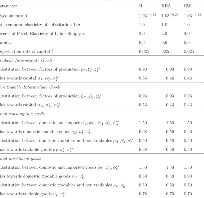
Table 1 contains parameters that regulate preferences and technology. Parameters with “∗” and “∗∗” are related to the REA and the RW, respectively. Throughout we assume perfect symmetry between the REA and the RW, unless differently specified. We assume that discount rates and elasticities of substitution have the same value across the three regions. The discount factorβ is set to 0.9927, so that the steady state real interest rate is equal to 3.0 per cent on an annual basis. The value for the intertemporal elasticity of substitution, 1/σ, is 1. The Frisch labor elasticity is set to 0.5. The depreciation rate of capitalδis set to 0.025. Habit is set to 0.6. In the production functions of tradables and nontradables, the elasticity of substitution be-tween labor and capital is set to 0.93. To match investment-to-GDP ratios, the bias towards capital in the production function of tradables is set to 0.56 in Home and, in the REA and in the RW, to 0.46. The corresponding value in the production function of nontradables is set to 0.53 in Home and 0.43 in the REA and RW. In the final consumption and investment goods the elas-ticity of substitution between domestic and imported tradable is set to 1.5, while the elasticity of substitution between tradables and nontradables to 0.5, as empirical evidence suggests that it is harder to substitute tradables for nontradables than to substitute across tradables. The biases towards the domestically produced good and composite tradable good are chosen to match the Home and REA import-to-GDP ratios. In the consumption bundle the bias towards the domestic tradeable is 0.68 in Home, 0.59 in the REA and 0.90 in the RW. The bias towards the composite tradeable is set to 0.68 in Home, to 0.50 in the REA and the RW. For the investment basket, the bias towards the domestic tradeable is 0.50 in Home, 0.49 in the REA and 0.90 in the RW. The bias towards the composite tradable is 0.78 in Home, 0.70 in the REA and in the RW.
Table 2 reports gross mark-up values. In the Home tradable and nontradable sectors and in the Home labor market the mark-up is set to 1.08, 1.29 and 1.60, respectively (the corresponding elasticities of substitution across varieties are set to 13.32, 4.44 and 2.65). In the REA tradable and nontradable sectors and in the REA labor market the gross mark-ups are respectively set to 1.11, 1.24 and 1.33 (the corresponding elasticities are set to 10.15, 5.19 and 4.00). Similar values are chosen for the corresponding parameters in the RW.
Table 3 contains parameters that regulate the dynamics. Adjustment costs on investment change are set to 6. Nominal wage quadratic adjustment costs are set to 200. In the tradable
sector, we set the nominal adjustment cost parameter to 300 for Home tradable goods sold domestically and in the REA; for Home goods sold in the RW, the corresponding parameter is set to 50. The same parameterization is adopted for the REA, while for the RW we set the adjustment cost on goods exported to Home and the REA to 50. Nominal price adjustment costs are set to 500 in the nontradable sector. The two parameters regulating the adjustment cost paid by the private agents on their net financial position are set to 0.00055 so that they do not greatly affect the model dynamics.
Table 4 reports parametrization of the systematic feedback rules followed by the fiscal and monetary authorities. In the fiscal policy rule (4) we set φ1 = 0.05, φ2 = 1.01 for Home and
φ1=φ2=−1.01 for the REA and the RW. The instrument in the Home fiscal rule depends on
the simulated consolidation. In the case of labor (capital) income tax-based consolidation, the adjusted instrument is the labor (capital) tax rate. When the services reform is implemented in isolation, the adjusted instruments are lump-sum transfers, so that the effects of the structural reform are not affected by fiscal policy (the Ricardian equivalence holds). For REA and RW, it is always lump-sum transfers to adjust. The central bank of the EA targets the contemporaneous EA-wide consumer price inflation (the corresponding parameter is set to 1.7) and the output growth (the parameter is set to 0.1). Interest rate is set in an inertial way and hence its previous-period value enters the rule with a weight equal to 0.87. Same values hold for the corresponding parameters of the Taylor rule in the RW.
Table 5 reports the actual great ratios and tax rates, which are matched in the model steady state under our baseline calibration. We assume a zero steady state net foreign asset position of each region. This implies that for each region - in steady state - the net financial position of the private sector is equal to the public debt. The size of Home and REA GDPs, as a share of world GDP, are set to 3 percent and to 17 percent, respectively.
As for fiscal policy variables, the public consumption-to-GDP ratio is set to 0.20. The tax rate on wage income τℓ is set to 42.6 per cent in Home and to 34.6 in the REA. The tax rate
on physical capital income τk is set to 34.9 in Home and 25.9 in the REA, while the tax rate
on consumptionτc is equal to 16.8 in Home and to 20.3 in the REA. The public debt-to-yearly
are set to values equal to those of corresponding REA variables.
3
Results
In this section we initially describe the simulated scenarios. Subsequently, the long-run (steady-state) and short-run (transition) results are reported. Finally, we conduct some robustness analysis and report the short and medium-run effects of fiscal and competition reforms under al-ternative assumptions about the financing condition of Home households, i.e. when the sovereign spread is temporarily reduced and when the monetary policy rate is held constant.
3.1
Simulated scenarios
The fiscal consolidation scenarios are simulated as follows: we modify the fiscal rule (4) defined on labor (capital) income taxes by assuming that the target value of debt ¯bg becomes a
time-dependent variable. We exogenously specify a path for ¯bg that implies that the Home public
debt-to-(annualized) GDP ratio is decreased by 10 percentage points, from 130 to 120 percent, over a 10-year period.
The competition friendly-reforms in the Home service sector are simulated by gradually re-ducing the sector-specific (gross) mark-up by 5 percentage points, from 1.29 to 1.24 percent over a 10 year-period. When the services reform is implemented in isolation, lump-sum transfers endogenously adjust according to the fiscal rule. As such, the effects of the structural reform are not affected by fiscal policy.
3.2
Long-run effects
We start by illustrating the steady-state effects of labor income based, capital income tax-based consolidation and services reform, implemented in isolation and simultaneously.
3.2.1 Public debt consolidation and tax reduction
Table 6 reports long-run (steady-state) results of permanently reducing the public debt-to-GDP ratio. As interest payments are lower in the final steady-state equilibrium than in the initial one, taxes can be permanently reduced. Column (a) reports the case of reducing the labor income tax rate (other exogenous fiscal items are held at their corresponding initial steady state levels). In correspondence of the new level of debt, the tax rate (not reported) is equal to 42 percentage points, 0.7 percentage points less than its initial value. The increase in labor favours capital productivity. Home (real) output, consumption, investment and employment increase by 0.3, 0.4, 0.2 and 0.4 percent of their corresponding initial steady state levels, respectively.
Column (b) shows the effects of exploiting the reduction in interest payments to decrease the capital income tax rate (from 34.9 to 33.6 percent). GDP, consumption, investment and employment increase by 1.2, 0.6, 2.6 and 0.1 percent, respectively. Investment increases more than in the previous simulation while employment increases less, as the reduction in capital income taxes makes investment cheaper than labor.
In both simulations the excess supply of goods and services induces a depreciation of the Home real exchange rate. The implied effects are two. Domestic tradables become cheaper and the purchasing power of foreign households increases. Both effects favor an increase in Home exports. Home imports increase because of higher domestic demand, notwithstanding the worsening of the Home terms of trade. The effects on the trade variables are larger in the case of capital income tax-based than in that of labor income tax-based consolidation, because the former consolidation strategy has a larger supply-side effect than the latter. The terms of trade deteriorate to absorb the excess supply of Home tradables.
Finally, spillovers to the REA are small, given the relatively small share of Home tradables in foreign aggregate demand.
3.2.2 Increasing competition in the service sector
Column (c) of Table 6 reports the long-run (steady-state) effects of increasing competition in the Home service sector. Firms increase production of services and reduce their prices. This favours the increase in demand of capital and labor for production purposes. The reduction in the price
of services is an incentive for households to increase consumption, given its high services’ content. The increases in GDP, consumption and investment are respectively equal to 1.3, 0.7 and 2.0 percent. Employment also increases, by 0.6 percent. Home exports and imports increase, by 0.6 and 0.2 percent, respectively.
The terms of trade deterioration is lower than the real exchange rate depreciation. The reason is that the increase in the price of domestic tradables partially counterbalances the real exchange rate depreciation. The increase in the price of domestic tradables (expressed in Home consumption units) has two sources. First, tradables and services are complement, hence a higher demand of the latter drives up the demand of the former. Second, higher demand of domestic inputs (labor and capital) drives up marginal costs also in the manufacturing sector, that is not subject to any mark-up-reducing reform.
As in the previous simulation, spillovers to the REA are small (the increase in REA GDP is muted).
3.2.3 Joint implementation of fiscal consolidation and competition reform
Column (d) reports results of implementing (simultaneously) both labor income tax-based con-solidation and the services competition reform. The increase in GDP is larger than in the case of implementing reforms separately, as reported in columns (a) and (c). The reason is that the increase in competition raises Home output and, hence, the labor income tax base. Given the 10 percentage point reduction in public debt-to-GDP ratio, the higher tax base allows to decrease the labor income tax rate by 2.4 percentage points, an amount larger than the one obtained when implementing the fiscal consolidation only, equal to 0.7 percentage points. The additional tax rate reduction further stimulates the economy. Overall, GDP increases by 2.3 percent, consumption by 1.8, investment by 2.7, employment by 1.9.
A similar picture emerges when the competition reform is implemented jointly with the capital income tax-based consolidation (column e). Investment, which is rather elastic in the long run, benefits from the additional reduction in the tax rate, from 34.9 to 31.0 percentage points (to 33.6 percentage points when the fiscal consolidation is implemented in isolation). GDP, consumption, investment and employment increase by 4.9, 2.6, 10.4 and 1.0 percent, respectively.
Overall, results suggest not only that reforms are beneficial, but also that the simultaneous implementation magnifies the macroeconomic impact of the individual reforms. As such, coor-dinating the implementation of fiscal and competition reforms could be a crucial policy measure for maximizing their long-run effectiveness.
3.3
Transition dynamics
In what follows we report the transition dynamics in correspondence of the considered policy measures. The effects of the fiscal consolidation are initially shown. Thereafter, we report those of the competition-enhancing reform in the service sector implemented apart and simultaneously with the fiscal consolidation.
3.3.1 Fiscal consolidation
The top two panels of Figure 1 report the paths of Home labor income tax rate and public debt-to-GDP ratio in the case of labor tax-based consolidation. The fiscal rule (4) commands a gradual increase in the labor tax rate by 2 percentage points in the first six years. As the reduction in the debt-to-GDP ratio progresses, new fiscal room is created to actually reduce the tax rate, because of the lower interest payment. The resulting path of the tax rate is hump-shaped and the consolidation ends up reducing the labor tax rate on a permanent basis below its initial value after 14 years. A similar path characterizes the capital income tax-based consolidation, as reported in the bottom two panels of Figure 1. The tax rate is increased from 34.9 to 37.8 percentage points during the first three years. Thereafter, it gradually decreases and permanently falls below its initial value after 14 years.
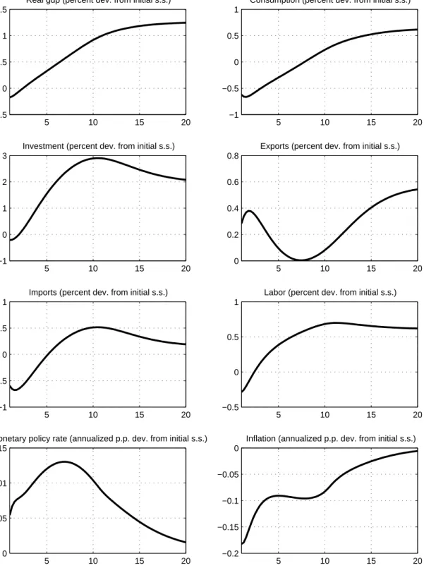
Figure 2 shows the path of the main macroeconomic variables under the assumption of labor tax-based consolidation. The increase in the labor tax has a negative effect on the Home economy. GDP decreases by around 0.7 percent after 10 years (trough level). It persistently stays below the baseline value. Consumption, investment and employment decrease by 0.4, 1.1 and 1.0 percent, respectively. As firms reduce employment, physical capital becomes less productive. Investment becomes less convenient and, hence, decreases. Home exports decrease by 1 percent, because of the loss in price competitiveness. From the 15th year, once the debt-to-GDP ratio has achieved
its new (lower) level, the labor income tax rate starts to be reduced and the main domestic macroeconomic variables increase towards and above their baseline level.
Similar paths characterize the capital income tax-based consolidation scenario, as reported in Figure 3. The short and medium-run effects of the temporary increase in the tax rate on the Home economy are negative. GDP decreases by about 1.5 percent after 8 years. The decrease in investment is large. As for the increase in labor income taxation, there is a temporary negative supply-side effect, that causes a slight increase in inflation and the appreciation of the Home real exchange rate. The implied loss of international price competitiveness reduces Home exports. Imports decrease, mimicking the path of investment. GDP increases above its baseline level after 16 years, in correspondence of the reduction in taxes on capital income.
Overall, tax-based fiscal consolidations inevitably imply short- and medium-run macroeco-nomic costs. The latter have to be compared with the long-run benefits, that are large and permanent. Moreover, short-run costs can be alleviated by other factors, such as the simultane-ous implementation of the reforms in the service sector, as shown in the section after the next one.
3.3.2 Competition reform
Figure 4 shows the macroeconomic effects of the competition reform in the Home service sector. Real GDP slightly decreases in the first year. Two years after the beginning of the reform, GDP is slightly above its baseline level and monotonically increases toward its new long-run level, mainly driven by the increase in the production of services. The initial decrease is associated with households anticipating that services will be cheaper in future than in current periods, when their supply will be large. Given its high services content, households postpone consumption to future periods. Consumption drops in the first two years and then starts to increase but stays below the initial baseline level for around eight years, roughly the amount of time needed to fully implement the reform. Immediately after the beginning of the reform, investment increases, to build a higher stock of capital when production has to be increased (in correspondence of higher competition). The increase in investment drives up demand for domestic tradables. In the medium term exports increase because of the real exchange rate depreciation, associated
with the excess supply of services. Imports initially decrease and thereafter increase mimicking domestic aggregate demand.13
Overall, the service sector reform has medium-run expansionary effects on the Home economy, while their short-run (first-year) effects are slightly negative.
3.3.3 Simultaneous implementation of the fiscal consolidation and competition re-form
The top two panels of Figure 5 report the paths of tax rate and public debt-to-GDP ratio when the labor income tax-based consolidation is jointly implemented with the competition reform. The bottom two panels report the path of tax rate and public debt-to-GDP ratio in the case of joint implementation of capital income tax-based consolidation and competition reform. As in the case of isolated implementations, the public debt is gradually reduced over ten years by alternatively increasing labor income and capital income tax, while the reform in the service sector is implemented over ten years.
Now the tax rates have a less pronounced hump-shaped path than in Figure 1. The relatively quick increase in Home GDP, due to the competition-friendly reform, favours the increase in the labor tax base. Hence, a lower increase in the tax rate is now needed to reduce public debt. The labor and capital income tax rates fall below their corresponding baseline level in a relatively quick way.
Figure 6 reports results when the labor income tax-based consolidation and competition reform are jointly implemented. For comparison, it also contains results of implementing the consolidation in isolation (label “benchmark”, results are the same as in Figure 2). Benefits from the services reform are clear. The increase in competition has a stimulating effect on economic activity. The GDP loss entailed by the fiscal consolidation is mitigated. GDP returns above its baseline level six years after the beginning of the reforms. Thereafter, it monotonically increases, favoured by consumption, investment and gross exports. Labor augments to increase production. Imports increase because of the increase in Home aggregate demand, favoured by the increase in permanent income. All mentioned variables decrease when the fiscal consolidation
13
is implemented in a stand-alone way. Interestingly, expansionary effects are larger than in the case of services reform implemented in isolation (see Figure 4). The additional effect is due to the labor tax rate, that can be reduced below its baseline level after ten years because the services reform favours employment, labor income and, hence, expands the related tax base.
Figure 7 shows results obtained when simultaneously implementing the capital income tax-based consolidation and the reform in the service sector. The message is similar to the one of the previous simulation. There are smaller short-run costs in terms of GDP than in the case of fiscal consolidation. After seven years, GDP is above the baseline and monotonically increases, driven by consumption and investment. This is not the case when it is only the consolidation to be implemented, because the increase in taxes has a negative effect on economic activity. As for labor tax-based consolidation, there is an additional expansionary effect from the simultaneous implementation. The increase in competition allows to reduce the capital income tax rate below its baseline level after ten years, thus benefiting capital accumulation and economic activity (compare Figure 7 with Figure 4).
Overall, we do find that the joint implementation of fiscal consolidation and competition-friendly reforms can benefit the Home economy not only in the long run but also in the short and medium term, by limiting the initial increase in tax rates and hence the implied distortionary effects on economic activity.
4
Conclusions
In the aftermath of the sovereign crisis many European countries have been advised to implement reforms to reduce public debt and structurally improve their economy. In this paper we have evaluated the macroeconomic effects of simultaneously implementing two reforms. One is based on consolidating the public debt. It allows taxes to be reduced in the new long-run equilibrium, once a lower level of public debt has been achieved. The other enhances the degree of competition in the service sector.
According to our results, the simultaneous implementation of both (fiscal and competi-tion) reforms greatly favors the increase of output in the long run. The transition costs of
the fiscal consolidation are substantial; they are reduced if it is implemented jointly with the competition-friendly reform. The reason is the increase in the income tax base, associated with the competition-friendly reform, which allows tax rates to be further reduced in the long run and their increase to be limited in the short run.
This paper does not consider reforms in the labor market and their simultaneous implemen-tation with the policy measures considered in this paper. Moreover, the paper does not consider the possibility that fiscal and service reforms could be simultaneously implemented at EA level when the ZLB is binding. We leave these interesting issues for future research.
References
[1] Benigno, P. (2009). Price Stability with Imperfect Financial Integration.Journal of Money, Credit and Banking, Vol. 41(s1), pages 12–149.
[2] Christoffel, K., G. Coenen and A. Warne (2008). The New Area-Wide Model of the Euro Area: A Micro-Founded Open-Economy Model for Forecasting and Policy Analysis. ECB Working Paper 944, European Central Bank.
[3] Coenen, G., P. McAdam and R. Straub (2008). Tax Reform and Labour-Market Performance in the Euro Area: A Simulation-Based Analysis using the New Area-Wide Model.Journal of Economic Dynamics and Control, vol. 32, pages 2543–2583.
[4] Corsetti, G., K. Kuester, A. Meier and G. J. Mueller (2012). Sovereign Risk, Fiscal Policy, and Macroeconomic Stability. IMF Working Paper 12/33, International Monetary Fund. [5] Corsetti, G., and G. J. Mueller (2006). Twin Deficits: Squaring Theory, Evidence and
Common Sense.Economic Policy,vol. 48, pages 597–638, October.
[6] Draghi, M. (2014). Hearing at the Committee on Economic and Monetary Affairs of the Eu-ropean Parliament Introductory Statement by Mario Draghi, President of the ECB, Brussels, 3 March 2014.
[7] Eggertsson, G., A. Ferrero and A. Raffo (2014). Can Structural Reforms Help Europe?.
Journal of Monetary Economics, vol. 61, pages. 2–22, January.
[8] European Commission (2010). Europe 2020: A European Strategy for Smart, Sustainable and Inclusive Growth. Communication from the Commission to the European Council, March.
[9] European Commission (2012). AMECO Database. [10] Eurostat (2012). Taxation trends in the European Union.
[11] Fern´andez-Villaverde, J., P. Guerr´on-Quintana and J. F. Rubio-Ram´ırez (2012). Supply-Side Policies and the Zero Lower Bound, mimeo.
[12] Fiori, G., G.Nicoletti, S. Scarpetta S. and F. Schiantarelli (2012). Employment Effects of Product and Labour Market Reforms: Are there Synergies?. Economic Journal, 122(558), pages F79-F104, 02.
[13] Forni, L., A. Gerali and M. Pisani (2010a). Macroeconomic Effects Of Greater Competition in the Service Sector: the Case of Italy. Macroeconomic Dynamics, Cambridge University Press, vol. 14(05), pages 677–708, November.
[14] Forni, L., A. Gerali and M. Pisani (2010b). The Macroeconomics of Fiscal Consolidations in Euro area Countries. Journal of Economic Dynamics and Control, Elsevier, vol. 34(9), pages 1791–1812, September.
[15] Gomes, S., P. Jacquinot, M. Mohr and M. Pisani (2013). Structural Reforms and Macroeco-nomic Performance in the Euro Area Countries: A Model-Based Assessment.International Finance, vol. 16(1), pages 23–44, Spring.
[16] Gomes, S., P. Jacquinot and M. Pisani (2010). The EAGLE. A Model for Policy Analysis of Macroeconomic Interdependence in the Euro Area. ECB Working Paper 1195, European Central Bank.
[17] Laubach, T. (2010). Fiscal Policy and Interest Rates: The Role of Sovereign Default Risk. National Bureau of Economic Research International Seminar on Macroeconomics, pages 7–29.
[18] Laxton, D. and P. Pesenti (2003). Monetary Policy Rules for Small, Open, Emerging Economies.Journal of Monetary Economics, vol. 50, pages 1109–1146.
[19] Locarno, A., A. Notarpietro and M. Pisani (2013). Fiscal Multipliers, Monetary Policy and Sovereign Risk: A Structural Model-Based Assessment. Temi di discussione (Working Paper Series) 943, Bank of Italy.
[20] Lusinyan, L. and D. Muir (2013). Assessing the Macroeconomic Impact of Structural Re-forms The Case of Italy. IMF Working Papers 13/22, International Monetary Fund. [21] Pesenti, P. (2008). The Global Economy Model (GEM): Theoretical Framework.IMF Staff
[22] Rotemberg, Julio J. (1982). Monopolistic Price Adjustment and Aggregate Output.Review of Economic Studies,vol. 49, pages 517–31.
Table 1. Parametrization of Home, REA and RW
Parameter H REA RW
Discount rateβ 1.03−0.25 1.03−0.25 1.03−0.25
Intertemporal elasticity of substitution 1/σ 1.0 1.0 1.0 Inverse of Frisch Elasticity of Labor Supplyτ 2.0 2.0 2.0
Habith 0.6 0.6 0.6
Depreciation rate of capitalδ 0.025 0.025 0.025
Tradable Intermediate Goods
Substitution between factors of productionξT, ξT∗, ξ
∗∗
T 0.93 0.93 0.93
Bias towards capitalαT, α∗T, α
∗∗
T 0.56 0.46 0.46
Non tradable Intermediate Goods
Substitution between factors of productionξN, ξN∗, ξ
∗∗
N 0.93 0.93 0.93
Bias towards capitalαN, α∗N, α
∗∗
N 0.53 0.43 0.43
Final consumption goods
Substitution between domestic and imported goodsφA, φ∗A, φ
∗∗
A 1.50 1.50 1.50
Bias towards domestic tradable goodsaH, a∗F, a
∗
G 0.68 0.59 0.90
Substitution between domestic tradables and non tradablesρA, ρ
∗
A, ρ
∗∗
A 0.50 0.50 0.50
Bias towards tradable goodsaT, a∗T, a
∗∗
T 0.68 0.50 0.50
Final investment goods
Substitution between domestic and imported goodsφE, φ∗E, φ
∗∗
E 1.50 1.50 1.50
Bias towards domestic tradable goodsυH, υ∗F 0.50 0.49 0.90
Substitution between domestic tradables and non tradablesρE, ρ∗E 0.50 0.50 0.50
Bias towards tradable goodsυT, υT∗ 0.78 0.70 0.70 Note: H=Home; REA=rest of the euro area; RW= rest of the world.
Table 2. Gross Mark-ups Mark-ups and Elasticities of Substitution Tradables Nontradables Wages
H 1.08 (θT = 13.32) 1.29 (θN = 4.44) 1.60 (ψ= 2.65) REA 1.11 (θ∗ T = 10.15) 1.24 (θ ∗ N = 5.19) 1.33 (ψ ∗ = 4) RW 1.11 (θ∗∗ T = 10.15) 1.24 (θ ∗∗ N = 5.19) 1.33 (ψ ∗∗ = 4)
Note: H=Home; REA=rest of the euro area; RW= rest of the world.
Table 3. Real and Nominal Adjustment Costs Parameter (“∗
” refers to rest of the euro area) H REA RW
Real Adjustment Costs
InvestmentφI,φ∗I, φ
∗∗
I 6.00 6.00 6.00
Households’ financial net positionφb1,φb2 0.00055, 0.00055 - 0.00055, 0.00055
Nominal Adjustment Costs
WagesκW,κ∗W,κ
∗∗
W 200 200 200
Home produced tradablesκH,k∗H k
∗∗
H 300 300 50
REA produced tradablesκH,kH∗ k
∗∗ H 300 300 50 RW produced tradablesκH,kH∗ k ∗∗ H 50 50 300 NontradablesκN,κ∗N,κ ∗∗ N 500 500 500
Note: H=Home; REA=rest of the euro area; RW= rest of the world.
Table 4. Fiscal and Monetary Policy Rules
Parameter H REA EA RW
Fiscal policy rule φ1, φ ∗ 1, φ ∗∗ 1 ±0.05 ±1.01 - ±1.01 φ2, φ ∗ 2, φ ∗∗ 2 ±1.01 ±1.01 - ±1.01
Common monetary policy rule -
-Lagged interest rate at t-1ρR, ρ∗∗R - - 0.87 0.87
InflationρΠ, ρ∗∗Π - - 1.70 1.70
GDP growthρGDP, ρ∗∗GDP - - 0.10 0.10 Note: H=Home; REA=rest of the euro area; EA= euro area; RW= rest of the world.
Table 5. Main macroeconomic variables (ratio to GDP) and tax rates H REA RW Macroeconomic variables Private consumption 61.0 57.1 64.0 Private Investment 18.0 16.0 20.0 Imports 29.0 24.3 4.25
Net Foreign Asset Position 0.0 0.0 0.0 GDP (share of world GDP) 0.03 0.17 0.80
Public expenditures
Public purchases 20.0 20.0 20.0
Interests 4.0 2.0 2.0
Debt (ratio to annual GDP) 130 79 79
Tax Rates
on wage 42.6 34.6 34.6
on rental rate of capital 34.9 25.9 25.9 on price of consumption 16.8 20.3 20.3
Note: H=Home; REA= Rest of the euro area; RW= Rest of the world. Sources:
Table 6. Long-run effects of fiscal and competition reforms. Main macroeconomic variables
(a) (b) (c) (d) (e)
τw τk services services+τw services+τk
Home GDP 0.32 1.17 1.25 2.29 4.92 Consumption 0.35 0.63 0.66 1.76 2.56 Investment 0.24 2.64 1.97 2.74 10.43 Exports 0.35 1.48 0.55 1.65 5.20 Imports 0.11 0.48 0.18 0.54 1.68 Labor 0.40 0.13 0.60 1.88 1.01
Real exch. rate (vis-`a-vis REA) 0.17 0.69 1.57 2.11 3.73 Real exch. rate (vis-`a-vis RW) 0.17 0.68 1.56 2.10 3.71 Terms of trade (vis-`a-vis REA) 0.23 1.00 0.37 1.11 3.50 Terms of trade (vis-`a-vis RW) 0.23 0.98 0.36 1.10 3.43
Rest of euro area
GDP 0.01 0.03 0.01 0.01 0.04
Figure 1. Fiscal consolidation. Tax rates and public debt-to-GDP ratio 5 10 15 20 −1 −0.5 0 0.5 1 1.5 2
Labor income tax rate (percentage point dev. from initial s.s.)
5 10 15 20 108 110 112 114 116 118 120
Public debt−to−annualized GDP ratio (percentage points)
5 10 15 20 −1 −0.5 0 0.5 1 1.5 2 2.5 3
Capital income tax rate (percentage point dev. from initial s.s.)
5 10 15 20 108 110 112 114 116 118 120
Public debt−to−annualized GDP ratio (percentage points)
Figure 2. Labor income tax-based consolidation 5 10 15 20 −0.8 −0.6 −0.4 −0.2 0 0.2
Real gdp (percent dev. from initial s.s.)
5 10 15 20 −0.6 −0.4 −0.2 0 0.2
Consumption (percent dev. from initial s.s.)
5 10 15 20 −1.5 −1 −0.5 0 0.5
Investment (percent dev. from initial s.s.)
5 10 15 20
−1 −0.5 0 0.5
Exports (percent dev. from initial s.s.)
5 10 15 20 −0.2 −0.1 0 0.1 0.2
Imports (percent dev. from initial s.s.)
5 10 15 20 −1.5 −1 −0.5 0 0.5
Labor (percent dev. from initial s.s.)
5 10 15 20 −0.01 −0.005 0 0.005 0.01 0.015
Monetary policy rate (annualized p.p. dev. from initial s.s.)
5 10 15 20 −0.1 −0.05 0 0.05 0.1
Inflation (annualized p.p dev. from initial s.s.)
Figure 3. Capital income tax-based consolidation 5 10 15 20 −2 −1.5 −1 −0.5 0 0.5 1
Real gdp (percent dev. from initial s.s.)
5 10 15 20 −1.5 −1 −0.5 0 0.5
Consumption (percent dev. from initial s.s.)
5 10 15 20
−10 −5 0 5
Investment (percent dev. from initial s.s.)
5 10 15 20 −3 −2 −1 0 1
Exports (percent dev. from initial s.s.)
5 10 15 20 −3 −2 −1 0 1 2
Imports (percent dev. from initial s.s.)
5 10 15 20 −0.8 −0.6 −0.4 −0.2 0 0.2
Labor (percent dev. from initial s.s.)
5 10 15 20 −0.06 −0.04 −0.02 0 0.02 0.04
Monetary policy rate (annualized p.p. dev. from initial s.s.)
5 10 15 20 −0.2 −0.1 0 0.1 0.2
Inflation (annualized p.p. dev. from initial s.s.)
Figure 4. Services reform 5 10 15 20 −0.5 0 0.5 1 1.5
Real gdp (percent dev. from initial s.s.)
5 10 15 20 −1 −0.5 0 0.5 1
Consumption (percent dev. from initial s.s.)
5 10 15 20 −1 0 1 2 3
Investment (percent dev. from initial s.s.)
5 10 15 20 0 0.2 0.4 0.6 0.8
Exports (percent dev. from initial s.s.)
5 10 15 20 −1 −0.5 0 0.5 1
Imports (percent dev. from initial s.s.)
5 10 15 20
−0.5 0 0.5 1
Labor (percent dev. from initial s.s.)
5 10 15 20
0 0.005 0.01 0.015
Monetary policy rate (annualized p.p. dev. from initial s.s.)
5 10 15 20 −0.2 −0.15 −0.1 −0.05 0
Inflation (annualized p.p. dev. from initial s.s.)
Figure 5. Fiscal consolidation and services reform. Tax rates and public debt-to-GDP ratio 2 4 6 8 10 12 14 16 18 20 −3 −2 −1 0 1 2
Labor income tax−based consolidation: labor income tax rate (percentage point dev. from initial s.s.)
2 4 6 8 10 12 14 16 18 20 108 110 112 114 116 118 120
Labor income tax−based consolidation: public debt−to−annualized GDP ratio (percentage points)
2 4 6 8 10 12 14 16 18 20 −4 −2 0 2 4
Capital income tax−based consolidation: capital income tax rate (percentage point dev. from initial s.s.)
2 4 6 8 10 12 14 16 18 20 108 110 112 114 116 118 120
Capital income tax−based consolidation: public debt−to−annualized GDP ratio (percentage points)
Figure 6. Labor income tax-based consolidation and services reform 5 10 15 20 −1 0 1 2 3
Real gdp (percent dev. from initial s.s.) benchmark services 5 10 15 20 −1 −0.5 0 0.5 1 1.5
Consumption (percent dev. from initial s.s.) benchmark services 5 10 15 20 −2 −1 0 1 2 3 4
Investment (percent dev. from initial s.s.) benchmark services 5 10 15 20 −1 −0.5 0 0.5 1 1.5
Exports (percent dev. from initial s.s.) benchmark services 5 10 15 20 −0.5 0 0.5 1
Imports (percent dev. from initial s.s.) benchmark services 5 10 15 20 −2 −1 0 1 2
Labor (percent dev. from initial s.s.) benchmark services 5 10 15 20 −0.01 0 0.01 0.02 0.03
Monetary policy rate (annualized p.p. dev. from initial s.s.) benchmark services 5 10 15 20 −0.15 −0.1 −0.05 0 0.05 0.1
Inflation (annualized p.p. dev. from initial s.s.) benchmark services
Figure 7. Capital income tax-based consolidation and services reform 5 10 15 20 −2 0 2 4 6
Real gdp (percent dev. from initial s.s.) benchmark services 5 10 15 20 −1.5 −1 −0.5 0 0.5 1 1.5
Consumption (percent dev. from initial s.s.) benchmark services 5 10 15 20 −10 −5 0 5 10 15
Investment (percent dev. from initial s.s.) benchmark services 5 10 15 20 −4 −2 0 2 4
Exports (percent dev. from initial s.s.) benchmark services 5 10 15 20 −4 −2 0 2 4
Imports (percent dev. from initial s.s.) benchmark services 5 10 15 20 −1.5 −1 −0.5 0 0.5 1 1.5
Labor (percent dev. from initial s.s.) benchmark services 5 10 15 20 −0.06 −0.04 −0.02 0 0.02 0.04 0.06
Monetary policy rate (annualized p.p. dev. from initial s.s.) benchmark services 5 10 15 20 −0.4 −0.2 0 0.2 0.4
Inflation (annualized p.p. dev. from initial s.s.) benchmark services