Essays on health insurance and the family

(1)

Copyright by

Marcus Owen Dillender 2013

(2)

The Dissertation Committee for Marcus Owen Dillender

certifies that this is the approved version of the following dissertation:

Essays on Health Insurance and the Family

Committee:

Sandra E. Black, Supervisor Jason Abrevaya

Carolyn E. Heinrich Gerald S. Oettinger Daniel S. Hamermesh

(3)

Essays on Health Insurance and the Family

by

Marcus Owen Dillender, B.S.; M.S. Econ.

DISSERTATION

Presented to the Faculty of the Graduate School of The University of Texas at Austin

in Partial Fulfillment of the Requirements

for the Degree of

DOCTOR OF PHILOSOPHY

THE UNIVERSITY OF TEXAS AT AUSTIN May 2013

(4)

(5)

Acknowledgments

I am especially grateful to my advisor, Sandra Black, who provided invaluable support and guidance throughout graduate school. I am also thankful for input and feedback from Jason Abrevaya, Marika Cabral, Daniel Hamermesh, Carolyn Heinrich, Gerald Oettinger, Stephen Trejo, and all of the participants in the University of Texas applied microeconomics seminars.

(6)

Essays on Health Insurance and the Family

Marcus Owen Dillender, Ph.D. The University of Texas at Austin, 2013

Supervisor: Sandra E. Black

The three chapters of this dissertation explore the ties among health insurance, changing cultural institution, and labor economics. The first chapter focuses on the relationship between health insurance and wages by taking advantage of states that extended health insurance dependent coverage to young adults before the Patient Protection and Affordable Care Act. Using American Community Survey and Census data, I find evidence that extending health insurance to young adults raises their wages, both while they are eligible for insurance through their parents’ employers and afterwards. The increases in wages can be explained by increases in human capital and increased flexibility in the labor market that comes from people no longer having to rely on their own employers for health insurance.

The second chapter focuses on understanding the impact of allowing cover-age of spouses through employer-sponsored health insurance. The fact that people choose to enter into marriage makes comparing the differences between married and unmarried couples uninformative. To get around this, I examine how shocks to access to insurance through a spouse’s employer brought on by extensions in legal recogni-tion have influenced health insurance and labor force decisions for same-sex couples. I

(7)

find extending legal recognition to same-sex couples results in female same-sex couples being more likely to have one member not in the labor force.

The third chapter examines what extending legal recognition to same-sex cou-ples has done to marriage rates in the United States using a strategy that compares how marriage rates change after legal recognition in states that alter legal recognition versus states that do not. Despite claims that allowing same-sex couples to marry will reduce the marriage rate for opposite-sex couples, I find no evidence that allowing same-sex couples to marry reduces the opposite-sex marriage rate. The opposite-sex marriage rate does decrease, however, when domestic partnerships are available to opposite-sex couples.

(8)

List of Tables

1.1 Reforms Defining Dependency . . . 8

1.2 College Tuition and Health Insurance Premiums . . . 10

1.3 Descriptive Statistics . . . 14

1.4 The Effect of Extended Health Insurance on Education after Age 25 . 23 1.5 The Effect on Labor Force Participation and College Attendance . . . 24

1.6 The Effect on Labor Force Participation and College Attendance for Married People . . . 25

1.7 The Effect of Extended Health Insurance on Wages after Age 22 . . . 28

1.8 The Effect of Extended Health Insurance on Wages for People Younger than 23 . . . 29

1.9 The Effect of Extended Health Insurance on Labor Force Participation after Age 25 . . . 30

1.10 Predicting the Wage Effects of the Affordable Care Act . . . 34

2.1 States Extending Legal Recognition . . . 45

2.2 Means of Key Variables for Same-Sex Couples in 2006 and 2007 . . . 48

2.3 Effects of Legal Recognition on Identifying Same-Sex Couples . . . . 51

2.4 Means of Key Variables . . . 53

2.5 Labor Force Participation of Female Same-Sex Couples . . . 60

2.6 Labor Force Participation of Male Same-Sex Couples . . . 62

2.7 Effects of Legal Recognition on Health Insurance for Female Same-Sex Couples . . . 65

2.8 Effects of Legal Recognition on Health Insurance for Male Same-Sex Couples . . . 66

2.9 Robustness . . . 68

3.1 Extensions of Legal Recognition by State . . . 80

3.2 Descriptive Statistics . . . 83

(11)

3.4 Time-Varying Effects on Marriage Rates . . . 89

3.5 Effects on Marriage Stocks . . . 91

3.6 Time-Varying Effects on Marriage Stocks . . . 92

3.7 Robustness - Control Group Choice . . . 98

(12)

List of Figures

1.1 Ceofficients from Time Flexible Specification for Men . . . 20

1.2 Ceofficients from Time Flexible Specification for Women . . . 21

1.3 Percent Uninsured by Age, 2008-2010 . . . 33

2.1 Differences in Labor Force Participation . . . 59

2.2 Couples Taking Advantage of Insurance through Spouse’s Employer . 64 3.1 The Trend in National Marriage Rates . . . 79

3.2 Trends in State Overall Marriage Rates . . . 94

(13)

Chapter 1 Do More Health Insurance Options Lead to

Higher Wages: Evidence from States Extending

Dependent Coverage

Labor market and human capital decisions made by young adults can have lasting impacts on their careers. Despite this, little is currently known about how the need for health insurance coverage affects young adults’ labor market decisions. Understanding this is particularly important in light of the fact that extending de-pendent coverage to young adults is a major component of the Affordable Care Act. Economic theory suggests that having access to employer-sponsored health insurance through a source other than one’s own employer could lead to wage increases by re-ducing job-lock, by allowing people to sort into higher paying jobs that do not offer health insurance, and, as this paper finds, by increasing education. Testing this em-pirically is difficult, however, because having an alternate source of health insurance, whether it be through a spouse or a parent, is often the outcome of a joint decision. This paper avoids this endogeneity issue by using plausibly exogenous variation in ac-cess to a parent’s employer-sponsored health insurance plan that is induced by states implementing a minimum age until which employers must provide health insurance to employees’ children.

(14)

in-surance to employees’ children until the age of 26, many states passed reforms that extended dependent coverage to young adults. These reforms gave young adults ac-cess to another source of health insurance apart from school or employment and at a price drastically lower than the private market. Although these reforms increased ac-cess to employer-sponsored health insurance for young adults, research on the reforms suggests they did not have a dramatic effect on overall health insurance coverage lev-els. Both Levine et al. (2011) and Monheit et al. (2011) use health insurance data from the Current Population Survey to study how these reforms affected health in-surance levels. Levine et al. find overall health inin-surance rises by about 3 percentage points for young adults, while Monheit et al. find that the main effect of these reforms was to allow young adults to switch from insurance through their own employers to insurance through their parents’ employers.

Increased flexibility in the labor market and being able to gain employer-sponsored health insurance through a source other than one’s own employer could lead to changes in labor market decisions in a number of ways. First, it could affect education decisions. Attending college at later ages often means people cannot have employer-sponsored health insurance since employers generally allow employees’ chil-dren to stay on their insurance until the age of 22 at the latest in the absence of the reforms. This makes the opportunity cost of attending college after the age of 22 even higher than the forgone wages since employer-sponsored health insurance is typically cheaper and provides more coverage than individual insurance. Additionally, many colleges require students to have health insurance, which essentially raises the price of college for people without easy access to health insurance. Thus, allowing young

(15)

adults to stay on their parents’ health insurance until later ages could lower both the real and opportunity cost of attending college, which could induce marginal people to attend college and then earn higher wages due to their higher human capital.

Second, having a source of health insurance other than through one’s own employer could reduce job-lock, which is the loss of job mobility that arises from the non-portability of employer-sponsored health insurance. As Madrian (1994) argues, with job-lock lessened, people are free to leave their current jobs to find better matches and potentially higher wages. This would be particularly important early in people’s careers before people gain experience in careers that are not their best matches.

Finally, compensating differential theory suggests receiving health insurance through a job should lower wages. This suggests extending dependent coverage to young adults would allow them to earn higher wages by sorting into jobs that do not offer health insurance.

This study contributes to the literature along a number of dimensions. First, the results of this paper help us understand what extending health insurance to young adults does and suggest the Affordable Care Act could increase education and wages for young adults. Second, knowing what extending dependent coverage does to education levels helps us understand people’s education decisions. Increased college attendance at older ages would suggest the U.S. reliance on employer-sponsored health insurance may prevent people from investing in their human capital.

To determine how this new avenue for obtaining health insurance affects young adults’ education and wages, I use data from the Census and the American

(16)

Commu-nity Survey. The estimation strategy compares how education and wages change for eligible young adults after the reforms while accounting for state and national trends. The paper primarily focuses on people older than 22, as younger individuals could generally access parental insurance prior to the change in legislation if they were en-rolled in college. I begin by estimating a time-flexible specification that allows the effects of the reforms to vary by an individual’s age at the time of the reform to show that the reforms begin to affect people 18 or younger at the time of passage, likely because people 18 and younger have not yet made their higher education and labor force decisions and have not left their parents’ health insurance.

I find that wages increase after the age of 22 for those who were 18 or younger when dependent coverage was extended. Wages increase by 2.3 percent for men and 2.9 percent for women when they become eligible for additional health insurance coverage through their parents’ employers. These wage increases largely persist be-yond the time when young adults are eligible for their parents’ health insurance. For men, the persistent changes can be attributed almost entirely to changes in educa-tion, which increases by about 0.18 years on average. However, the education gains for women, which are only about 0.06 years and are statistically insignificant, do not seem to account for much of the wage increase. Labor force participation falls slightly for people in their early twenties as men enroll in college and women take more time before entering the labor force. Once young adults are no longer eligible for insurance through their parents’ employers, labor force participation returns to the pre-reform levels. Scaling the wage estimates to account for the fact that more employers will have to provide coverage under the Affordable Care Act suggests that the Affordable

(17)

Care Act will increase wages by an average of 4.7 to 6.4 percent for people who were 18 or younger when the Affordable Care Act was passed.

The paper unfolds as follows. The next section discusses previous work on health insurance and the labor market. Section 1.2 discusses the extensions in de-pendent coverage and motivates how health insurance could affect education levels. Section 1.3 discusses the costs of extending dependent coverage. Section 1.4 describes the data, econometric issues, and the empirical strategy. Section 1.5 provides the es-timates of the effect of defining dependency status on education levels, education timing, and wages. Section 1.6 provides a discussion of the results, including a possi-ble explanation for why the results might differ for men and women and implications for the Affordable Care Act. Section 1.7 concludes.

1.1 Previous Literature

Employer-sponsored health insurance is cheaper and provides more coverage than individual insurance because of a tax structure that favors employers providing insurance and because risk-pooling is typically easier for employers than for indi-viduals. Furthermore, concerns over adverse selection are a major driving force in the supply-side of the individual market. These factors contribute to the attractive-ness of employer-sponsored health insurance relative to alternative sources of health insurance.1

A major focus of the literature on health insurance and the labor market is 1_{See Currie and Madrian (1999) and Buntin et al. (2004) for discussions of the advantages that} employers have in providing health insurance.

(18)

identifying the effects of an outside source of employer-sponsored health insurance on people’s labor market decisions and outcomes. Much of this work focuses on married women and uses husbands’ insurance coverage to estimate the effect of an outside source of coverage.

Early work identified the effects of an outside source of coverage by treating husbands’ health insurance as exogenous in women’s labor market decisions.2 _There

are two problems with this approach. The first is that the benefits packages of hus-bands are likely correlated with their unobservable ability and, due to assortative mating, with the unobservable ability of wives. Thus, having an outside option in this case is correlated with an individual’s unobserved ability. The second problem, as Currie and Madrian (1999) point out, is that labor force decisions for married men and women may be the outcome of a joint decision, meaning treating one person’s health insurance as exogenous may yield inconsistent estimates.

Olson (2002) and Kapinos (2009) deal with assortative mating by instrument-ing for a husband’s insurance coverage usinstrument-ing various characteristics of the husband’s job. They find an outside source of insurance coverage raises wages and lowers labor force participation. Although both Olson and Kapinos carefully consider assortative mating, they still make the problematic assumption that couples do not make joint decisions.

This study addresses two key limitations with this literature. The first is one of internal validity in that this paper focuses on an environment in which people 2_{See Buchmueller and Valletta (1999), Holtz-Eakin, et al. (1996), and Lombard (2001) for} ex-amples.

(19)

making joint decisions is less of a concern since children cannot supply their parents with health insurance. This paper also uses plausibly exogenous variation in the ability to access the outside coverage, meaning the results hold even though parents and children have correlated unobservable traits.

This paper also contributes to the literature by focusing specifically on young adults. Since young adults are at the beginning of their careers, facilitating the job match process may matter more than for other ages and young people may be more likely to invest in their human capital. This is important to know as the United States continues its process of healthcare reform. Young adults being able to use their expanded health insurance options to earn higher lifetime wages indicates the advantages of extending dependent coverage go beyond shifting insurance rates.

1.2 Institutional Details

1.2.1 Defining Dependency Status

Young adults are significantly less likely to be insured than older adults. For the years 2008-2010, 31.1 percent of men and 23.6 percent of women ages 18 to 24 were uninsured, while 18.6 percent of men and 14.7 percent of women ages 25 to 64 were uninsured. This may be due to a number of factors, including the inability to afford health insurance or the decision that it is unnecessary given their age and relative health.3

To address the insurance disparities, many states began requiring employers 3_{See Monheit et al. (2011), Nicholson et al. (2009), and Levy (2007) for more thorough discussions} of uninsured rates among young adults and their implications.

(20)

to allow employees’ children to remain on their parents’ health insurance plans until later ages. Between 1995 and 2010, thirty-five states formally defined dependency status. Table 1.1 lists the reforms by state. When dependency status is defined, the maximum ages span from 22 to 30.4

Table 1.1: Reforms Defining Dependency

State Age Effective State Age Effective

State Limit Year State Limit Year

Colorado 25 2006 New Hampshire 26 2007 Connecticut 26 2009 New Jersey 30 2006

Delaware 24 2007 New Mexico 25 2003

Florida 25 2007 New York 29 2009

Georgia 25 2006 North Dakota 26 1995

Idaho 25 2007 Ohio 28 2010

Illinois 26 2004 Pennsylvania 30 2010

Indiana 24 2007 Rhode Island 25 2007

Iowa 24 2008 South Carolina 22 2008

Kentucky 25 2008 South Dakota 24 2007

Louisiana 24 2009 Tennessee 24 2008

Maine 25 2007 Texas 25 2004

Maryland 24 2008 Utah 26 1995

Massachusetts 26 2007 Virginia 25 2007

Minnesota 25 2008 Washington 25 2006

Montana 25 2008 West Virginia 25 2007

Nebraska 30 2010 Wisconsin 27 2010

Nevada 24 1995

Sources: Data on the reforms come from Monheit et al. (2011) as well as data from the National Conference of State Legislatures.

Before the changes in the reforms, the age at which young adults were no longer 4_{Data on the reforms come from Monheit et al. (2011) as well as data from the National} Con-ference of State Legislatures. In most cases, these two sources have identical information on the reforms. When they conflict, I contacted the state insurance department directly or referred to the state legal code.

(21)

eligible for health insurance through their parents’ employers typically depended on specific employers’ policies. Employers traditionally provided coverage for dependents through age 22 if the dependent is enrolled in college and through age 18 otherwise (Government Accountability Office (2008)). States typically require that young adults are unmarried to be eligible for their parents’ health insurance since married people can often access insurance through a spouse’s employer.5 6

Self-insured employers are covered by federal law due to the 1974 Employee Retirement Income Security Act; therefore, they have no obligation to extend de-pendent coverage. This is a key difference between these state-level reforms and the Affordable Care Act. In Section 1.6, I compute what the effects of the reforms may be when self-insured employers have to comply as well.

1.2.2 Schooling and Health Insurance

In addition to having employer-sponsored health insurance, young people can often gain coverage from the individual market or through a school insurance plan if they are in college. According to the Government Accountability Office, about half of 5_{Extending health insurance for dependents has the potential to affect marriage decisions if part} of the reason that people marry in the absence of the reforms is so they can have health insurance through a spouse’s employer. This could affect wages because men tend to experience a marriage premium, while some evidence suggests women experience a marriage penalty. See Ahituv and Lerman (2007) for a thorough summary of this literature as well as some new results. In results not shown, I find no evidence that extending dependent coverage affects marriage decisions.

6_{A few states have other requirements, such as school attendance and residence with parents.} Because this paper focuses on the effects for people at older ages, only early-adopting states provide useful variation. Most of these have no financial dependency or college attendance requirement, meaning these results can generally be thought of as applying to states without a financial depen-dency requirement. All results still hold if all states with stricter requirements are dropped from the sample.

(22)

colleges offer student health insurance plans. Despite these other options, a majority of college students have health insurance through their parents’ employers, likely because of the cost advantage of this source of coverage. In 2008, the Government Accountability Office found about 67 percent of students aged 18 through 23 were covered through their parents’ employer-sponsored plans, while 80 percent of college students had health insurance from any source.

Much research shows the price advantage of employer-sponsored health insur-ance induces people to participate in the labor force. With young adults, the price advantage could cause marginal people to work instead of attend school. This applies at both the college and high school levels. Thus, once young adults can stay on their parents’ health insurance until later ages, the opportunity cost of being in school falls.

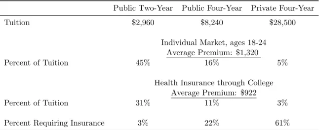
Table 1.2: College Tuition and Health Insurance Premiums

Public Two-Year Public Four-Year Private Four-Year

Tuition $2,960 $8,240 $28,500

Individual Market, ages 18-24 Average Premium: $1,320

Percent of Tuition 45% 16% 5%

Health Insurance through College Average Premium: $922

Percent of Tuition 31% 11% 3%

Percent Requiring Insurance 3% 22% 61%

Notes: The average health insurance premium in the individual market is as of February 2011. The average deductible purchased is around $3,000. The tuition and the premiums for health insurance through college are for the 2011-12 school year. Sources: College Board, Government Accountability Office, eHealthInsurance report.

(23)

Another mechanism for health insurance being related to college attendance is that, as of 2008, 30 percent of colleges required students to have health insurance (Government Accountability Office 2008). This effectively increases the cost of college for anyone without outside coverage, suggesting that extending dependent coverage may effectively reduce the cost of college for people at older ages since people older than 22 cannot be on their parents’ plans before the reforms. Table 1.2 shows average tuition cost by type of college as well as the average price of individual plans and student health insurance plans. Two-year schools requiring insurance would impose the highest effective cost increase as a percent of tuition, while private colleges are more likely to require insurance coverage.

1.3 The Cost of Extending Dependent Coverage

Who pays the costs for this increased access to health insurance is unclear. One possibility is that employers do not pass on the costs to families taking advantage of extended dependent coverage. Instead, employers could allow those employees to pay the same amount for health insurance and receive the same wages. This might result in lower profits for the firm or slightly lower wages for all employees. In this case, this health insurance is very cheap for young people relative to other options.

Previous work on mandated coverage, however, suggests employers are suc-cessful in passing costs onto the affected population in the form of lower wages. This would mean that parents with adult children would have lower wages after dependent

(24)

coverage is extended.7 _{Alternatively, employers could require parents to pay a higher}

premium for each additional child on the insurance plan. In both of these cases, the parents would bear the costs. Parents may then require their children to compensate them for the health insurance, meaning extended dependent coverage may not be free for young adults.8

It is important to note that extending dependent coverage still has the po-tential to affect young adults’ labor market decisions even if the young adults bear the full cost of the coverage. This is because extending dependent coverage provides young adults with a source of low cost and high benefit coverage without being in the labor force themselves.

This paper estimates the reduced form effect of extending dependent coverage after any cost shifting by employers and parents. Although knowing the exact price changes young adults face would be useful, this is the ideal setting for studying the likely effects of the Affordable Care Act because any cost shifting by firms and parents would presumably happen in similar ways when dependent coverage is available for more young adults under the Affordable Care Act.

7_{See Gruber (1994) for an example of research finding firms pass costs of mandated coverage to} employers.

8_{Identifying the effects of extended health insurance on parents’ wages is difficult because most} eligible children no longer live at home. Using data from the Current Population Survey, I find no evidence that wages or insurance coverage fall for a sample of older adults.

(25)

1.4 Data and the Empirical Strategy

1.4.1 Data and Descriptive Statistics

The data on individuals come from the 1990 and 2000 Censuses as well as the 2001-2010 American Community Surveys. Until 2000, the Census asked individuals detailed questions about their demographics and labor market outcomes. Beginning in 2000, the Census Bureau began asking these questions in the American Community Survey instead of the Census. The American Community Survey has smaller sample sizes than the Census but provides yearly data. The advantages of these data sets are that they are large and representative and provide precise estimates of the reduced form effect of extending dependent coverage for young adults.

The estimation uses data on wages, education, and demographic character-istics. I compute the real hourly wage in 2005 dollars by dividing the yearly wage income in 2005 dollars by the product of number of weeks worked and usual hours worked in a week.9 _{I then take the log of real wages to use as my dependent variable}

when I study wages.

When the dependent variable is completed education, the sample will include people over the age of 25 because, as Card (1999) argues, most people reach their ultimate educational attainment by their mid-twenties. Whenever the dependent variable is wages, I consider people over the age of 22 and those between the ages of 18 and 23 separately because I want to compare people at similar points in their careers 9_{The American Community Survey reports number of weeks worked in an interval, so the hourly} real wage is obtained by taking the real wage income in 2005 dollars divided by the middle number of weeks in the interval multiplied by the usual hours worked in a week.

(26)

Table 1.3: Descriptive Statistics Men

Ages 19 to 22 Ages 23 to 35

Standard Standard

Mean deviation Mean deviation

Education 12.15 1.48 13.15 2.52 College 0.03 0.17 0.25 0.44 Some College 0.38 0.49 0.50 0.50 High School 0.84 0.36 0.87 0.33 In College 0.41 0.49 0.12 0.32 Age 20.44 1.12 29.08 3.74 Hourly Wage 11.05 101.09 17.79 53.92 Log Hourly Wage 2.13 0.68 2.67 0.68

White 0.74 0.44 0.76 0.43 Black 0.12 0.32 0.10 0.30 Hispanic 0.05 0.22 0.05 0.22 Working 0.63 0.48 0.83 0.38 n 1,266,414 3,943,126 Women Ages 19 to 22 Ages 23 to 35 Standard Standard

Mean deviation Mean deviation

Education 12.45 1.46 13.48 2.48 College 0.05 0.22 0.30 0.46 Some College 0.48 0.50 0.58 0.49 High School 0.89 0.31 0.90 0.30 In College 0.51 0.50 0.14 0.35 Age 20.45 1.12 29.10 3.73 Hourly Wage 10.16 21.41 16.18 32.45 Log Hourly Wage 2.04 0.68 2.52 0.69

White 0.74 0.44 0.75 0.43

Black 0.13 0.33 0.12 0.32

Hispanic 0.05 0.22 0.05 0.22

Working 0.60 0.49 0.69 0.46

(27)

and because we know people over the age of 22 cannot typically be on their parents’ insurance plans in the absence of the reforms, while people under 22 sometimes can be. In order for people at similar ages to be compared to each other, I restrict the data to include only people 35 and younger.10 _{The 1990 Census does not ask about}

current school attendance so the results for education timing draw on only the 2000 Census and the American Community Surveys.

The descriptive statistics are shown in Table 1.3. While the means of the race and age variables are similar for both age groups for men and women, women tend to have more education at all levels, while men tend to have higher wages.

1.4.2 Empirical Strategy

The empirical strategy takes advantage of the facts that the reforms were passed at different times and only affect certain people within states that passed the reforms. The first set of results considers the effects of these reforms on completed education. The empirical strategy can be summarized by the following equation:

yist=φst +Xistα+ageistβ1t+ageistβ2s+β3prevtreatedist+ist, (1.1)

where i indexes individual, t year, s state, y represents completed education, φ is a vector of state-year fixed effects, X is a vector of additional controls that includes race, and age is a vector of age indicators equal to one for the individual’s age and zero for all other ages. The variable prevtreated, defined formally below, refers to 10_{Restricting the sample to young people is also important if wages for older people fall because} older people are now relatively more expensive to employ.

(28)

whether or not the individual was at an age such that he would have been affected by the reform during his early twenties. It will vary for different ages within a state after the reform is passed; thus,β3will be the triple-difference estimator of the effect of the

reform. Identification comes from comparing how completed education changes for affected ages after the reforms relative to slightly older ages in states that implement the reform relative to those that do not.

Equation (1.1) contains fixed effects for each state and year combination as well as different base levels for each age and state and age and year combinations. Using variation across cohorts within a state and year means that even if states with certain unobservable characteristics implement the reform, consistent estimation is still achieved so long as these characteristics are fixed over time or any changes affect all young adults. The identification strategy is valid as long as characteristics do not change in ways that affect wages and education for people young enough to be affected by the reforms but not people a few years older.

The goal is to defineprevtreatedto be a one if the individual would have gone through his or her early twenties affected by extended dependent coverage and zero otherwise. However, we need to be careful in thinking about who would be affected by these reforms. For instance, if people are 25 years old when legislation is passed that extends health insurance to people up to age 26, they technically have a new health insurance option available to them, but we would expect little effect on these people’s education and wages because they have already left their parents’ health insurance and made their education and labor force decisions.

(29)

how the effects vary by people’s age at the time of reform, I estimate

yist =φst+Xistα+ageistβ1t+ageistβ2s+

X

j∈J

β3jagerjist+ist, (1.2)

whereagerj _{is a one if the individual was age} _j _{when the reform was passed and zero}

otherwise and J is the set of all ages between 10 and 36 except age 27, meaning all of the coefficients are relative to the effects on people age 27 when the reforms were passed. Age 27 was chosen as the reference age because most of the reforms have an age minimum under 27, meaning there should be no effect for people who were 27 when the reform was passed. Note that ager = age−(year −yearr), where yearr

is the year the reform was passed. We can interpret β3j as being how the reform

affects people who were age j at the time of the reform versus people who were age 27 at the time of the reform. Although theβ3 coefficients are too noisy to distinguish

among, I graph the coefficients in the next section so we can see how the effects of these reforms vary with age at the time of passage.

Estimating Equation (1.2) will indicate the reforms primarily affect education and wages for people who were 18 or younger at the time of the reform. This is likely because people who were 18 or younger at the time of the reform are likely to have not left their parents’ insurance plans or made college or career decisions yet. Because of the results from estimating Equation (1.2), prevtreatedin Equation (1.1) will be a one if the individual was 18 or younger at the time of the reform but is older than the minimum age set by the reform at the time of the observation, or

prevtreated = 1(ager ≤ 18)∗1(age > agemin), where agemin is the age minimum for dependent coverage set by the state. This means people at certain ages will have

(30)

been affected by the reforms while others will not have been.

The results also consider education timing. With education timing, we are no longer interested in whether or not a person was previously treated. Instead, the focus is on people who currently have access to their parents’ health insurance. Because people typically have access to their parents’ health insurance if they are in college if they are younger than 23, I will distinguish between the effects on people during traditional college ages, or people between the ages of 18 and 23, and the effects on people outside of traditional college ages, or people older than 22. To do this, I include everyone between 18 and 27 in the sample and estimate

yist =φst+Xistα+ageistβ1t+ageistβ2s+β3currtreatedist∗youngist

+β4currtreatedist∗olderist+ist, (1.3)

currtreatedis a one for people who were 18 or younger at the time of the reform and are currently eligible for insurance through their parents’ employers, orcurrtreated= 1(ager ≤ 18)∗1(age ≤agemins), young is an indicator variable equal to one if the

individual is older than 18 and younger than 23, and older is an indicator variable equal to one if the individual is older than 22. The coefficient β3 is the effect of the

reform on people during traditional college ages, while the coefficient β4 is the effect

of the reform on people who are older than traditional college ages. We would expect

β3 to be close to zero and β4 to be positive if extending dependent coverage affects

completed education by allowing people to go back to school at later ages.

Equation (1.1) is sufficient for estimating the effect on education because the sample will include only people over the age of 25 and because education is

(31)

nonde-creasing over time, meaning any education increases will persist. When the depen-dent variable is wages, however, distinguishing between the effects for people who are currently eligible for extended dependent coverage and those who were previously eligible but no longer are is important. Thus, when wages are on the left-hand side, the estimating equation becomes

yist=φst+Xistα+ageistβ1t+ageistβ2s+β3currtreatedist

+β4prevtreatedist+ist. (1.4)

In this equation,β3 is the effect of the reform on people who are currently eligible for

extended dependent coverage, while β4 is the persistent effect after people no longer

have access to their parents’ insurance.

1.5 The Effect on Young Adults of Extending Dependent

Coverage

1.5.1 Education

To verify that prevtreated in Equation (1.1) is defined correctly, I begin by estimating Equation (1.2) with completed education as the dependent variable. The sample includes everyone over the age of 25. Although the results are too noisy to find significant effects for any given year, I graph the β3 coefficients for men and women

(32)

Figure 1.1: This figure shows the coefficients on age at the time of reform from estimating Equation (1.2) for men. The dependent variable is completed education.

(33)

Figure 1.2: This figure shows the coefficients on age at the time of reform from estimating Equation (1.2) for women. The dependent variable is completed education.

From Figure 1, we can see that the reforms had no effect on education for men at older ages when the reforms were passed. Even for people who could technically go back to their parents’ insurance, there is little evidence of an effect of the reforms on people’s completed education. However, men who were 18 or younger at the time of the reform experience increased education by the time they are older than 25. This suggests the reforms only have effects on education for people who had not yet left their parents’ insurance and have not yet made college and labor market decisions at the time of the reform. Figure 2 shows a similar pattern for women although

(34)

there appears that there might be a small effect on women at slightly older ages. In results not shown, I verify that all of the results hold if a separate variable is included that captures all of the variation coming from people who were ever eligible for insurance through their parents’ employers, even if they were the same age as the age requirement when the reforms were passed.

Table 1.4 displays the average effects obtained from estimating Equation (1.1) for men and women with the treated variable equal to a one if the individual is 18 or younger when the reform is passed. In column 1, we see that men who were 18 or younger at the time of the reform have an extra 0.183 years of education on average by the time they are older than 25. In column 2, the dependent variable is a one if people have completed college. The coefficient of 0.025 suggests men are 2.5 percentage points more likely to have completed college by the time they are 26 as a result of dependent coverage being extended. The estimate in column 3 suggests men are 2.6 percentage points more likely have attended some college. In column 4, we can see that there is a smaller but significant effect on the likelihood of completing high school of 1.7 percentage points.

For women the coefficients are generally much smaller and do not show any statistically significant effect except on completing high school. The coefficient in column 1 is 0.055. The coefficients on completing college and completing some college are insignificant and close to zero. The coefficient on completing high school suggests about a one percentage point increase in the number of women graduating from high school.

(35)

Table 1.4: The Effect of Extended Health Insurance on Education after Age 25

Men

Years of Completed Completed Completed education college some college high school Previously Treated 0.183*** 0.025** 0.026*** 0.017***

(0.061) (0.009) (0.006) (0.006) Women

Previously Treated 0.055 -0.006 0.004 0.012*

(0.062) (0.008) (0.018) (0.007) Notes: *, **, and *** indicate significance at 10%, 5%, and 1% respec-tively. Standard errors are clustered by state and are shown in parentheses. All specifications include state-year fixed effects, age indicators interacted with state indicators, age indicators interacted with year indicators, and race controls. There are 3,059,508 observations for men and 3,076,784 ob-servations for women.

1.5.2 Education Timing

The results suggest extending health insurance to young adults increases ed-ucation, especially for men. As noted earlier, employers typically allow employees’ children to stay on their health insurance until they are age 22 if they are in col-lege, meaning we would expect extending dependent coverage to affect people at later ages and not at traditional college ages. I now provide evidence that the people who experienced increased education did so after typical college ages.

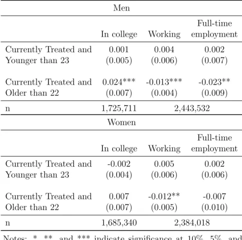
Column 1 of Table 1.5 contains estimates of Equation (1.3) with the dependent variable equal to one if the individual is currently attending college and zero otherwise. The sample includes everyone between the ages of 18 and 27.

(36)

Table 1.5: The Effect on Labor Force Participation and College Attendance

Men

Full-time In college Working employment Currently Treated and 0.001 0.004 0.002 Younger than 23 (0.005) (0.006) (0.007) Currently Treated and 0.024*** -0.013*** -0.023**

Older than 22 (0.007) (0.004) (0.009)

n 1,725,711 2,443,532

Women

Full-time In college Working employment Currently Treated and -0.002 0.005 0.002 Younger than 23 (0.004) (0.006) (0.006) Currently Treated and 0.007 -0.012** -0.007

Older than 22 (0.007) (0.005) (0.010)

n 1,685,340 2,384,018

Notes: *, **, and *** indicate significance at 10%, 5%, and 1% respectively. Standard errors are clustered by state and are shown in parentheses. All specifications include state-year fixed effects, age indicators interacted with state indicators, age indicators interacted with year indicators, and race controls.

(37)

Table 1.6: The Effect on Labor Force Participation and College Attendance for Married People

Men

Full-time In college Working employment Currently Treated and 0.001 0.012 0.010 Younger than 23 (0.021) (0.011) (0.008) Currently Treated and 0.001 0.008 0.003 Older than 22 (0.013) (0.014) (0.010)

n 333,036 513,451

Women

Full-time In college Working employment Currently Treated and 0.004 -0.001 0.006 Younger than 23 (0.020) (0.014) (0.009) Currently Treated and -0.021 -0.005 0.010 Older than 22 (0.016) (0.009) (0.007)

(38)

The results show that there is no evidence of an effect on college attendance for people 22 and younger. For both men and women, the coefficients are insignificant and close to zero for people younger than 23. Men who were 18 or younger at the time of the reform are 2.4 percentage points more likely to be in college when they are older than 22. This suggests, as expected, extended dependent coverage affects only individuals who were not already covered under their parents’ plans. About 15 percent of men were still in college between the ages of 22 and 26, indicating extending dependent coverage increases the number of people still in college between these ages by about 16 percent.

In columns 2 and 3 of Table 1.5, I examine the probability that an individual is working and the probability that the individual has full-time employment. The coefficients for people older than 22 and still eligible for health insurance are negative and significant for both men and women. People are slightly more than one per-centage point less likely to be working after the age of 22 while they can still access insurance through their parents’ employers. The decrease in full-time employment is even greater for men with a coefficient of -0.023. This suggests men are using the increased access to health insurance to leave the labor force and go back to school. Women are not significantly more likely to be in college, but they may still experience wage increases if they spend more time searching for a job that is a better match and will give them higher wages.

For people to be eligible for insurance through their parents’ employers, they have to be unmarried in most states. This means these reforms should have no effect on married people. As a robustness test, I restrict the sample to include only married

(39)

people and verify that nothing happens to the education and labor force participation decisions of married people after dependent coverage is extended. Table 1.6 reports the results. All of the coefficients are insignificantly different from zero. The only point estimate that appears that it might be different than zero–the coefficient on currently treated and older than 22 for women–is the wrong sign.

1.5.3 Wages

To examine wages, I first focus on everyone over the age of 22 and younger than 36. Column 1 of Table 1.7 contains the results from estimating Equation (1.4). The coefficient on Currently Treated is the impact on wages for people who were 18 or younger at the time of the reform and are currently eligible for insurance through their parents’ employers. The estimates suggest wages rise by 2.3 percent for men and by 2.9 percent for women while they are eligible for extended dependent coverage.

The coefficients on Previously Treated test whether or not these effects persist even after young adults are no longer eligible for insurance through their parents’ employers. The coefficients of 0.021 and 0.026 for men and women, respectively, indicate that these effects largely persist for both men and women.

The first specification did not control for education because, as was shown earlier, education is endogenous. Column 2 replicates the regressions from column 1 except that it controls for education. The coefficients for people currently treated in column 2 are smaller but still positive and significant for both men and women. For previously treated people, however, the effect for men is almost zero after control-ling for education, while the effect for women changes very little. This suggests the

(40)

Table 1.7: The Effect of Extended Health Insurance on Wages after Age 22

Men Currently Treated 0.023** 0.018** (0.009) (0.008) Previously Treated 0.021*** 0.006 (0.005) (0.004) Education 0.079*** (0.002) Women Currently Treated 0.029** 0.022* (0.013) (0.012) Previously Treated 0.026*** 0.025*** (0.008) (0.004) Education 0.101*** (0.001) Notes: *, **, and *** indicate significance at 10%, 5%, and 1% respectively. Stan-dard errors are clustered by state and are shown in parentheses. All specifications in-clude state-year fixed effects, age indicators interacted with state indicators, age indi-cators interacted with year indiindi-cators, and race controls. There are 3,443,327 observa-tions for men and 3,006,756 observaobserva-tions for women.

(41)

increases in education for men explain most of the persistent wage increases, while education changes can account for little of the wage increases for women.

Table 1.8: The Effect of Extended Health Insurance on Wages for People Younger than 23 Men Currently Treated -0.001 -0.001 (0.009) (0.009) Education 0.031*** (0.002) Women Currently Treated -0.007 -0.007 (0.005) (0.005) Education 0.044*** (0.002) Notes: *, **, and *** indicate signifi-cance at 10%, 5%, and 1% respectively. Standard errors are clustered by state and are shown in parentheses. All spec-ifications include state-year fixed effects, age indicators interacted with state in-dicators, age indicators interacted with year indicators, and race controls. There are 1,028,256 observations for men and 955,075 observations for women.

In Table 1.8, I present the equivalent estimates of Currently Treated for people younger than 23 and find no effects for people at these ages. This could be because the effects of having more insurance options may take time to manifest themselves or because people at these ages often have coverage in the absence of the reforms.

(42)

Table 1.9: The Effect of Extended Health In-surance on Labor Force Participation after Age 25 Men Full-time Working employment Previously Treated 0.002 0.001 (0.008) (0.001) Women Full-time Working employment Previously Treated 0.006 0.007 (0.005) (0.007) Notes: *, **, and *** indicate significance at 10%, 5%, and 1% respectively. Standard er-rors are clustered by state and are shown in parentheses. All specifications include state-year fixed effects, age indicators interacted with state indicators, age indicators interacted with year indicators, and race controls. There are 3,059,508 observations for men and 3,076,784 observations for women.

(43)

All of these estimates are conditional on people being in the labor force. As was shown above, people are less likely to be in the labor force when they are eligible for health insurance through their parents’ employers. One possibility is that people exit the labor force because they would have received a low wage, which would cause the average wage of working people to rise even if access to health insurance has no causal impact on wages. Alternatively, people going back to school may be higher ability on average, meaning the estimates may be biased downwards. I next estimate Equation (1.1) with indicators for working and full-time employment as the dependent variables to see if affected people return to the labor force after they are no longer eligible for health insurance through their parents’ employers. The coefficients on having been previously treated are shown in Table 1.9. For men and women, the coefficients are close to zero and insignificant. Although people are less likely to work while they have access to their parents’ health insurance, they return to the labor force after eligibility at similar levels as people in the state before the reforms. These wage increases persist even after eligibility, though, suggesting selection is not driving the wage increases.

1.6 Discussion

1.6.1 Explaining the Heterogeneous Effects for Men and Women

Both young men and women experience wage increases as a result of having dependent coverage extended to them; however, the underlying mechanisms appear to be different. Education seems to explain part of the wage increases for men but not for women.

(44)

One plausible explanation is that women have a higher demand for health insurance. Part of this is due to differences in risk aversion between men and women. Numerous studies have documented that women tend to be more risk averse than men.11 _{Another reason women would have a greater demand for health insurance is}

that they are more likely to have higher costs at this age because they may become pregnant.

This suggests that men would be less likely to have health insurance than women. Using data from the American Community Survey, I graph the rates of uninsurance by age for men and women in Figure 1.3. Men are significantly more likely to be uninsured at all ages. At age 23, where uninsured rates peak for both men and women, women are about 10 percentage points more likely to have health insurance.

11_{For examples, see Jianakoplos and Bernasek (1998), Barber and Odean (2001), Hartog et al.} (2002), Agnew et al. (2008), and Borghans et al. (2009).

(45)

Figure 1.3: Percent Uninsured by Age, 2008-2010

Women’s increased desire for health insurance could lead to the wage penalties associated with employer-sponsored health insurance. This suggests that extending health insurance to young women would enable them to move to higher paying jobs that do not offer health insurance. Since they already desire health insurance, requir-ing them to have health insurance before enterrequir-ing into school does not increase the price of schooling. Men not desiring health insurance as much means job-lock should not be a major driving force in their wages in the absence of extended dependent coverage because being uninsured is not as large a concern; however, since they are less likely to have health insurance, they are more likely to have a higher effective cost of attending college since attending college will require that they purchase health

(46)

insurance. Providing young men with more options for health insurance lowers this cost.

1.6.2 Implications for the Affordable Care Act

The results show that wages increase for young adults while they are eligible for dependent coverage and that these wage increases persist even after young adults are no longer eligible for insurance through their parents’ employers. I now calculate what the estimates in this paper suggest will be the effect of the Affordable Care Act.

Table 1.10: Predicting the Wage Effects of the Af-fordable Care Act

Effects on Currently Treated Effect on Predicted Effect of Log Wages the Affordable Care Act

Men 0.023 0.051

(0.009)

Women 0.029 0.064

(0.013)

Persistent Effects

Effect on Predicted Effect of Log Wages the Affordable Care Act

Men 0.021 0.047

(0.005)

Women 0.026 0.058

(0.008)

The Affordable Care Act requires employers to allow employees’ children to stay on their insurance until age 26. There are two main differences between this provision of the Affordable Care Act and the state-level reforms. The first is that

(47)

everyone will be eligible to be on their parents’ health insurance plan under the Affordable Care Act. Almost all of the reforms discussed in this paper require that people be unmarried. We would expect the Affordable Care Act to have smaller effects for married people since many married people have access to health insurance through their spouse’s employer, meaning they already have access to employer-sponsored health insurance through a source other than their own employer.12 I compute the predicted effect of the Affordable Care Act assuming no effect on married couples, meaning the results here are a lower bound on the impact of the Affordable Care Act. The second difference between the state-level reforms and the Affordable Care Act is that self-insured employers will also have to comply with the Affordable Care Act. This will allow more people to receive health insurance through their parents’ employers and will thus result in a higher average wage increase. Recent estimates suggest that 55 percent of people with employer-sponsored health insurance have it through self-insuring employers (Employee Benefit Research Institute (2009)). This number implies the estimates should be scaled up by a factor of 2.2 since more people will have access to dependent coverage.13

Table 1.10 displays the predictions for wages. The estimates presented earlier suggest that men experience wage increases of 2.3 percent and women experience wage 12_{Data from the CPS indicates about 28 percent of people age 23 to 26 were married in 2010 and} that about half of young married couples take advantage of the ability to gain insurance through a spouse’s employer.

13_{Another difference between these state-level reforms and the Affordable Care Act is that the} Affordable Care Act has an age minimum of 26, while the age minimums for the state reforms vary. Allowing the estimates of the state-level reforms to vary by the number of years of additional coverage produces very similar predictions for the Affordable Care Act.

(48)

increases of 2.9 percent while they have access to their parents’ health insurance. When self-insured employers have to comply, we might expect effect sizes of 5.1 percent for men and 6.4 percent for women, which would be over a $9,000,000 increase in total earnings in 2010 dollars for people ages 23 to 26. The estimates of the persistent effects from earlier suggest the affected cohort of men has 2.1 percent higher wages, while the affected cohort of women has 2.6 percent higher wages. Scaling the estimates for the Affordable Care Act suggests wages will increase by 4.7 percent for men 5.8 percent for women.14

1.7 Conclusion

Understanding what happens when people do not need to be in the labor force to have access to health insurance is important as the United States continues its process of healthcare reform. Although economic theory suggests a number of ways people could earn higher wages, testing this is difficult since people typically only have outside coverage if they are married. Likely because of the empirical challenges, no studies to date have examined the effect of a low-cost outside source of health insurance on wages for young people, an important and unique group.

This paper has shown that having an outside source of employer-sponsored health insurance when young leads to increased wages, both when people have in-14_{One caveat to this prediction is that determining how long these wage increases will last is} difficult since we cannot track people very far into their adult lives. We would expect the wage increases coming from education to persist, but wage increases coming from improved job matches might not last if these people would have eventually found better matched jobs without extended dependent coverage.

(49)

creased access to health insurance and afterwards. For men 18 and younger when dependent coverage was extended, wages increase by 2.1 percent after they are no longer eligible for insurance through their parents’ employers, while wages increase by 2.6 percent for women 18 and younger at the time of the reform once they are older than their state’s minimum age.

For men, wages increase because education increases by an average of 0.18 years. These increases in education arise because extending dependent coverage lowers the cost to being in school at later ages. The opportunity cost of being in school falls since being in school no longer means losing access to cheap and generous health insurance. The real cost of being in school also falls for many people since some colleges require students to have health insurance, which raises the effective price of attending college for people who do not desire health insurance.

The estimates from this paper suggest the Affordable Care Act will increase wages for young adults by an average of 4.7 to 6.4 percent. Knowing that the Afford-able Care Act has benefits that go beyond providing more coverage is important in understanding the potential impact of this legislation.

The paper also finds suggestive evidence that the early effects of the Afford-able Care Act are consistent with the results found from the state-level reforms that extended dependent coverage will allow people to be in school at later ages.

(50)

Chapter 2 Health Insurance and the Labor Force: What

Legal Recognition Does for Same-Sex Couples

Married couples in the United States have different labor force participation rates than unmarried couples. According to 2000 to 2011 CPS data, 27 percent of married couples have one member in the labor force and one not in the labor force, while this is true for only 22 percent of unmarried opposite-sex couples. Married couples are also much more likely to be able to receive insurance through a spouse’s employer. Over 65 percent of married couples take advantage of the ability to receive insurance through a spouse’s employer, while only 7 percent of unmarried couples report one member having health insurance through the other’s employer. The abil-ity to receive health insurance through a spouse’s employer could allow couples more flexibility in the labor market, but the difference in labor force participation rates could also reflect that a certain type of couple selects into marriage. Since couples choose whether or not to get married, we cannot simply compare married couples to unmarried couples. In this paper, I study how labor force participation and health insurance coverage change for same-sex couples after they can enter into legal recog-nition through marriage, civil unions, and domestic partnerships.

(51)

of the economic benefits of marriage are still denied to same-sex couples due to the Defense of Marriage Act, a federal law that limits federal recognition of same-sex couples. However, many same-sex couples have had their health insurance options change because these new forms of legal recognition mean that most employers who offer health insurance to opposite-sex spouses have to offer health insurance to same-sex spouses as well. Thus, allowing same-same-sex couples to enter into legal recognition can affect their labor force participation because now only one spouse needs to be working full-time to provide both members of the couple with health insurance.

To examine empirically how same-sex couples respond to legal recognition, I use data from the March Current Population Survey from 1996 to 2011 to implement a triple-difference estimation strategy. The first difference compares how labor force participation and health insurance coverage change after states extend legal recogni-tion. This accounts for initial state differences. The second difference is how these variables have changed over time in states that do not extend legal recognition. Com-paring how labor force participation and health insurance change in states that don’t extend legal recognition is important because some companies have begun to offer health insurance benefits to same-sex partners even when not required to do so by state governments. This might result in a false rejection of the null hypothesis of no effect if I simply compared same-sex couples before and after legal recognition. The third difference is how these two differences change between same-sex couples and married opposite-sex couples. Using married opposite-sex couples as a within-state control group is important because many states have instituted policies aimed at in-creasing insurance coverage for everybody as the uninsured population has become a

(52)

bigger policy focus.

Because properly identifying same-sex couples can itself be a challenging task, I pay special attention to the data and take advantage of a recently added question in the CPS to help identify same-sex couples. The treatment group is all cohabiting same-sex couples instead of only those who choose to enter into marriage or other legal unions. This is required because of the structure of the data, but it also helps avoid endogeneity issues associated with which same-sex couples choose to enter into legal recognition. I focus on couples where both members are between the ages of 30 and 65 because people older than 65 are eligible for Medicare and because many states and the federal government passed legislation that extends dependent coverage to young adults through their parents’ employers.

I find evidence that legal recognition affects labor force participation and health insurance coverage for women but not men. After legal recognition, women in same-sex couples experience a decrease in labor force participation, an increase in health insurance through their spouse’s employer, and an equally offsetting decrease in insurance through their own employer. The differences in how men and women react to the changes in legal recognition can partly be explained by the fact that about one-third of female same-sex couples are raising young children while almost no male same-sex couples are, as female same-sex couples with young children exit the labor force at a much higher rate after legal recognition. This suggests that women in same-sex couples would prefer for one member of the couple to devote herself more fully to parenting but are prevented from doing so in the absence of legal recogni-tion. One of the main arguments used against allowing same-sex couples to marry

(53)

has been that opposite-sex parents are ideal for raising children. However, it seems allowing same-sex couples to marry and to enter into other forms of legal recognition actually allows same-sex couples to specialize more and devote more time to raising their children.

The paper proceeds as follows. Section 1 describes the relevant literatures on health insurance and the labor market. Section 2 discusses theoretical predictions for how legal recognition might affect health insurance and labor force participation for same-sex couples. Section 3 discusses the various forms of legal recognition for same-sex couples and how they differ from each other and marriage for opposite-sex couples. Section 4 discusses the data and the identification strategy. Section 5 presents the results. Section 6 considers the robustness of the results to various data choices as well as issues of migration and control group selection. Finally, section 7 concludes.

2.1 Previous Literature

Empirical challenges arise in estimating the impact of health insurance on labor force participation because labor market and health insurance decisions are made jointly. Previous research on labor force participation and health insurance has tried circumventing this issue by focusing on married women’s labor force participation and treating husbands’ employer-sponsored health insurance as exogenous. Under this assumption, Olson (1997) estimates that women with husbands without employer-sponsored health insurance have a 7-9 percent higher level of participation in the labor force than women with husbands with employer-sponsored health insurance, while

(54)

Buchmueller and Valletta (1999) estimate a 6-12 percent higher level of labor force participation for women with husbands without employer-sponsored health insurance. As Currie and Madrian (1999) point out with labor force participation, the assumption made to identify these effects is problematic if husbands and wives make joint labor supply decisions. This paper skirts the empirical problems that have hindered previous research by focusing on an environment in which access to health insurance through a spouse’s employer is exogenously changed and examines how this affects labor force decisions and overall coverage levels for couples.

One recent paper studies how same-sex couples respond to the option of re-ceiving health insurance through a spouse’s employer. Buchmueller and Carpenter (2012) use California Health Interview Surveys to study how health insurance and labor force participation change for gays and lesbians after California began requiring private employers to extend employer-sponsored coverage to same-sex spouses if they extend it to opposite-sex couples. They find that lesbians are more likely to have in-surance through a spouse’s employer and are less likely to work full time. The current paper departs from their analysis by considering all states that have provided legal recognition. Additionally, CPS data provide information about both members of a couple, which allows for directly testing theories about how legal recognition would affect within couple changes, which is an important outcome of interest. Unlike Buch-mueller and Carpenter (2012), this paper also compares how outcomes for same-sex couples have changed in non-treated states because a lot has changed for same-sex couples nationally.

(55)

2.2 The Conceptual Framework

In the absence of legal recognition of same-sex couples, employers are not re-quired to offer health insurance to same-sex partners even if they offer it to opposite-sex spouses. Legal recognition has the potential to affect labor force participation because now only one member of the couple needs to be in the labor force to provide both members with employer-sponsored health insurance. This means that the av-erage labor force participation for people in same-sex couples may go down because the number of couples with both members in the labor force can fall.1

Couples taking advantage of the ability to receive health insurance through a spouse’s employer would mean that the number of people in same-sex couples receiv-ing insurance through a spouse’s employer should rise after legal recognition. This would mean that people either switch from insurance through another source or that overall coverage levels rise. If people switch from another source, legal recognition will result in decreases in the number of people with insurance through their own employers, through privately purchased health insurance, or through Medicaid. If couples exit the labor force because of the new insurance options available to them, we would expect insurance through one’s own employer to fall.

1_{Alternatively, one member of the couple can enter into the labor force to provide both members} with health insurance if neither was working before recognition. This could cause average labor force participation to rise. The number of couples with neither member in the labor force is small, and there appears to be no evidence that people are induced to participate in the labor force after legal recognition.