Working Papers
N°3 - March 2010 Ministry of Economy and FinanceDepartment of the Treasury
FaMIDAS: A Mixed Frequency Factor
Model with MIDAS structure
Cecilia Frale, Libero Monteforte
Working Papers
The working paper series is aimed at promoting circulation and dissemination of working papers produced in the Department of the Treasury (DT) of the Italian Ministry of
Economy and Finance (MEF) or presented by external economists on the occasion of seminars organised by MEF on topics of institutional interest of DT, with the aim of stimulating comments and suggestions.
The views expressed in the working papers are those of the authors and do not necessarily reflect those of MEF and DT.
Copyright:
©
2010, Cecilia Frale, Libero Monteforte
The document can be downloaded from the Website www.dt.tesoro.it and freely used, providing that its source and author(s) are quoted.
Editorial Board: Lorenzo Codogno, Mauro Marè, Libero Monteforte, Francesco Nucci Organisational coordination: Marina Sabatini
FaMIDAS: A Mixed Frequency Factor Model with
MIDAS structure
1
Cecilia Frale, (*), Libero Monteforte (**)
Abstract
In this paper a dynamic factor model with mixed frequency is proposed (FaMIDAS), where the past observations of high frequency indicators are used following the MIDAS approach. This structure is able to represent with richer dynamics the information content of the economic indicators and produces smoothed factors and forecasts. In addition, it is particularly suited for real time forecast as it reduces the problem of the unbalanced data set and of the revisions in preliminary data. In the empirical application we specify and estimate a FaMIDAS to forecast Italian quarterly GDP. The short-term forecasting performance is evaluated against other mixed frequency models in a pseudo-real time experiment, also allowing for pooled forecast from factor models.
JEL Classification: E32, E37, C53.
Keywords: Mixed frequency models. Dynamic factor Models. MIDAS. Forecasting.
(*) Italian Department of Treasury.
(**) Bank of Italy and Italian Department of Treasury.
Corresponding author. MEF-Ministry of the Economy and Finance-Italy, via XX Settembre 97, 00187 ROMA;
E-mail: [email protected].
1 This paper represents the authors personal opinions and does not reflect the view of the Bank of Italy and the Italian
Department of Treasury. We are grateful to participants in the 3rd CFE-Cyprus 2009, especially to Ana Galvão and Gianluca Moretti for helpful comments and conversations. We benefit from the discussion during the MIDAS Workshop, Frankfurt 2010, and in particular we would like to thank Eric Ghysels, Massimiliano Marcellino and Rossen Valkanov for useful advices. We received additional advices from Jules Leichter. Finally we are particularly grateful to Lorenzo Codogno for his untiring encouragement during the development of this study. Routines are coded in Ox 3.3 by Doornik (2001) and are based on the programs realized by Tommaso Proietti for the Eurostat project on EuroMIND: the Monthly Indicator of Economic Activity in the Euro Area.
CONTENTS
1 INTRODUCTION ... 2
2 THE MODEL ... 3
2.1 THE FACTOR MODEL WITH MIXED FREQUENCY ... 4
2.2 A MIXED-FREQUENCY MODEL FOR REAL-TIME FORECASTS OF INFLATION ... 5
2.3 THE FAMIDAS ... 7
3 THE EMPIRICAL APPLICATION ... 8
4 FORECASTING EVALUATION ... 10
5 CONCLUSIONS ... 12
APPENDIX THE STATE SPACE REPRESENTATION AND TEMPORAL AGGREGATION ... 14
1
Introduction
The impact of the recent financial crisis on the real economy was underestimated by a num-ber of forecasters. Both academia and policymakers are now thinking about the ability of macroeconometric models to make predictions about the economy and identify early signals of turning points. In practice, short-term forecasting mainly relies on two sets of instruments: bridge models and factor models. Bridge models link timely indicators with low frequency target variables, whereas factor models extract a common component from a set (usually large) of series1. In their standard formulation, bridge and factor models have shown some limitations with respect to two major topics: the time aggregation bias and the ragged-edge data problem, which is a relevant issue for real time forecasts.2
Recently, there has been an increase in research papers on these two approaches with extensions in different directions, including mixed frequency models which represents a promising field of research. Mixed frequency models are particularly useful for extract-ing the information content from high frequency indicators that are used as proxies for target variables observed at lower frequency and with a time lag. Given that this is what economic forecasters do in their day to day work, these models are of particular interest to them. More-over, these models provide a tool for time series disaggregation, given that the target variable is estimated at a higher frequency.
The mixed frequency literature was initially developed using state space factor models, estimated via the Kalman filter. Most of the applications exploit monthly series, such as industrial production or confidence surveys, to predict quarterly GDP. This approach was used by Mariano and Murasawa (2003), Mittnik and Zadrozny (2004), Proietti and Moauro (2006), Aruoba et al. (2009), Camacho and Perez Quiros (2009) and Frale et al. (2009). These models can also be used as a multivariate tool for time series disaggregation, as done in Frale et al. (2008), Harvey and Chung (2000), Moauro and Savio (2005).
A different approach relates to the recent literature on Mixed Data Sampling Regression Models (MIDAS) proposed by Ghysels, Santa-Clara and Valkanov (2002, 2006). MIDAS mainly differ from mixed frequency factor models as they are univariate, with lag polynomi-als being used to combine high frequency indicators with the low frequency target variable. There is a small, but fast growing, literature on MIDAS models. Most of the early appli-cations refer to financial econometrics, but there have recently been a number of papers on
1On the comparison of the different models for short term predictions see Barhoumi, Benk, Cristadoro, Reijer, Jakaitiene, Jelonek, Rua, Rnstler, Ruth and Nieuwenhuyze (2009).
2The problem of the unbalanced data set in large scale factor models has been tackled with different so-lutions in Altissimo et al. (2001) and Marcellino and Schumacher (2008). On time aggregation bias see Marcellino (1999).
GDP and inflation. Clements and Galvao (2008) and Andreu et al. (2008) suggest a MIDAS to forecast US macro variables on a monthly and daily basis. Monteforte and Moretti (2009) propose a MIDAS to predict monthly inflation on a daily basis in real time. Marcellino and Schumacher (2008) use a MIDAS to deal with an unbalanced large data-set and for predict-ing the GDP by means of monthly factors. They propose a mixed frequency factor model where monthly factors are aggregated to quarterly by using a MIDAS structure.
Instead of applying MIDAS to the common factors as in Marcellino and Schumacher (2008), we use it directly on the high frequency indicators in a small size factor model. This feature is new in the literature and enables the exploitation, in a parsimonious way, of a larger number of lags of the high frequency indicators. Moreover, it is mainly a parsimonious way of including more lags for the common dynamic factors. This is particularly useful in forecasting as it explicitly takes into account the cross correlation between indicators and the target variable. Moreover, the MIDAS polynomial produces smooth factors, which is a desir-able property as it implies less volatile forecasts. This is a relevant issue especially for policy analysis and turns out to be quite important in periods of high variability of macroeconomic data, such as during economic crises.
The combination of mixed frequency and MIDAS structure allow matching two different and relevant issues: having a monthly index for business cycle analysis, like for dating the cycle, and obtaining stable forecasts of GDP which performs quite well in real time analysis and mitigate the perverse effect of preliminary data subject to major revisions. In the empir-ical application with Italian data, the predictive performance of the Mixed Frequency Factor MIDAS (FaMIDAS in the following) is compared with a multivariate (VAR) model, a mixed frequency univariate (ADL) model and with two mixed-frequency factor models (with single and multiple factors). The results seem to suggest that the FaMIDAS prevails at larger hori-zons in real time forecasting. This is not surprising, as the factor produced by FaMIDAS is smooth and thus less affected by the short-run variability of the data. The next Section gives an overview of the model, while Section 3 deals with estimation and data issues. Section 4 reports the results of the forecasting exercise and Section 5 draws conclusions.
2
The Model
Standard factor models extract a few common, unobserved, component from a set of time series. They perform well for short term forecasts in presence of full information, namely in presence of balance panel of data. Actually, indicators of economic activity are observed with different frequency and delay therefore large data-sets are usually unbalanced (the so called ragged-edge data problem). In this context a mixed frequency model works as a bridge
from frequent and timely indicators toward series which are aggregated and published with higher delay. For forecast analysis, the problem of ragged-edge data calls for an efficient and explicit use of the cross correlation among variables, exploiting at best the leading power of the timely indicators. This issue is solved in factor models by including a lag dynamic struc-ture, as for example imposing that the common factors follow autoregressive processes. To improve this basic framework a richer structure can be considered taking for each indicator a larger number of lags and restricting them according to a MIDAS regression. For these reasons, we combine the dynamic mixed frequency factor model technique with the MIDAS regression applied to the lagged indicators.
This approach, which is new in the literature, might be considered as an attempt to in-crease the flexibility of the factor model and thus to improve its ability to reproduce the underlying structural economic model in a framework that is in essence similar to a reduced form. As a matter of fact factor models are pure statistical models, with lack of economic interpretation. Therefore, including a richer dynamic may be also seen as an indirect way to capture the behavior of economic agents. An example of this would be the expectation formation process, which might induce changes over time in the correlation among time series.
A similar approach has been followed by Marcellino and Schumacher (2008), where they combine factors and MIDAS in a different structure. In particular we extract a monthly factor using MIDAS polynomial on each indicator, while they adopt a MIDAS structure to project monthly factors for quarterly forecasts. In the following the two main ingredients of the model, and the way in which they are integrated, are presented.
2.1
The factor model with mixed frequency
There are many possible ways of linking a set of indicators available at high frequency to the target variable observed at shorter time intervals.
In particular, we start from a dynamic factor model that decomposes a vector of N time se-ries,yt, with different frequencies (e.g. monthly and quarterly), into one (or more) common
nonstationary components, ft, and some idiosyncratics,γt, specific to each series. Both the
common factor and the idiosyncratic components follow autoregressive standard processes as shown by the following representation:
yt = ϑ0ft+ϑ1ft−1+γt+Stβ, t= 1, ..., n,
φ(L)∆ft = ηt, ηt ∼NID(0, ση2),
D(L)∆γt = δ+η∗t, η∗t ∼NID(0,Ση∗),
whereφ(L) is an autoregressive polynomial of orderpwith stationary roots and D(L)is a diagonal matrix containing autoregressive polynomials of order pi (i=1 to N) . The vector
δ contains the drifts of the idyosincratic components. The regression matrix St contains
the values of exogenous variables that are used to incorporate calendar effects (trading day regressors, Easter, length of the month, etc.) and intervention variables (level shifts, additive outliers, etc.), and the elements of β that are used for initialisation and other fixed effects. The disturbancesηtandη∗t are mutually uncorrelated at all leads and lags.
The model states that each series in differences,∆yit, is obtained as the sum of a common
autoregressive process of order p,φ(L)−1ηitan individualAR(pi)process,di(L)−1η∗itand a
mean termδi, The error terms,ηitandηit∗ are difference stationary and independent.
The model is cast in a linear State Space Form (SSF) and, assuming that the disturbances have a Gaussian distribution, the unknown parameters are estimated by maximum likelihood, using the prediction error decomposition, performed by the Kalman filter.
The SSF is suitably modified to take into account the mixed frequency nature of the series. Following Harvey (1989), the state vector is augmented by an ad hoc cumulator function which translates the problem of aggregation in time into a problem of missing values. The cumulator is defined as the observed aggregated series at the end of the season (e.g. last month of quarter), otherwise it contains the partial cumulative sum of the disaggregated values ( e.g. months) making up the aggregation interval (e.g. quarters) up to and including the current one. The model might include a procedure for expressing volumes in chain link prices and therefore allows matching the monthly estimates with national account identities published by national statistical offices.
Given the multivariate nature of the model and the mixed frequency constraint, the maxi-mum likelihood estimation can be numerically complex. Therefore, the univariate filter and smoother for multivariate models proposed by Koopman and Durbin (2000) is used as it pro-vides a very flexible and convenient device for handling high dimension data sets and missing values. The main idea is that columns in the matrix yt, t = 1, . . . , nare stacked on top of
one another to yield a univariate time series whose elements are processed sequentially.
2.2
The MIDAS for the lags combination
As is well known in the literature of leading indicators, the anticipating power of an eco-nomic series for any target variable is purely an empirical concept. Even more cumbersome is the case of mixed frequency data, where the indicators are available at higher frequency with respect to the target, so that not even autocorrelation analysis is helpful. Consider, for example, that we want to use a well-know leading indicator such as the Business Climate or
Purchase Manager Index (PMI) to have a preliminary assessment of the state of the econ-omy before the release of GDP, which is observed on average two month after the end of a quarter. Although it is well know that such indicators have a leading power, we do not know exactly the leading power (in terms of quarters) of the monthly PMI. Even more, we might prefer a more flexible model, so that the leading order can change over time. In our view, a more efficient and suitable solution to this issue is the application of MIxed DAta Sampling models (MIDAS) which summarize and combine the information content of the indicators and their lags with weights jointly estimated. Usually the treatment of mixed data sample is solved by first aggregating the highest frequency in order to reduce all data to the same frequency and then, in a second step, estimating a regression. This implies imposing some restrictions on the parameters of the aggregating polynomial and does not exploit all the information available. The MIDAS models overcome this problem as they exploit full information without imposing any restrictions on the parameters that are estimated jointly. Some restrictions could be introduced to reduce the parameter space and avoid the cost of parameter proliferation.
MIDAS models have recently encountered considerable success due to their simplicity and good performance in empirical applications. To introduce them, as in the seminal paper by Ghysels et al. (2002, 2006), supposeYtis a time series variable observed at a certain fixed
frequency and letXm be an indicator variable sampled m times faster. A MIDAS regression takes the form:
Yt=β0+B(θ, L1/m)Xtm+t
whereB(θ, L1/m) =PK
k=0b(θ, k)L
k/mis a polynomial of length K andL1/mis an operator
such that Lk/mXtm = Xtm−k/m. In other words the regression equation is a projection of Yt
into a higher frequency seriesXtmup to k lags back.
The MIDAS structure mainly involves two elements: the reconciliation of different fre-quency and the use of lagged values of the indicators.
In our application, the MIDAS is used only to exploit efficiently the dynamic cross corre-lation of indicators, whereas the time aggregation problem is solved inside the factor model as shown in Section 2.1. This allows better interpretation of the cyclical pattern of the eco-nomic indicators and comparability with benchmark dynamic models.
Regarding the weight structure, two main possibilities have been proposed in the litera-ture. First, a parametrization that refers to Almon lags:
b(k;θ) = exp(θ1k+...θqk
q) Pk
j=1(θ1k+...θqkq)
Second, weights drawn by a Beta distribution, such as:
b(k;θ1, θ2) =
f(k;θ1, θ2) Pk
j=1f(k;θ1, θ2)
wheref(x, a, b) = xa−1B(1(a,b−x))b−1,B(a, b) = Γ(Γ(aa)Γ(+bb)) andΓ(a) =R0∞e(−x)xa−1dx.
There is no clear a priori reason for preferring one parametrization over another, and the choice should clearly depend on the research problem under analysis. It should be noted that, as a rule of thumb, the Beta function, given its flexibility, seems more suitable when the number of lags considered is large, whereas the simplicity of the Almon weights might be preferable in the case of a small number of time lags.
Looking at the recent literature, Marcellino and Schumacher (2008) used the Almon weights for the estimation of GDP in real time, whereas Moretti and Monteforte (2009) found the Beta transformation more appropriate for the estimation of inflation which involves daily data and more than 20 lags.
2.3
The FaMIDAS
This section presents how to combine the dynamic factor model with mixed frequency and the MIDAS structure of lags described in the previous section.
Starting from the model in equation (1) let us partition the set of time series,yt, into two
groups, yt = [y01,t,y 0 2,t]
0
, where the second block represents the target variable available at lower frequency and the first part is a MIDAS structure based on high frequency indicators
xtso thaty10,t= [b(Lk, θ)xt]0.
The FaMIDAS follows from the following equations: " b(Lk, θ)xt y2,t # = ϑ0ft+γt+Stβ, t= 1, ..., n, φ(L)∆ft = ηt, ηt ∼NID(0, ση2), D(L)∆γt = δ+η∗t, η∗t ∼NID(0,Ση∗), (2)
Model 2 collapse to model 1 if K=0 andϑ=0. In our applicationb(Lk, θ)is the exponential
Almon lag polynomial: PKk=0w(k, θ)Lkwith
w(k, θ) = exp(θ1k+θ2k
2) PK
k=0exp(θ1k+θ2k2)
.
Actually this formalization represents a parsimonious way of including in the model lagged values for the common factor.
The dynamic factor model is estimated by specifying an AR(2) process for the common component and the idiosyncratic components of the monthly indicators in difference. For GDP, the idiosyncratic component is formulated as a random walk with drift. This restricted specification is motivated by the fact that there are identification problems of the kind that have been discussed by Proietti (2004) with reference to the Litterman model, which affect the estimation of autoregressive effects.
For the MIDAS polynomial the weights sum up to 1 so that their size is fully comparable. As far as the maximum lag length is concerned, the target horizon of forecasting and the economic meaning of the series could suggest the appropriate number. One can consider alternatively to include the lagged values of indicators in the matrixytwithout the MIDAS
restriction. This approach, not only has a cost in terms of degree of freedom, as the number of parameters to be estimated would increase considerably, but it fails to consider the time series dimension of lagged values. In fact, without the MIDAS restriction lagged indicators included directly in the information set would be considered as completely different series.
The model is cast in State Space Form and the Maximum Likelihood estimates are ob-tained through suitable filtering procedures based on the Kalman filter prediction error de-composition. Starting from a trial for all parameters, including those in the MIDAS structure, the procedure is run iteratively so that the weights in the MIDAS maximize the Likelihood function associated with the factor model. The standard procedure documented in Frale et al. (2008) is therefore modified adding the restrictions which link the hyperparameterθ1,2to the parametersw(k, θ).
In the empirical application we investigate the content of nowcasting and forecasting GDP each month in real time, exploiting the information coming from timely indicators of eco-nomic activity. We also discuss the performance of the FaMIDAS model compared to other mixed frequency model and to more standard formalizations. We show that the integrated approach used in our framework provides flexibility in working with data expressed at dif-ferent frequency, released with difdif-ferent delay and revised every time a new observation is published. Furthermore we stress how our model efficiently deals with dynamic cross corre-lation among indicators available at different frequencies.
3
The Empirical Application
In this section we present estimates of FaMIDAS and other benchmark models.
We exploit the information of the most relevant monthly economic indicators, available earlier than the official statistics, to disaggregate, nowcast and forecast quarterly GDP. This is used to estimate the unobserved monthly GDP, both for the past (a monthly indicator of the
known quarterly GDP) and for the future. It is worth noting that in this model the monthly indicator is fully consistent with the quarterly data in terms of time aggregation. Thus we obtain an indicator that can be used both in sample as a monthly measure of GDP to date the cycle and out of sample as a leading indicator.
The GDP is estimated directly, leaving the bottom-up approach (estimation by aggrega-tion of sectoral value added or components of demand) for future research. Although the model is specified in levels in order to easily deal with the time constraint, the results and the forecasting experiment are presented in growth rates, which is the reference measure for both policy makers and academics.
As for the variable selection, a wide set of indicators is considered, with series referring to different aspects of the economy. These are mainly national statistics data, such as industrial production; survey data, such as climate, expectation and PMI (Purchasing Manager Index); financial data, such as spreads and money (M2); and other data such as the CPB index of world trade, production of paper, electricity consumption and traffic flows of heavy goods vehicles. Although the information set has a small scale, the models incorporate a variety of properly chosen indicators referring to the real economy as well as finance, national and international, in the service and manufacturing sectors. Variables are taken directly from the source in seasonally adjusted values, except for electricity consumption and traffic of trucks which have been seasonally adjusted using the Tramo-Seats routine and smoothed when needed3. For the model selection process we follow the standard approach in the literature,
based, for example, on statistical significance of the indicators and BIC or Akaike criteria for the lag length selection.
After some empirical robustness checks, the sample 1990M1-2009M4 was found to have the best trade-off among representativeness of the sample size, availability of long time series and data quality. Some benchmark models have been estimated.
The first model is our factor-MIDAS model (FaMIDAS) with combinations of up to 4 lags. Alternative lag lengths have been evaluated accordingly to a reasonable forecast horizon (maximum 6 months ahead) and the economic meaning of the indicators. We compare the empirical performance of our FaMIDAS with two multivariate models.
The second model (MIXFAC) is specified as in equation (1) and includes 4 indicators: Industrial production, German PMI, Business climate, Electricity consumption and one lag of the first two series. This is intended as the baseline model.
The third model (MIX2FAC) has 2 factors, as in Frale et al. (2009) and includes more indicators: Industrial production of paper, world trade, Treasury Italian yields (10Y), Money supply, traffic flows of heavy goods vehicles.
3No calendar effect neither intervention variables are included in the matrixS
The baseline MIXFAC model involves both survey and national account data. The MIX2FAC model includes more soft indicators and the second factor captures also financial swings, as they comes up ex-post. Finally, using FaMIDAS, it is possible to consider up to four lags of each economic indicator of MIXFAC.
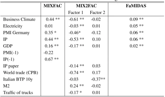
The estimated maximum likelihood parameters are listed in Table 1, whereas the monthly indicators are shown in Figure 1. In addition, Figure 2 shows the estimated GDP in monthly growth rates and the common factors for the three models. The graph clearly shows that the FaMIDAS produces a smoother factor which is a desirable property, and not surprising given that it sums over time lags. Similarly, the disaggregated monthly GDP from the FaMIDAS is more stable than the same obtained by the other two mixed frequency models (MIXFAC and MIX2FAC). Moreover, the confidence bands of the predictions, shown as fan charts in Figure 3, reveal smaller incertitude in the FaMIDAS model than in the other mix-frequency formulations.
The inspection of the spectral density of the estimated monthly GDP for the MIDAS and MIXFAC, shown in Figure 4, suggests that the FaMIDAS structure is able to capture standard business cycle frequencies and, therefore, might perform better in short-term forecasting than in nowcasting. Analyzing the minor volatility in terms of spectrum of frequencies, it turn out that the FaMIDAS picks up the less volatile components of the spectrum and thus the estimates are less affected by the noise of data revisions that occur in real time analysis. Indeed the fact that previsions from the FaMIDAS are less volatile makes them particularly useful for dealing with real time data which are subject to revision and, therefore, suffer for high degree of uncertainty.
The forecasting performance analysis of the three models requires an empirical applica-tion, which is presented in the next section. The deep treatment of the temporal disaggrega-tion in sample, and thus of the producdisaggrega-tion of a monthly measure of GDP, is left for future research.
4
Forecasting evaluation
In this section the three models under analysis are compared with respect to their forecasting ability, with a rolling experiment in a window of the latest 5,4,3 years up to the end of 2007
4. The rolling exercise is made in pseudo-real time, so as to mimic the delay of different
in-dicators, which has been proved to be relevant for correctly assessing which model performs
4We prefer to exclude the biennium 2008-2009 from the sample to avoid that the exceptional conditions of the economic crisis affect the results. In addition, at the time of writing, data from 2008 upwards were still preliminary and subject to revision.
best. Therefore the forecasting evaluation is made with specification of the month of the pre-diction inside the quarter (e.g. first month, second or third), which corresponds to a different information set. It is worth stressing that the Kalman filter is particularly suitable for this issue given that it solves endogenously the problem of the unbalanced sample produced by the difference in timing of publication of the monthly indicators. Consider the example of making a forecast for GDP the 1st of January 2010. The last GDP data available is the third quarter of 2009 so one needs to first estimate the value of GDP for the last quarter of 2009 and then make a prevision for the first and second quarter of 2010. Analogously, monthly indicators are published with a certain delay. In January, for example, we would have soft indicators, such as PMI or Business climate, for December 2009, while Industrial production for November 2009 would be release around the 15 of January 2010. Therefore indicators need to be forecasted for closing the quarter that should be predicted so as to balance the sample.
The Kalman filter allows doing this step endogenously as it solves directly the ragged-edge data issue by using the prediction routine. Moreover, every time a new observation for an indicator is released, all the series are generally revised for prior years and the MIDAS component helps reducing the statistical noise of the revisions in real time.
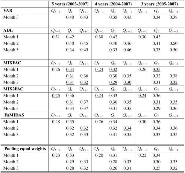
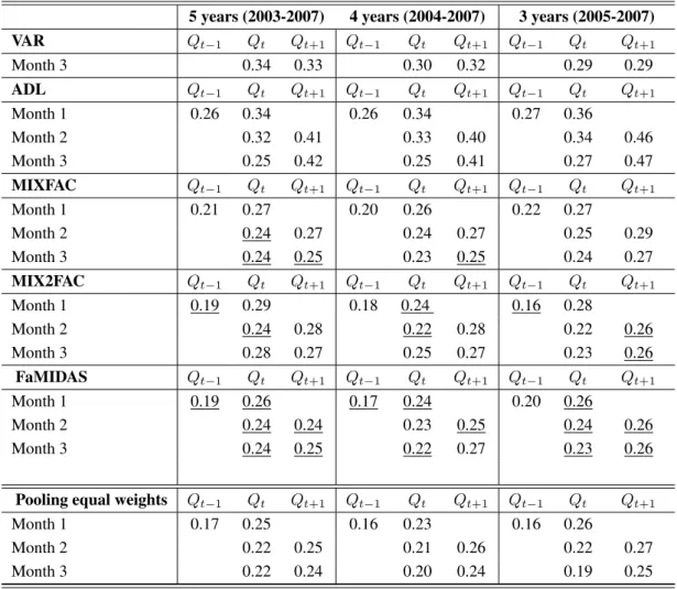
In Table 2 we show RMSE of the three mixed frequency factor models and of two ad-ditional benchmark models. To disentangle the role of the mixed frequency structure, we also consider a quarterly VAR (estimated with order 2 on the bases of the AIC criteria) that includes the same information set as the MIXFAC. Moreover, to assess the gain of the mul-tivariate structure we consider a univariate ADL modified as in Proietti (2004) to replicate a mixed frequency structure. We see that all the mixed frequency multivariate models easily outperform the other two benchmark models. Considering, in particular, the three mixed frequency models, we see that the differences in predictive ability are small and the ranking changes with the sample. The ranking is also subject to the loss function. For the case of a linear specification we see (Table 3) that the absolute value of the forecast errors are al-most always smaller for the FaMIDAS. Looking jointly at RMSE and MAPE, it seems that the MIX2FAC is more suited for nowcasting with complete information, while MIXFAC is better in nowcasting when the indicators are not known. FaMIDAS makes the lowest RMSE for one quarter-ahead when the information set is small (second month of the quarter). This last empirical evidence seems to reinforce the idea that the FaMIDAS exploit efficiently the correlation of the lag structure of the indicators with the target variable.
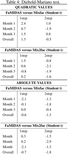
More generally, given the apparent absence of clear dominance of one model, we per-formed the DMW tests (Diebold, Mariano and West (1996)) of equal forecast ability to check if the ranking showed by RMSE is statistically significant. In particular, we tested the
hypothesis that FaMIDAS has the same predictive information as the other two models. The results, in Table 4, show that by using a quadratic loss function FaMIDAS is dominated by MIXFAC in nowcasting, but is significantly better than MIX2FAC in forecasting. However, when errors are considered in absolute values, FaMIDAS dominates also in nowcasting.
Since the seminal paper by Bates and Granger (1969), it is well know that combining different models results in a smaller forecast error than selecting a single specification. The general idea is that the combination of different specifications, by averaging, mitigate the model misspecification, instability and estimation error of each specific model (Timmermann 2006). Therefore, the pooling forecast is particularly suitable when the combined models show significant heterogeneity.
The application presented above matches this requirement, given that the models differ in terms of components (number of factors and lags), as well as for the best forecast horizon. In the bottom panel of Table 2 and Table 3 we report the real time errors for the pooled model with equal weights. The combination of the three models, the MIXFAC, MIX2FAC and FaMIDAS is preferred to each of them singularly and especially for quadratic errors. In fact, the forecasts produced by the pooling of different models dominates the single models more often for the RMSE than for the MAPE.5. A more proper combination would require
a dedicated analysis that we leave for future research. To conclude on this empirical appli-cation, we find that that the mixed frequency factor models regularly outperform standard VAR and univariate mixed frequency ADL. The differences in the forecasting ability of the three factor models are small, time dependent and not always statistically significant. In general, it emerges that MIXFAC and MIX2FAC appear more suited for nowcasting, while FaMIDAS seems better for forecasting. Nothwitstanding the small differences in RMSE a forecast combination of the three factor models reduces further the error, likely thanks to the heterogeneity in the structure of the three models.
5
Conclusions
The short-term forecasting literature has shown an increasing interest in mixed frequency models. These models are particularly useful in real time forecasting as they deal with the unbalanced data set problem and they reduce the temporal aggregation bias created by the different frequencies of the observable indicators. In this paper we combine two approaches: dynamic mixed frequency factor models and MIDAS. Our model, that we call FaMIDAS, is
5Although the simple average of forecast is not optimal, under general circumstances and symmetric loss functions it can generate a smaller loss (see Elliott and Timmermann (2004))
designed for applications in real time as it reduces the problem of the unbalanced data set and it is less affected by revisions of preliminary data. Moreover it can take into account changes over time of the leading power of timely high frequency indicators used for forecasting.
As by product we obtain a monthly index of GDP which is per-se relevant for business cycle analysis, as for example for defining a chronology of the cycle, which we left as future research.
In the empirical application we test the FaMIDAS against benchmark models and mixed frequency factor models with different structures. Overall the FaMIDAS produces smoother estimates for the disaggregate target variable and better forecasts over a longer horizon. In order to reduce further the prediction error a simple pooling is proposed.
Appendix: The State space representation and temporal
ag-gregation
Consider the factor model proposed in section 2.3:
yt = " b(Lk, θ)xt y2,t # = ϑ0ft+γt+Stβ, t= 1, ..., n, φ(L)∆ft = ηt, ηt ∼NID(0, ση2), D(L)∆γt = δ+η∗t, η∗t ∼NID(0,Ση∗). (3)
whereb(Lk, θ)xtis the MIDAS polynomial for the combination of lags of the monthly
eco-nomic indicators andy2,tis the aggregated variable that gathers the flow subject to temporal
aggregation ( e.g. the quarterly GDP). D(L) is a matrix containing autoregressive loading of the idyosincratics components. The common factor and the idiosyncratic components fol-low standard autoregressive processes and thus the model can be easily casted in State Space Form (SSF).
Consider the standard way to recast in SSF a general AR(p) processφ(L)∆ft =ηtwith
φ(L) = (1−φ1L−φ2L2−...−φpLp): ft=e01,p+1αt, αt=Tfαt−1+Hηt, where αt= " ft ft∗ # , Tf = " 1 e01pTφ 0 Tφ # ,Tφ = φ1 .. . φp−1 Ip−1 φp 00 . andft∗ =Tφft∗−1+e1pηt,H= [1,e01,p] 0,e 1p = [1,0, . . . ,0]0 .
And then apply the previous representation to the common factor and each idiosyncratic. The SSF of the complete model results:
yt= " b(Lk, θ)xt y2,t # =Zαt+Stβ, αt=Tαt−1+Wb+Ht, (4)
where the state vector and the vector of errors are obtained stacking the single SSF represen-tation of the autoregressive processes, namely:[αt =α0f,t, α0γ1,t, . . . , α
0 γN,t]
0, for the state and
t= [ηt, η1∗,t, . . . , ηN,t∗ ]0 for the vector of errors.
The system matrices of the measurement equation become:
Z = θ0, ... θ1 ... 0... diag(e0p1, . . . ,e 0 pN) , T=diag(Tf,Tγ1, . . . ,TγN), H=diag(Hf,Hγ1, . . . ,HγN). (5)
The matrixWis time invariant and selects the driftδifor the appropriate state element of
the idiosyncratic component.
The temporal aggregation problem is solved following the strategy proposed by Harvey (1989). The block of variables subject to temporal aggregation,y2, are replaced by anad hoc cumulator variable,y2c,t, defined so that it coincides with the (observed) aggregated series at the end of the larger interval (e.g. quarter), otherwise it contains the partial cumulative value of the aggregate in the seasons (e.g. months), as follow:
yc2,t =ψtyc2,t−1+y2,t, ψt = (
0 t=δ(τ −1) + 1, τ = 1, . . . ,[n/δ] 1 otherwise,
The cumulator is used to replace the second block of the measurement equation and to augment the state equation as follow:
α∗t = " αt yc 2,t # , y†t = " b(Lk, θ)xt yc 2,t #
The final measurement and transition equation are therefore:
yt†=Z∗α∗t +Stβ, α∗t =T ∗
α∗t−1+W∗β+H∗t, (6)
with system matrices:
Z∗ = " Z1 0 0 IN2 # , T∗ = " T 0 Z2T ψtI # , W∗ = " W Z2W+S2 # , H∗ = " I Z2 # H. (7)
References
Altissimo, F., Cristadoro , R., Forni M., Lippi M.,Veronese G. (2007). New Eurocoin: Tracking Economic Growth in real time, Bank of Italy working paper n. 631.
Andreou E., Ghysel E. , and A. Kourtellos, (2009), “Should macroeconomic forecasters use daily financial data and how?”, UNC Working Paper.
Aruoba, S. B., F. X. Diebold, and C. Scotti, (2009), “Real-time Measurement of Business Conditions”,Journal of Business & Economic Statistics27 (4).
Barhoumi, K., S. Benk, R. Cristadoro, A. D. Reijer, A. Jakaitiene, P. Jelonek, A. Rua, G. R¨unstler, K. Ruth, and C. V. Nieuwenhuyze (2009). “Short-term forecasting of GDP using large monthly datasets: a pseudo real-time forecast evaluation exercise”,Journal of Forecasting28 (7).
Bates, J.M., C.W.J. Granger, (1969), “The combination of forecasts”,Operations Research Quarterly20.
Camacho, M., and G. Perez-Quiros, (2009), “Introducing the Euro-Sting: short term indi-cator of the Euro Area growth”, CEPR Discussion Paper No. 7343. Available at SSRN: http://ssrn.com/abstract=1461972
Clements, M. P., and A. B. Galv˜ao, (2008), “Macroeconomic forecasting with mixed fre-quency data”,Journal of Business and Economic Statistics26(4).
Clements, M. P., and A. B. Galv˜ao, (2010), “Real-time Forecasting of Inflation and Output growth in the Presence of data Revisions”, manuscript.
Doornik, J.A., (2001),Ox 3.0 - An Object-Oriented Matrix Programming Language, Tim-berlake Consultants Ltd: London.
Drechsel, K., and L. Maurin, (2008), “Flow of conjunctural information and forecast of the Euro Area Economic Activity”, ECB Working Paper No. 925. Available at SSRN: http://ssrn.com/ abstract=1188603
Elliott, G., Granger, C. and Timmermann, A., “ Handbook of economic forecasting”, Else-vier edition 1, volume 1, number 1, December.
Elliott, G., and Timmermann, A., (2004), “Optimal forecast combinations under general loss function and forecast error distribution”, Journal of Econometrics, Elsivier, vol. 122(1).
Frale, C., M. Marcellino, G. L. Mazzi, T. Proietti, (2008), “A monthly indicator of the Euro Area GDP”, CEPR Discussion Paper No. 7007. Available at SSRN: http://ssrn.com/ abstract=1311131
Ghysels, E., P. Santa-Clara, and R. Valkanov, (2002), “The MIDAS touch: mixed data sampling regression models”, UNC and UCLA Working Papers.
Ghysels, E., P. Santa-Clara, and R. Valkanov, (2006), “Predicting volatility: getting the most out of return data sampled at different frequencies”,Journal of Econometrics131(1-2). Harvey, A.C., (1989), Forecasting, structural time series models and the Kalman filter,
Cambridge University Press: Cambridge.
Harvey, A.C., and C.H. Chung, (2000), “Estimating the underlying change in unemploy-ment in the UK”,Journal of the Royal Statistics Society Series A, 163(3).
Koopman, S.J., and J. Durbin, (2000), “Fast filtering and smoothing for multivariate state space models”,Journal of Time Series Analysis, 21(3).
Marcellino, M. (1999), “Some consequences of temporal aggregation in empirical analy-sis”, Journal of Business and Economic Statistics 11.
Marcellino, M., and C. Schumacher, (2008), “Factor-MIDAS for now- and forecasting with ragged-edge data: a model comparison for German GDP”, CEPR Discussion Paper No. 6708.
Mariano, R.S., and Y. Murasawa, (2003), “A new coincident index of business cycles based on monthly and quarterly series”,Journal of Applied Econometrics18(4).
Mittnik, S., and P. Zadrozny, (2004), “Forecasting quarterly German GDP at monthly inter-vals using monthly IFO Business Conditions data”, CESifo Working Paper No. 1203. Moauro, F., and G. Savio , (2005), “Temporal disaggregation using multivariate structural
time series models”,Econometrics Journal8(2).
Monteforte, L., and G. Moretti, (2009), “Real time forecasts of inflation: the role of finan-cial variables”, LUISS Lab Working Paper, No. 81.
Proietti, T., (2006), “Temporal disaggregation by state space methods: Dynamic regression methods revisited”,Econometrics Journal9(3).
Proietti T. and Moauro F. (2006). Dynamic Factor Analysis with Nonlinear Temporal Ag-gregation Constraints. Journal of the Royal Statistical Society, series C (Applied Statis-tics), 55, 281300.
Stock, J.H., and M.W. Watson, (1999), “A comparison of linear and nonlinear univariate models for forecasting macroeconomic time series”, in Engle, R. and White, R. (eds),
Cointegration, causality and forecasting: A festschrift in honor of Clive W.J. Granger, Oxford: Oxford University Press.
Timmermann, A. G. (2006). “Forecast combinations”. In Handbook of Economic Fore-casting, G. C. W. J. Elliot, G and A. Timmermann, eds., vol. 1. Amsterdam: Elsevier. West, K.D., (1996), “Asymptotic Inference About Predictive Ability”, Econometrica, 64.
Table 1: Estimated factor loadings
MIXFAC MIX2FAC FaMIDAS
Factor 1 Factor 2 Business Climate 0.44 ** -0.61 ** -0.02 0.09 ** Electricity 0.01 -0.03 ** 0.01 0.05 ** PMI Germany 0.35 * -0.46* -0.12 0.06 ** IP 0.44 ** -0.53 ** 0.10 0.06 ** GDP 0.16 ** -0.17 ** 0.01 0.02 ** PMI(-1) -0.22 IP(-1) 0.67 ** IP paper -0.14 ** 0.03 World trade (CPB) -0.74 ** 0.17 Italian BTP 10y -0.03 -0.37** M2 0.24 ** -0.02 Traffic of trucks -0.17 * 0.01 ** Means significant at 5%, * at 10%.
The sample period range from 1990M1 to 2009M4. Business Climate is provided by ISAE; Electricity is the monthly consumption of electricity provided by TERNA; PMI Germany is the Purchase Manager Index for Germany in manufacturing and services; IP paper is the Industrial production of paper and cardboard; World trade is the indica-tor of trade produced by the CPB- Netherlands Bureau for Economic Policy Analysis; Money supply includes currency and deposits; Motorway flow refers to trucks and is provided by Autostrade
Table 2: Rolling forecasting experiment: RMSE.
5 years (2003-2007) 4 years (2004-2007) 3 years (2005-2007) VAR Qt−1 Qt Qt+1 Qt−1 Qt Qt+1 Qt−1 Qt Qt+1 Month 3 0.40 0.43 0.35 0.43 0.34 0.38 ADL Qt−1 Qt Qt+1 Qt−1 Qt Qt+1 Qt−1 Qt Qt+1 Month 1 0.31 0.42 0.30 0.42 0.30 0.43 Month 2 0.40 0.45 0.40 0.46 0.41 0.50 Month 3 0.34 0.45 0.33 0.46 0.33 0.50 MIXFAC Qt−1 Qt Qt+1 Qt−1 Qt Qt+1 Qt−1 Qt Qt+1 Month 1 0.26 0.34 0.24 0.32 0.26 0.35 Month 2 0.31 0.36 0.30 0.35 0.32 0.38 Month 3 0.31 0.32 0.29 0.30 0.31 0.32 MIX2FAC Qt−1 Qt Qt+1 Qt−1 Qt Qt+1 Qt−1 Qt Qt+1 Month 1 0.25 0.36 0.24 0.33 0.24 0.36 Month 2 0.31 0.37 0.30 0.35 0.31 0.35 Month 3 0.34 0.37 0.31 0.35 0.29 0.36 FaMIDAS Qt−1 Qt Qt+1 Qt−1 Qt Qt+1 Qt−1 Qt Qt+1 Month 1 0.28 0.35 0.26 0.34 0.30 0.36 Month 2 0.32 0.32 0.32 0.34 0.34 0.36 Month 3 0.32 0.33 0.31 0.35 0.33 0.35
Pooling equal weights Qt−1 Qt Qt+1 Qt−1 Qt Qt+1 Qt−1 Qt Qt+1
Month 1 0.23 0.33 0.20 0.31 0.22 0.34
Month 2 0.29 0.33 0.28 0.33 0.30 0.35
Month 3 0.28 0.32 0.26 0.31 0.25 0.32
Note: Each entry represents the RMSE of the rolling forecast of GDP growth rates, aggregated to the quarterly frequency, by month of the quarter in which the prevision is made, horizon of prevision and window length. The best values among the models (except for the pooling) are underlined. The VAR is estimated on a balanced quarterly sample. The ADL is estimated as documented by Proietti (2006) by using the routines provided by the author
Table 3: Rolling forecasting experiment: MAE.
5 years (2003-2007) 4 years (2004-2007) 3 years (2005-2007) VAR Qt−1 Qt Qt+1 Qt−1 Qt Qt+1 Qt−1 Qt Qt+1 Month 3 0.34 0.33 0.30 0.32 0.29 0.29 ADL Qt−1 Qt Qt+1 Qt−1 Qt Qt+1 Qt−1 Qt Qt+1 Month 1 0.26 0.34 0.26 0.34 0.27 0.36 Month 2 0.32 0.41 0.33 0.40 0.34 0.46 Month 3 0.25 0.42 0.25 0.41 0.27 0.47 MIXFAC Qt−1 Qt Qt+1 Qt−1 Qt Qt+1 Qt−1 Qt Qt+1 Month 1 0.21 0.27 0.20 0.26 0.22 0.27 Month 2 0.24 0.27 0.24 0.27 0.25 0.29 Month 3 0.24 0.25 0.23 0.25 0.24 0.27 MIX2FAC Qt−1 Qt Qt+1 Qt−1 Qt Qt+1 Qt−1 Qt Qt+1 Month 1 0.19 0.29 0.18 0.24 0.16 0.28 Month 2 0.24 0.28 0.22 0.28 0.22 0.26 Month 3 0.28 0.27 0.25 0.27 0.23 0.26 FaMIDAS Qt−1 Qt Qt+1 Qt−1 Qt Qt+1 Qt−1 Qt Qt+1 Month 1 0.19 0.26 0.17 0.24 0.20 0.26 Month 2 0.24 0.24 0.23 0.25 0.24 0.26 Month 3 0.24 0.25 0.22 0.27 0.23 0.26
Pooling equal weights Qt−1 Qt Qt+1 Qt−1 Qt Qt+1 Qt−1 Qt Qt+1
Month 1 0.17 0.25 0.16 0.23 0.16 0.26
Month 2 0.22 0.25 0.21 0.26 0.22 0.27
Month 3 0.22 0.24 0.20 0.24 0.19 0.25
Note: Each entry represents the MAE of the rolling forecast of GDP growth rates, aggregated to the quarterly frequency, by month of the quarter in which the prevision is made, horizon of prevision and window length. The best values among the models (except for the pooling) are underlined. The VAR is estimated on a balanced quarterly sample. The ADL is estimated as documented by Proietti (2006) by using the routines provided by the author
Table 4: Diebold-Mariano test.
QUADRATIC VALUES FaMIDAS versus Mixfac (Student t)
1step 2step
Month 1 2.4 1.0
Month 2 0.7 -1.9
Month 3 1.5 0.8
Overall 1.3 -0.5
FaMIDAS versus Mix2fac (Student t)
1step 2step Month 1 1.5 -0.8 Month 2 0.6 -2.1 Month 3 -0.8 -1.9 Overall 0.2 -1.6 ABSOLUTE VALUES FaMIDAS versus Mixfac (Student t)
1step 2step
Month 1 -2.1 -1.3
Month 2 -0.1 -1.8
Month 3 0.0 -0.4
Overall -0.6 -1.3
FaMIDAS versus Mix2fac (Student t)
1step 2step
Month 0.3 -1.5
Month 0.2 -2.9
Month -2.1 -1.3
Overall -0.7 -1.8
Note: The test of equal forecasting abil-ity is made by horizon of previsions and month in the quarter based on a rolling forecast window of 5 years on the range 2003-2007. Student-T values are adjusted by using the Newey-West correction.
Figure 1: Monthly Indicators and Quarterly GDP- Italy 1990 1993 1996 1999 2002 2005 2008 60 80 100 Business climate 1990 1993 1996 1999 2002 2005 2008 17.5 20.0 22.5 25.0 Electricity Consumption 1990 1993 1996 1999 2002 2005 2008 40 50
60 PMI Index Germany
1990 1993 1996 1999 2002 2005 2008 90 100 110 Industrial Production 1990 1993 1996 1999 2002 2005 2008 100 150 200 World trade 1990 1993 1996 1999 2002 2005 2008 275000 300000 325000 Quarterly GDP 1990 1993 1996 1999 2002 2005 2008 300000 350000 400000 Production of paper 1990 1993 1996 1999 2002 2005 2008 6000 7000 8000 9000 10000 11000 M2 1990 1993 1996 1999 2002 2005 2008 0.05 0.10 0.15 0.20 Italian BTP 10 y (deflated) 1990 1993 1996 1999 2002 2005 2008 100 120
Traffic of tracks (Index 2000=100)
2
Figure 2: Estimated Monthly GDP and common factors . 2000 2001 2002 2003 2004 2005 2006 2007 2008 2009 −0.010 −0.005 0.000 0.005
GDP Monthly Growth Rates
MIXFAC MIX2FACT FaMIDAS 1990 1992 1994 1996 1998 2000 2002 2004 2006 2008 0 25 50 Common Factor MIXFAC MIX2FACT−Factor 1 FaMIDAS MIX2FACT−Factor 2 1990 1991 1992 1993 1994 1995 1996 1997 1998 1999 2000 −0.010 −0.005 0.000 0.005 0.010
Figure 3: Forecasts and fan charts 2006 2007 2008 106000 108000 110000 FaMIDAS 2006 2007 2008 MIX2FAC 2006 2007 2008 MIXFAC 2 4
Figure 4: Spectral Density of the Monthly GDP. 0.0 0.2 0.4 0.6 0.8 1.0 0.0 0.2 0.4 0.6 0.8 1.0 0.0 0.2 0.4 0.6 0.8 1.0 0.1 0.2 0.3 0.4 0.5 0.6 0.7 0.8 0.9 1.0 Spectral density MIXFAC MIX2FAC FaMIDAS
Note: The horizontal axis represents frequencies from 0 to𝜋, while on the vertical axis the estimated spectral density of the monthly GDP in growth rates.
Ministry of Economy and Finance
Directorate I: Economic and Financial Analysis
Address: Via XX Settembre, 97 00187 - Rome Websites: www.mef.gov.it www.dt.tesoro.it e-mail: [email protected] Telephone: +39 06 47614202 +39 06 47614197 Fax: +39 06 47821886