Bracket creep and deadweight from California's state income tax, 1958-1977

(1)

Calhoun: The NPS Institutional Archive

Theses and Dissertations Thesis Collection

2002-06

Bracket creep and deadweight from California's

state income tax, 1958-1977

Neal, Erik J.

Monterey, California. Naval Postgraduate School

(2)

NAVAL POSTGRADUATE SCHOOL

Monterey, California

THESIS

BRACKET CREEP AND DEADWEIGHT FROM CALIFORNIA’S STATE INCOME TAX, 1958-1977

by

Erik J. Neal June 2002

Thesis Advisor: David R. Henderson Co-Advisor: Raymond E. Franck

(3)

(4)

REPORT DOCUMENTATION PAGE

Form Approved OMB No. 0704-0188

Public reporting burden for this collection of information is estimated to average 1 hour per response, including the time for reviewing instruction, searching existing data sources, gathering and maintaining the data needed, and completing and reviewing the collection of information. Send comments regarding this burden estimate or any other aspect of this collection of information, including suggestions for reducing this burden, to Washington headquarters Services, Directorate for Information Operations and Reports, 1215 Jefferson Davis Highway, Suite 1204, Arlington, VA 22202-4302, and to the Office of Management and Budget, Paperwork Reduction Project (0704-0188) Washington DC 20503.

1. AGENCY USE ONLY (Leave

blank) 2. REPORT DATEJune 2002 3. REPORT TYPE AND DATES COVEREDMaster’s Thesis

4. TITLE AND SUBTITLE Title

Bracket Creep and Deadweight Loss from California’s State Income Tax, 1958-1977

5. FUNDING NUMBERS 6. AUTHOR (S) Erik J. Neal

7. PERFORMING ORGANIZATION NAME(S) AND ADDRESS(ES) Naval Postgraduate School

Monterey, CA 93943-5000

8. PERFORMING ORGANIZATION REPORT NUMBER

9. SPONSORING / MONITORING AGENCY NAME(S) AND ADDRESS(ES)

N/A 10. SPONSORING/MONITORING AGENCY REPORT NUMBER 11. SUPPLEMENTARY NOTES The views expressed in this thesis are those of the author and do not reflect the official policy or position of the U.S. Department of Defense or the U.S. Government.

12a. DISTRIBUTION / AVAILABILITY STATEMENT

Approved for public release; distribution is unlimited 12b. DISTRIBUTION CODE

13. ABSTRACT (maximum 200 words)

This thesis shows that a combination of "bracket creep" and legislated tax rate increases during the Edmund G. “Pat” Brown and Ronald Reagan governorships caused individual marginal tax rates to increase as much as 600 percent. A person earning $20,000 in 1958 was in the three percent bracket for state income taxes. Assuming this person received no real pay raises, his inflation-adjusted income in 1977 was now $41,938 and his marginal tax bracket was 11 percent. This person experienced a 355 percent increase in real taxes paid.

The deadweight loss calculations show how bracket creep and legislated tax rate increases exacerbate deadweight loss. The more revenue the federal or state government tries to collect, the more deadweight loss society as a whole incurs. Using elasticities (of taxable income with respect to tax rates) ranging from .3 to 1.0, the incremental deadweight loss as a percent of incremental revenue collected from 10.6 percent for an elasticity of .3, to as high as 35.53 percent for an elasticity of 1.0. The deadweight loss calculations show that for every dollar in revenue collected, at least 10.7 cents to as much as 35.5 cents per dollar is lost to deadweight loss.

14. SUBJECT TERMS

Bracket Creep and Deadweight Loss

15. NUMBER OF PAGES 48 16. PRICE CODE 17. SECURITY CLASSIFICATION OF REPORT Unclassified 18. SECURITY CLASSIFICATION OF THIS PAGE Unclassified 19. SECURITY CLASSIFICATION OF ABSTRACT Unclassified 20. LIMITATION OF ABSTRACT UL NSN 7540-01-280-5500 Standard Form 298 (Rev. 2-89) Prescribed by ANSI Std. 239-18

(5)

(6)

Approved for public release; distribution is unlimited BRACKET CREEP AND DEADWEIGHT LOSS FROM CALIFORNIA’S STATE

INCOME TAX, 1958-1977 Erik J. Neal

Lieutenant, United States Navy B.A., Seattle University, 1996

Submitted in partial fulfillment of the requirements for the degree of MASTER OF SCIENCE IN MANAGEMENT

from the

NAVAL POSTGRADUATE SCHOOL June 2002

Author: Erik J. Neal

Approved by: David R. Henderson Principal Advisor Raymond E. Franck Associate Advisor

Douglas A. Brooke, Ph.D.

Dean, Graduate School of Business and Public Policy

(7)

(8)

ABSTRACT

This thesis shows that a combination of "bracket creep" and legislated tax rate increases during the Edmund G. “Pat” Brown and Ronald Reagan governorships caused individual marginal tax rates to increase as much as 600 percent. A person earning $20,000 in 1958 was in the three percent bracket for state income taxes. Assuming this person received no real pay raises, his inflation-adjusted income in 1977 was now $41,938 and his marginal tax bracket was 11 percent. This person experienced a 355 percent increase in his marginal tax rate.

The deadweight loss calculations show how bracket creep and legislated tax rate increases exacerbate deadweight loss. The more revenue the federal or state government tries to collect, the more deadweight loss society as a whole incurs. Using elasticities (of taxable income with respect to tax rates) ranging from .3 to 1.0, the incremental deadweight loss as a percent of incremental revenue collected ranged from 10.6 percent for an elasticity of .3, to as high as 35.53 percent for an elasticity of 1.0. The deadweight loss calculations show that for every dollar in revenue collected, at least 10.7 cents to as much as 35.5 cents per dollar is lost to deadweight loss.

(9)

(10)

LIST OF FIGURES

Figure 3.1. Labor Market at Equilibrium...22 Figure 3.2. Labor Market with FIT...23 Figure 3.3. Labor Market with FIT and SIT...24

(13)

(14)

LIST OF TABLES

Table 2.1. The Effects of Bracket Creep for Married Filing Joint Returns...10 Table 2.2. Married Persons Filing Joint Returns...10 Table 2.3. Single and Married Persons Filing Separate

Returns...12 Table 2.4. Unmarried Heads of Household...13 Table 2.5. CPI-U. [Ref: Consumer Price Index, 1913-2002....17 Table 3.1. Deadweight Loss from State Taxes with an

Elasticity of .3...26 Table 3.2. Deadweight Loss from State Taxes with an

(15)

(16)

I. INTRODUCTION

A. OVERVIEW

This thesis studies the California income tax system from 1935 to 2001—specifically, the marginal tax rates at various real-income levels, taking into account the interaction between the state and federal tax systems.

B. RESEARCH QUESTIONS

This thesis explains and answers the following questions:

• Why are California’s income tax rates so high?

• How has inflation affected marginal income tax bracket creep?

• What is the deadweight loss (the loss to society) caused by high tax rates?

C. DISCUSSION

One of the major factors affecting economic activity in a location is that location’s tax system. All other things equal, the lower the tax rate in an area, the more attractive the area is for economic activity. This matters for location across states because movement from one state to another is relatively low cost. The fact that workers can move from California to Nevada, for example, means that wages net of taxes will tend to equalize, which means that wages net of taxes will tend to be higher in the high-tax-rate state. This fact, in turn, means that production will be more expensive in the high-tax state. This is particularly relevant for defense production—and even for location of military bases—because the Department of Defense (DoD) often has the option of choosing one state over another.

(17)

It becomes important, therefore, to understand the tax systems of various states. California’s tax system is particularly important to understand because California’s economy is the fifth-largest in the world. [Ref. 1]

D. SCOPE OF THE THESIS

This thesis includes: (1) historical income tax tables from 1935 to 2001; (2) a narrative of three time periods in California’s history—Governors Earl Warren’s, Pat Brown’s and Ronald Reagan’s administrations; (3) an inflation adjustment to the tax tables showing bracket creep and the impact on marginal tax rates for the people at various real income levels; and (4) an estimate of the deadweight loss of California’s income tax system, based on California taxes and on the interaction between the state and federal tax systems.

E. METHODOLOGY

• Compile California income tax tables from 1935 to 2001.

• Provide an historical perspective on California state taxes.

• Calculate income tax rate bracket creep.

• Use elasticities of taxable income with respect to tax rates to calculate deadweight loss from high tax rates.

F. ORGANIZATION OF THESIS

Chapter II provides the background for this thesis by: (1) describing the income tax system and how it has evolved; (2) providing historical income tax tables from 1935 to 2001; (3) providing an historical narrative of three governors, their tenures, and their effect on taxes; and (4) adjusting tables for inflation (bracket creep). Chapter III calculates the deadweight loss from the

(18)

California state income tax system. Chapter IV states a conclusion.

(19)

(20)

II. THE EVOLUTION OF CALIFORNIA’S STATE INCOME

TAXES

A. BACKGROUND

Prior to 1935, local governments in California relied primarily on property taxes for revenue. The Great Depression of the 1930s was the single most significant event that led to adoption of sales and state income taxes. During the Depression, property owners found it increasingly difficult to pay their property taxes and sought relief by way of a voter referendum to change existing property tax laws.

Elementary and secondary school expenditures were mandated by the state and paid with local property taxes. If property tax relief were to occur, the state would have to bear more of the fiscal burden. Proponents of property tax relief included Proposition 9 on the general election ballot of 08 November, 1932. The bill, if passed, would have provided property tax relief, but also would have permitted the introduction of sales and personal income taxes. [Ref. 2:p. 59] Proposition 9, which was poorly worded, was defeated by a vote of 1,144,449 to 552,738.

In 1933, the Great Depression was in full swing. California’s general fund surplus, funded by a gross receipts tax on utilities, was depleted, and the state’s first deficit was growing. Something had to be done. The governor’s ideas for fiscal recovery fell on deaf ears. Meanwhile, the legislature drafted its solution, the Riley-Stewart initiative.

(21)

The Riley-Stewart initiative, which the voters approved in a special election on 27 June 1933, had four main components: public utility property was to be returned to local property tax rolls and the gross receipts tax abolished in 1935; the state would provide additional support for elementary and secondary schools; limits were to be placed on expenditure increases both at the state and local level; and the Legislature was to be authorized to raise additional revenue to meet the cost for school aid. The source of this revenue was not described in the initiative but it was generally acknowledged that a sales tax would be necessary. [Ref. 2:p. 59]

The initiative was passed and gave rise to new problems. Now that the state was paying for school aid, the general fund deficit grew. In order to cover this new expense, the state adopted retail sales taxes and tried to adopt personal income taxes. Governor Sunny Jim Rolph vetoed the personal income taxes. It is important to note that the California State budget operated on a biennium.

After Rolph died in office, Frank Merriam succeeded him as governor and then won the nomination in 1934. Merriam inherited a large budget deficit and, by 1935, the budget deficit had increased even further. His solution was an increase in retail sales taxes from two percent to three percent and a personal income tax. [Ref. 2:p. 60) The Legislature approved his requests, and California residents have been paying personal income taxes since then.

B. THE EARL WARREN ERA

Earl Warren was elected in 1943 and served three consecutive terms. He inherited a state budget recovering from ten years of deficits (1931-1941). [Ref. 3:p. 7] World War II stimulated California’s economy, and, by 1943, the

(22)

general fund revenue-to-expenditure ratio was greater than one. Instead of increasing government spending, Governor Warren successfully advocated saving surpluses generated by the wartime economy. As the surplus grew, Warren cut sales taxes from three to two-and-one-half percent and the maximum personal income tax rate from fifteen to six percent. [Ref. 3:pp. 11-12] According to an article by David Doerr in the Cal-Tax Digest, “By 1947, the state had sequestered $472 million in various reserve funds for emergency use.” [Ref. 3:p. 12] California state tax laws remained relatively unchanged until 1959, when Edmond G. “Pat” Brown took office.

C. THE EDMOND G. “PAT” BROWN ERA

Edmond G. “Pat” Brown became governor on January 5, 1959. The surpluses accrued by Governor Warren had been used up during the years from 1955 through 1958. During this time there were gross imbalances between revenue and expenditures caused by an increase in state funding for education. The legislature chose not to raise personal income taxes or sales taxes; however, it did raise taxes on gasoline and car registrations from four-and-one-half cents to six cents per gallon and from six to eight dollars, respectively. The revenues generated were not enough to cover the entire cost of the increased expenditures on education, and the reserve funds, or surplus, accumulated under Governor Warren were depleted. [Ref. 3:p. 13]

Governor Brown faced budget deficits reminiscent of the Warren era. Republicans favored cutting government spending, but Brown chose to increase taxes. According to Doerr, “To fund his new budget, Governor Brown suggested a

(23)

$202 million tax increase, the largest such increase in nearly a quarter century.” [Ref. 4:p. 2] Central to his tax increases was the change to personal income taxes from the six-percent maximum set by Governor Warren to seven percent, the narrowing of tax brackets from $10,000 to $5000 for married couples filing jointly and from $5000 to $2500 for all others, and a reduction of personal exemptions. These changes were intended to produce $60.7 million dollars of revenue. [Ref. 4:p. 2] Personal income tax laws remained unchanged for the remainder of Brown's time in office.

D. THE RONALD REAGAN ERA

Ronald Reagan was elected Governor on January 2, 1967. Doerr describes the steps that Reagan took to cut government spending:

He first ordered a hiring freeze, a 10-percent budget cut of all state agencies, and other expenditure reductions. However, it soon became apparent that taxes would have to be raised substantially. Mr. Reagan was only able to slow the rate of growth of the state’s general fund expenditures only 8 percent from 1966-1967 to 1967-68, compared to 16 percent in the year prior). [Ref. 4:p. 2]

Reagan's actions were not enough, however, and he chose to raise taxes to cover the gap between expenditures and revenue. The maximum personal income tax was raised from seven to ten percent. Tax brackets were narrowed once again, from $5000 to $4000 for joint and single returns. Governor Reagan passed several other tax increases not related to personal income taxes; these are beyond the scope of this thesis and will not be addressed.

(24)

E. BRACKET CREEP

According to Taxopedia, a web-based tax information site, bracket creep occurs

when inflation pushes income into higher tax brackets. The result is no increase in real purchasing power but an increase in income tax payable. [Ref. 5]

Bracket creep, if left unchecked, is a crafty means by which federal, state or local governments can collect additional revenues from taxpayers without explicitly raising income tax rates.

Many features of personal income taxes are defined by fixed dollar amounts. For instance, income taxes have various rates starting at different dollar amounts of income. If these fixed amounts are not adjusted periodically, taxes can go up substantially simply because of inflation. Over time, bracket creep tends to reduce the real value of other important features of the tax system, such as exemptions and standard deductions, as well.

Table 2.1 illustrates the effects of bracket creep and legislated tax rate increases in California for different levels of income and calculates the percentage increase in real income and marginal tax rates from 1958 dollars to 1977 dollars. For example, a married person filing a joint return earning $5000 in 1958 would be in the one-percent tax bracket and pay $50 in state taxes for the year. That same $5000 in income equates to $10,484 in 1977 dollars. The $50 in taxes paid, inflation adjusted to 1977 dollars is now $105, assuming the person earned the same pay in real terms. He pays $209 in taxes in 1977. The percentage increase in real taxes paid is 100 percent, and the percentage increase in the marginal tax rate is 300

(25)

percent. This shows that a person making $5000 in 1958, assuming no increase in real pay, paid 100 percent more in state taxes on the same amount of income and experienced a 300-percent increase in his or her marginal tax rate.

Table 2.1. The Effects of Bracket Creep for Married Filing Joint Returns.

Married Filing Joint Returns Base

1958

adjusted From 1958 to1977 Year Income Tax rate Tax paid 77$ Income Tax rate Tax paid % incr in real tax % incr in MTR 1958 $5,000 1% $50 $105 $10,484 4% $209 100% 300%

$10,000 1% $100 $209 $20,969 7% $778 271% 600% $20,000 3% $300 $629 $41,938 11% $2863 355% 267% $30,000 3% $600 $1258 $62,907 11% $5170 311% 267%

The following tables are the historical personal income tables for California from 1935 to 1993 and the consumer price index from 1913 to 2001. These tables were used for the calculations in Table 2.1.

Table 2.2. Married Persons Filing Joint Returns.

Taxable Income

(adjusted gross income less Taxable Year

deductions and exemptions) 1935-42 1943-48a 1949-51 1952-58b 1959-66c Up to $2,500 1.0% 1.0% 1.0% 1.0% 1.0% $2,500 to 5,000 1.0 1.0 1.0 1.0 1.0 5,000 to 7,500 2.0 1.0 2.0 1.0 2.0 7,500 to 10,000 2.0 1.0 2.0 1.0 2.0 10,000 to 12,500 3.0 2.0 3.0 2.0 3.0 12,500 to 15,000 3.0 2.0 3.0 2.0 3.0 15,000 to 20,000 4.0 3.0 4.0 2.0 4.0 20,000 to 25,000 5.0 4.0 5.0 3.0 5.0 25,000 to 30,000 6.0 5.0 6.0 3.0 6.0 30,000 to 40,000 7.0 6.0 6.0 4.0 7.0 40,000 to 50,000 8.0 6.0 6.0 5.0 7.0 50,000 to 60,000 9.0 6.0 6.0 6.0 7.0 60,000 to 70,000 10.0 6.0 6.0 6.0 7.0 70,000 to 80,000 11.0 6.0 6.0 6.0 7.0 80,000 to 100,000 12.0 6.0 6.0 6.0 7.0 100,000 to 150,000 13.0 6.0 6.0 6.0 7.0 150,000 to 250,000 14.0 6.0 6.0 6.0 7.0 250,000 and over 15.0 6.0 6.0 6.0 7.0

(26)

Taxable Year

Taxable Income* 1967-72d 1973e,f

Up to $4,000 1.0% 1.0% $4,000 to 7,000 2.0 2.0 7,000 to 10,000 3.0 3.0 10,000 to 13,000 4.0 4.0 13,000 to 16,000 5.0 5.0 16,000 to 19,000 6.0 6.0 19,000 to 22,000 7.0 7.0 22,000 to 25,000 8.0 8.0 25,000 to 28,000 9.0 9.0 28,000 to 31,000 10.0 10.0 31,000 and over 10.0 11.0

Taxable Income* Taxable Year 1986

Up to $3,420 0% $3,420 to 10,420 1 10,420 to 15,620 2 15,620 to 20,840 3 20,840 to 26,160 4 26,160 to 31,420 5 31,420 to 36,660 6 36,660 to 41,860 7 41,860 to 47,120 8 47,120 to 52,360 9 52,360 to 57,580 10 57,580 and over 11

Taxable Income* Taxable Year 1987-90g

Up to 7,300 1.0% 7,300 to 17,300 2.0 17,300 to 27,300 4.0 27,300 to 37,900 6.0 37,900 to 47,900 8.0 47,900 and over 9.3

Taxable Income* Taxable Year 1991-92h

Up to $8,788 1.0% $8,788 to 20,828 2.0 20,828 to 32,870 4.0 32,870 to 45,632 6.0 45,632 to 57,670 8.0 57,670 to 200,000 9.3 200,000 to 400,000 10.0 400,000 and over 11.0

Up to $9,332 1.0% $9,332 to 22,118 2.0 22,118 to 34,906 4.0 34,906 to 48,456 6.0 48,456 to 61,240 8.0 61,240 to 212,380 9.3

(27)

212,380 to 424,760 10.0

424,760 and over 11.0

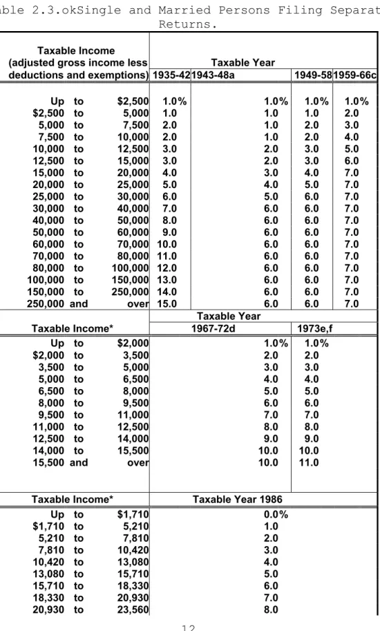
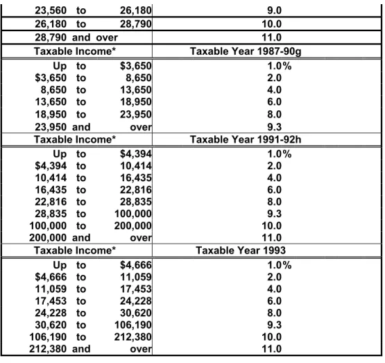
Table 2.3.okSingle and Married Persons Filing Separate Returns.

Taxable Income (adjusted gross income less Taxable Year deductions and exemptions) 1935-421943-48a 1949-58 1959-66c

Up to $2,500 1.0% 1.0% 1.0% 1.0% $2,500 to 5,000 1.0 1.0 1.0 2.0 5,000 to 7,500 2.0 1.0 2.0 3.0 7,500 to 10,000 2.0 1.0 2.0 4.0 10,000 to 12,500 3.0 2.0 3.0 5.0 12,500 to 15,000 3.0 2.0 3.0 6.0 15,000 to 20,000 4.0 3.0 4.0 7.0 20,000 to 25,000 5.0 4.0 5.0 7.0 25,000 to 30,000 6.0 5.0 6.0 7.0 30,000 to 40,000 7.0 6.0 6.0 7.0 40,000 to 50,000 8.0 6.0 6.0 7.0 50,000 to 60,000 9.0 6.0 6.0 7.0 60,000 to 70,000 10.0 6.0 6.0 7.0 70,000 to 80,000 11.0 6.0 6.0 7.0 80,000 to 100,000 12.0 6.0 6.0 7.0 100,000 to 150,000 13.0 6.0 6.0 7.0 150,000 to 250,000 14.0 6.0 6.0 7.0 250,000 and over 15.0 6.0 6.0 7.0 Taxable Year Taxable Income* 1967-72d 1973e,f

Up to $2,000 1.0% 1.0% $2,000 to 3,500 2.0 2.0 3,500 to 5,000 3.0 3.0 5,000 to 6,500 4.0 4.0 6,500 to 8,000 5.0 5.0 8,000 to 9,500 6.0 6.0 9,500 to 11,000 7.0 7.0 11,000 to 12,500 8.0 8.0 12,500 to 14,000 9.0 9.0 14,000 to 15,500 10.0 10.0 15,500 and over 10.0 11.0

Up to $1,710 0.0% $1,710 to 5,210 1.0 5,210 to 7,810 2.0 7,810 to 10,420 3.0 10,420 to 13,080 4.0 13,080 to 15,710 5.0 15,710 to 18,330 6.0 18,330 to 20,930 7.0 20,930 to 23,560 8.0

(28)

23,560 to 26,180 9.0

26,180 to 28,790 10.0

28,790 and over 11.0

Taxable Income* Taxable Year 1987-90g Up to $3,650 1.0% $3,650 to 8,650 2.0 8,650 to 13,650 4.0 13,650 to 18,950 6.0 18,950 to 23,950 8.0 23,950 and over 9.3 Taxable Income* Taxable Year 1991-92h Up to $4,394 1.0% $4,394 to 10,414 2.0 10,414 to 16,435 4.0 16,435 to 22,816 6.0 22,816 to 28,835 8.0 28,835 to 100,000 9.3 100,000 to 200,000 10.0 200,000 and over 11.0 Taxable Income* Taxable Year 1993 Up to $4,666 1.0% $4,666 to 11,059 2.0 11,059 to 17,453 4.0 17,453 to 24,228 6.0 24,228 to 30,620 8.0 30,620 to 106,190 9.3 106,190 to 212,380 10.0 212,380 and over 11.0

Table 2.4. Unmarried Heads of Household.

Taxable Income (adjusted gross income less Taxable Year deductions and exemptions) 1935-42 1943-48a 1949-58 1959-66c

Up to $2,500 1.0% 1.0% 1.0% 1.0% $2,500 to 5,000 1.0 1.0 1.0 2.0 5,000 to 7,500 2.0 1.0 2.0 3.0 7,500 to 10,000 2.0 1.0 2.0 4.0 10,000 to 12,500 3.0 2.0 3.0 5.0 12,500 to 15,000 3.0 2.0 3.0 6.0 15,000 to 20,000 4.0 3.0 4.0 7.0 20,000 to 25,000 5.0 4.0 5.0 7.0 25,000 to 30,000 6.0 5.0 6.0 7.0 30,000 to 40,000 7.0 6.0 6.0 7.0 40,000 to 50,000 8.0 6.0 6.0 7.0 50,000 to 60,000 9.0 6.0 6.0 7.0 60,000 to 70,000 10.0 6.0 6.0 7.0 70,000 to 80,000 11.0 6.0 6.0 7.0 80,000 to 100,000 12.0 6.0 6.0 7.0 100,000 to 150,000 13.0 6.0 6.0 7.0 150,000 to 250,000 14.0 6.0 6.0 7.0

(29)

250,000 and over 15.0 6.0 6.0 7.0 Taxable Year Taxable Income* 1967-72d 1973e 1974f,i

Up to $3,000 1% 1.0% 1.0% $3,000 to 4,000 2 2.0 1.0 4,000 to 4,500 2 2.0 2.0 4,500 to 6,000 3 3.0 2.0 6,000 to 7,500 4 4.0 3.0 7,500 to 9,000 5 5.0 4.0 9,000 to 10,500 6 6.0 5.0 10,500 to 12,000 7 7.0 6.0 12,000 to 13,500 8 8.0 7.0 13,500 to 15,000 9 9.0 8.0 15,000 to 16,500 10 10.0 9.0 16,500 to 18,000 10 11.0 10.0 18,000 and over 10 11.0 11.0 Taxable Income* Taxable Year 1986

Up to $3,420 0.0% $3,420 to 10,410 1.0 10,410 to 13,890 2.0 13,890 to 16,530 3.0 16,530 to 19,150 4.0 19,150 to 21,780 5.0 21,780 to 24,410 6.0 24,410 to 27,020 7.0 27,020 to 29,630 8.0 29,630 to 32,260 9.0 32,260 to 34,880 10.0 34,880 and over 11.0

Taxable Income* Taxable Year 1987-90g Up to $7,300 1.0% $7,300 to 17,300 2.0 17,300 to 22,300 4.0 22,300 to 27,600 6.0 27,600 to 32,600 8.0 32,600 and over 9.3 Taxable Income* Taxable Year 1991-92h Up to $8,789 1.0% $8,789 to 20,829 2.0 20,829 to 26,848 4.0 26,848 to 33,229 6.0 33,229 to 39,249 8.0 39,249 to 136,115 9.3 136,115 to 272,230 10.0 272,230 and over 11.0 Taxable Income* Taxable Year 1993 Up to $9,333 1.0% $9,333 to 22,118 2.0 22,118 to 28,510 4.0 28,510 to 35,286 6.0 35,286 to 41,679 8.0

(30)

41,679 to 144,540 9.3 144,540 to 289,081 10.0 289,081 and over 11.0

Notes for Tables 2.2 through 2.4: * Adjusted Gross Income less deductions.

a. A temporary reduction in tax for lower income levels was effected in this period by widening the initial tax rate bracket from $5000 to $10000. This temporary reduction was renewed in 1945, 1947 and 1948, but was allowed to lapse in 1949. In addition, the maximum rate was reduced from %15 on amounts in excess of $250,000 to %6 on amounts in excess of $30,000.

b. Income splitting on joint returns was first effective in this period. Under this provision, married taxpayers who filed joint returns paid tax using a rate that was the same rate as the rate a single taxpayer would use on the same income. This allowed married taxpayers to file one return, instead of splitting their income and filing separate returns to take advantage of a lower tax rate.

c. The tax brackets were narrowed from $10,000 to $5000 for married couples filing jointly and from $5000 to $2,500 for all others. At the same time, the maximum rate was increased from six percent to seven percent. d. Tax brackets were narrowed and the tax rates increased

to 10%. Taxable income was redefined as adjusted gross income less deductions, rather than adjusted gross income less deductions, personal exemptions, and dependent exemptions (Stat. 1967, Ch. 963).

A special 10% reduction in tax liabilities, maximum $100 for single individuals and $200 for married couples filing jointly, was effective for the 1969 taxable year (Stats. 1969, Ch. 1464).

A forgiveness tax credit of 20% was provided with respect to 1971 taxes, along with enactment of the

(31)

withholding and declaration of estimated tax program, effective on January 1, 1972 (Stats. 1971, [First extraordinary Session], Ch. 1).

e. The maximum tax rate was increased from 10% to 11% (Stats. 1971, [First Extraordinary], Ch.1). A special income tax credit ranging from 20% to 100% of tax liability was effective for the 1973 taxable (Stats. 1973, Ch. 296).

f. Tax brackets were indexed at a rate of 5.222% for 1978, 6.88% for 1979, 17.33% for 1980, 8.26% for 1981, 9.32% for 1982, -1.2% for 1983, 4.6% for 1984 and for 1985, and 3.5% for 1986. Indexing was suspended for 1987. The brackets were set by AB 53 (Stats. 1987, Ch. 1138). For 1988, indexing was reestablished at 4.6%. Indexing was 5.3% for 1989, 4.8% for 1990, 4.3% for 1991, 3.6% for 1992, and 2.5% for 1993. Indexing reflects the June to June change in the California Consumer Price Index less 3% for 1978 and 1979 and full indexing for 1980 and subsequent years (Stats. 1978, Ch. 569).

g. The maximum tax rate was lowered from 11% to 9.3% effective for the 1987 taxable year. The number of tax brackets was reduced from 11 to 6. Also replaced the preference tax with a 7% alternative minimum tax (Stats. 1987, Ch. 1138).

h. A 10% and 11% tax rate were added, increasing the maximum tax rate from 9.3%, effective for the 1991 through 1995 taxable years (Stats. 1991, Ch. 117).

i. Tax brackets were eased for heads of household effective with the 1974 taxable year (Stats. 1973, Ch. 1180).

(32)

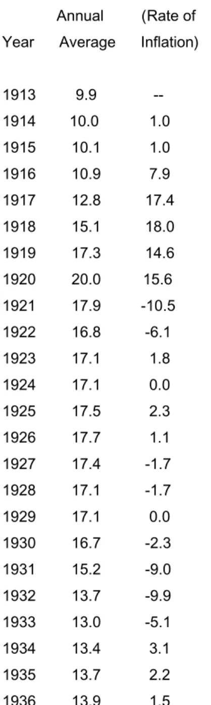
Table 2.5. CPI-U. [Ref: Consumer Price Index, 1913-2002.

CPI-U

Base year is chained; 1982-1984 = 100

Annual Percent Change Annual (Rate of Year Average Inflation) 1913 9.9 -- 1914 10.0 1.0 1915 10.1 1.0 1916 10.9 7.9 1917 12.8 17.4 1918 15.1 18.0 1919 17.3 14.6 1920 20.0 15.6 1921 17.9 -10.5 1922 16.8 -6.1 1923 17.1 1.8 1924 17.1 0.0 1925 17.5 2.3 1926 17.7 1.1 1927 17.4 -1.7 1928 17.1 -1.7 1929 17.1 0.0 1930 16.7 -2.3 1931 15.2 -9.0 1932 13.7 -9.9 1933 13.0 -5.1 1934 13.4 3.1 1935 13.7 2.2 1936 13.9 1.5

(33)

1937 14.4 3.6 1938 14.1 -2.1 1939 13.9 -1.4 1940 14.0 0.7 1941 14.7 5.0 1942 16.3 10.9 1943 17.3 6.1 1944 17.6 1.7 1945 18.0 2.3 1946 19.5 8.3 1947 22.3 14.4 1948 24.1 8.1 1949 23.8 -1.2 1950 24.1 1.3 1951 26.0 7.9 1952 26.5 1.9 1953 26.7 0.8 1954 26.9 0.7 1955 26.8 -0.4 1956 27.2 1.5 1957 28.1 3.3 1958 28.9 2.8 1959 29.1 0.7 1960 29.6 1.7 1961 29.9 1.0 1962 30.2 1.0 1963 30.6 1.3 1964 31.0 1.3 1965 31.5 1.6 1966 32.4 2.9 1967 33.4 3.1 1968 34.8 4.2 1969 36.7 5.5 1970 38.8 5.7 1971 40.5 4.4 1972 41.8 3.2

(34)

1973 44.4 6.2 1974 49.3 11.0 1975 53.8 9.1 1976 56.9 5.8 1977 60.6 6.5 1978 65.2 7.6 1979 72.6 11.3 1980 82.4 13.5 1981 90.9 10.3 1982 96.5 6.2 1983 99.6 3.2 1984 103.9 4.3 1985 107.6 3.6 1986 109.6 1.9 1987 113.6 3.6 1988 118.3 4.1 1989 124.0 4.8 1990 130.7 5.4 1991 136.2 4.2 1992 140.3 3.0 1993 144.5 3.0 1994 148.2 2.6 1995 152.4 2.8 1996 156.9 2.9 1997 160.5 2.3 1998 163.0 1.6 1999 166.6 2.2 2000 172.2 3.4 2001 177.1 2.8 2002 179.3* 1.2

*An estimate for 2002 is based on the change in the CPI from first quarter 2001 to first quarter 2002.

(35)

(36)

III. THE EFFECTS OF STATE INCOME TAXES ON THE

ELASTICITY OF INCOME

A. BACKGROUND AND GRAPHIC ILLUSTRATION OF DEADWEIGHT LOSS Martin Feldstein, Harvard University professor of economics and president of the National Bureau of Economic Research, used the Social Security tax to calculate the deadweight loss of the Social Security program. This chapter uses Feldstein’s methods and formulas—substituting California state income taxes for Social Security taxes—to calculate the deadweight loss and show how much greater it is when state taxes are imposed in addition to federal taxes on wages. The calculations for deadweight loss normally start with a zero tax base and add a tax to calculate deadweight loss.

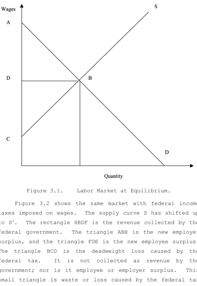
Figure 3.1 illustrates a labor market at equilibrium, without federal income taxes. The employer surplus is the area below the demand curve down to the wage paid and out to the quantity of labor supplied (triangle ABD). The employee surplus is the area above the supply curve up to the wage paid and out to the quantity of labor supplied (triangle DBC). No deadweight loss is incurred.

(37)

S D Wages Quantity B A C D S D Wages Quantity B A C D

Figure 3.1. Labor Market at Equilibrium.

Figure 3.2 shows the same market with federal income taxes imposed on wages. The supply curve S has shifted up to S1. The rectangle HBDF is the revenue collected by the federal government. The triangle ABH is the new employer surplus, and the triangle FDE is the new employee surplus. The triangle BCD is the deadweight loss caused by the federal tax. It is not collected as revenue by the government; nor is it employee or employer surplus. This small triangle is waste or loss caused by the federal tax on income.

(38)

H _B D F C D S S1_{(with FIT)} Wages Quantity G A E H _B D F C D S S1_{(with FIT)} Wages Quantity G A E

Figure 3.2. Labor Market with FIT.

Figure 3.3 illustrates the effect of imposing a state income tax in addition to a federal tax on wages. The total deadweight loss, represented by triangle BDF, is much larger. Deadweight loss caused by the state income tax is the trapezoid BCEF. The state revenue collected is the rectangle LBMJ. The federal revenue collected was the rectangle KCEI and is now the much smaller rectangle JMFH. Employer and employee surpluses are even smaller—i.e., the triangles ABL and HFG, respectively. The state income tax has exacerbated the deadweight loss from a federal tax on

(39)

wages. Once again, this much larger triangle, BDF, is revenue neither collected by the state or federal governments nor a gain to employee and employer surpluses.

K C E I D D S S1_{(with FIT)} Wages Quantity J A G B F H L M

S11_{(with FIT and SIT)}

N K C E I D D S S1_{(with FIT)} Wages Quantity J A G B F H L M

S11_{(with FIT and SIT)}

N

Figure 3.3. Labor Market with FIT and SIT. B. CALCULATING DEADWEIGHT LOSS (DWL)

Graphs are a simple way to visually demonstrate how taxes create deadweight loss. The next step is to quantify the DWL by using the same equation Feldstein used to calculate the DWL caused by a Social Security tax. Feldstein borrowed the equation, written in 1964 by

(40)

economist Arnold Harberger and modified by economist Edgar Browning in a piece written for the American Economic

Review titled, “On the Marginal Welfare Cost of Taxation.”

Feldstein explains how and why Browning modified the original equation for deadweight loss:

Browning (1987) showed that, when the relevant behavioral elasticity is measured in the presence of the tax, the original Hargberger (1964) formula for the deadweight loss of a tax with marginal tax rate t on a wage base of wL must be modified to DWL=0.5 ε t2_{wL/(1-t) where}_ε_{is the}

compensated elasticity of the tax base (wL) with respect to the marginal net of tax share, 1-t. The increase in the deadweight loss because the marginal tax rate is at t2 rather than t1 is

therefore ∆ DWL= 0.5 ε (t22 – t12)wL/ (1-t2). [Ref.

6:p. 9]

In the following tables, the modified formula DWL=0.5 ε t2 wL/(1-t) was used to calculate the deadweight loss from a state income tax on wages in 1958 and 1977. The 1958 dollar figures are inflation adjusted to 1977 dollars to facilitate comparison of same-year dollars. The calculations for ∆ DWL were accomplished by calculating the DWL in 1958, inflation adjusting to 1977 dollars and then subtracting that DWL from 1977's DWL, as opposed to using the equation above—i.e., ∆ DWL= 0.5 ε (t22 – t12)wL/(1-t2).

The purpose of the tables is to show how bracket creep exacerbates DWL from taxation.

Table 3.1, the first of four tables, uses an elasticity of .3. As will be demonstrated, DWL increases as elasticity increases.

(41)

wL58 58TR wL77 77TR Hr/yr E FIT t1 t1^2 t2 t2^2 1-t1 1-t2 adj dwl58 dwl77 adj Rev t1 Rev t2 D Rev D dwl Ddwl/Drev 1,000 $ 1% $ 2,097 1% 2000 0.3 15% 16% 2.56% 16% 2.560% 84% 84% $ 9.59 $ 9.59 $ 336 335.50 - $ - 0.00% 3,000 $ 1% $ 6,291 2% 2000 0.3 15% 16% 2.56% 17% 2.890% 84% 83% $ 28.76 $ 32.86 $ 1,007 1,069.41 62.91 $ 4.10 6.51% 4,000 $ 1% $ 8,388 3% 2000 0.3 15% 16% 2.56% 18% 3.240% 84% 82% $ 38.34 $ 49.71 $ 1,342 1,509.76 167.75 $ 11.37 6.78% 5,000 $ 1% $ 10,484 4% 2000 0.3 15% 16% 2.56% 19% 3.610% 84% 81% $ 47.93 $ 70.09 $ 1,678 1,992.04 314.53 $ 22.16 7.05% 7,000 $ 1% $ 14,678 5% 2000 0.3 15% 16% 2.56% 20% 4.000% 84% 80% $ 67.10 $ 110.09 $ 2,349 2,935.64 587.13 $ 42.99 7.32% 9,000 $ 1% $ 18,872 6% 2000 0.3 15% 16% 2.56% 21% 4.410% 84% 79% $ 86.27 $ 158.02 $ 3,020 3,963.11 943.60 $ 71.75 7.60% 10,000 $ 1% $ 20,969 7% 2000 0.3 15% 16% 2.56% 22% 4.840% 84% 78% $ 95.86 $ 195.17 $ 3,355 4,613.15 1,258.13 $ 99.31 7.89% 12,000 $ 2% $ 25,163 8% 2000 0.3 15% 17% 2.89% 23% 5.290% 83% 77% $ 131.42 $ 259.31 $ 4,278 5,787.40 1,509.76 $ 127.88 8.47% 13,000 $ 2% $ 27,260 9% 2000 0.3 15% 17% 2.89% 24% 5.760% 83% 76% $ 142.37 $ 309.90 $ 4,634 6,542.28 1,908.17 $ 167.52 8.78% 14,000 $ 2% $ 29,356 10% 2000 0.3 15% 17% 2.89% 25% 6.250% 83% 75% $ 153.33 $ 366.96 $ 4,991 7,339.10 2,348.51 $ 213.63 9.10% 15,000 $ 2% $ 31,453 11% 2000 0.3 15% 17% 2.89% 26% 6.760% 83% 74% $ 164.28 $ 431.00 $ 5,347 8,177.85 2,830.80 $ 266.72 9.42% 17,000 $ 2% $ 35,647 11% 2000 0.3 15% 17% 2.89% 26% 6.760% 83% 74% $ 186.18 $ 488.46 $ 6,060 9,268.24 3,208.24 $ 302.28 9.42% 20,000 $ 2% $ 41,938 11% 2000 0.3 15% 17% 2.89% 26% 6.760% 83% 74% $ 219.04 $ 574.66 $ 7,129 10,903.81 3,774.39 $ 355.62 9.42% 22,000 $ 3% $ 46,131 11% 2000 0.3 15% 18% 3.24% 26% 6.760% 82% 74% $ 273.41 $ 632.13 $ 8,304 11,994.19 3,690.52 $ 358.71 9.72% 25,000 $ 3% $ 52,422 11% 2000 0.3 15% 18% 3.24% 26% 6.760% 82% 74% $ 310.70 $ 718.33 $ 9,436 13,629.76 4,193.77 $ 407.63 9.72% 35,000 $ 4% $ 73,391 11% 2000 0.3 15% 19% 3.61% 26% 6.760% 81% 74% $ 490.63 $ 1,005.66 $ 13,944 19,081.66 5,137.37 $ 515.02 10.03% 45,000 $ 5% $ 94,360 11% 2000 0.3 15% 20% 4.00% 26% 6.760% 80% 74% $ 707.70 $ 1,292.99 $ 18,872 24,533.56 5,661.59 $ 585.29 10.34% 55,000 $ 6% $ 115,329 11% 2000 0.3 15% 21% 4.41% 26% 6.760% 79% 74% $ 965.70 $ 1,580.32 $ 24,219 29,985.47 5,766.44 $ 614.62 10.66%

Table 3.1. Deadweight Loss from State Taxes with an Elasticity of .3.

Refer to Table 3.1. Throughout all the analysis we assume, for computational simplicity, that the marginal tax rate is also the average tax rate on taxable income. In other words, we assume a flat tax rate. A married person filing a joint return in 1958 with a taxable income of $15,000 is in a marginal state income tax (SIT) bracket of two percent. Therefore, two percent of the person's incremental income is collected for SIT. This person pays a marginal federal income tax rate (FIT) of 15 percent; thus, his combined total tax rate, SIT + FIT, is 17 percent. Assuming that he does not receive any real pay increases, after adjusting for inflation he earns $31,453 in 1977 dollars and is now paying an 11 percent SIT. The percentage increase in his marginal tax rate is 450%. The DWL for 1958 and inflation-adjusted to 1977 is $164.28. The DWL for 1977 is $431 and the delta, or increase in DWL from 1958 to 1977, is $266.72. The revenue collected in 1958 and adjusted for inflation to 1977 is $5,347. Revenue for 1977 is $8,177. The delta, or increase in revenue from 1958 to 1977, is $2831. By dividing the delta DWL by the

(42)

delta revenue, the DWL as percentage of revenue collected is calculated at 9.42 percent. This means that it costs 9.42 cents for every additional dollar collected in revenue from this person, or that 9.42 cents on the dollar is lost to DWL. Notice that for a person in the highest marginal SIT bracket for 1977, 11 percent, it costs more than ten cents for every dollar collected as revenue.

Table 3.2 is the same as Table 3.1 with the exception of elasticity. If elasticity is increased to .5, the incremental DWL as percentage of incremental revenue collected is now 15.70 percent and almost 18 percent for the highest marginal tax bracket. And for Tables 3.3 and 3.4, the incremental DWL as percentage of incremental revenue collected for the person earning $15,000 in 1958 and for a person in the highest marginal tax bracket are 21.98/31.41 and 24.87/35.53 percent, respectively.

wL58 58TR wL77 77TR Hr/yr E FIT t1 t1^2 t2 t2^2 1-t1 1-t2 adj dwl58 dwl77 adj Rev t1 Rev t2 D Rev D dwl Ddwl/Drev 1,000 $ 1% $ 2,097 1% 2000 0.5 15% 16% 2.56% 16% 2.560% 84% 84%$ 15.98 $ 15.98 $ 335.50 $ 335.50 $ - $ - 0.00% 3,000 $ 1% $ 6,291 2% 2000 0.5 15% 16% 2.56% 17% 2.890% 84% 83%$ 47.93 $ 54.76 $ 1,006.51 $ 1,069.41 $ 62.91 $ 6.83 10.86% 4,000 $ 1% $ 8,388 3% 2000 0.5 15% 16% 2.56% 18% 3.240% 84% 82%$ 63.91 $ 82.85 $ 1,342.01 $ 1,509.76 $ 167.75 $ 18.95 11.30% 5,000 $ 1% $ 10,484 4% 2000 0.5 15% 16% 2.56% 19% 3.610% 84% 81%$ 79.88 $ 116.82 $ 1,677.51 $ 1,992.04 $ 314.53 $ 36.94 11.74% 7,000 $ 1% $ 14,678 5% 2000 0.5 15% 16% 2.56% 20% 4.000% 84% 80%$ 111.83 $ 183.48 $ 2,348.51 $ 2,935.64 $ 587.13 $ 71.64 12.20% 9,000 $ 1% $ 18,872 6% 2000 0.5 15% 16% 2.56% 21% 4.410% 84% 79%$ 143.79 $ 263.37 $ 3,019.52 $ 3,963.11 $ 943.60 $ 119.59 12.67% 10,000 $ 1% $ 20,969 7% 2000 0.5 15% 16% 2.56% 22% 4.840% 84% 78%$ 159.76 $ 325.29 $ 3,355.02 $ 4,613.15 $ 1,258.13 $ 165.52 13.16% 12,000 $ 2% $ 25,163 8% 2000 0.5 15% 17% 2.89% 23% 5.290% 83% 77%$ 219.04 $ 432.18 $ 4,277.65 $ 5,787.40 $ 1,509.76 $ 213.14 14.12% 13,000 $ 2% $ 27,260 9% 2000 0.5 15% 17% 2.89% 24% 5.760% 83% 76%$ 237.29 $ 516.50 $ 4,634.12 $ 6,542.28 $ 1,908.17 $ 279.21 14.63% 14,000 $ 2% $ 29,356 10% 2000 0.5 15% 17% 2.89% 25% 6.250% 83% 75%$ 255.54 $ 611.59 $ 4,990.59 $ 7,339.10 $ 2,348.51 $ 356.05 15.16% 15,000 $ 2% $ 31,453 11% 2000 0.5 15% 17% 2.89% 26% 6.760% 83% 74%$ 273.80 $ 718.33 $ 5,347.06 $ 8,177.85 $ 2,830.80 $ 444.53 15.70% 17,000 $ 2% $ 35,647 11% 2000 0.5 15% 17% 2.89% 26% 6.760% 83% 74%$ 310.30 $ 814.10 $ 6,060.00 $ 9,268.24 $ 3,208.24 $ 503.80 15.70% 20,000 $ 2% $ 41,938 11% 2000 0.5 15% 17% 2.89% 26% 6.760% 83% 74%$ 365.06 $ 957.77 $ 7,129.41 $ 10,903.81 $ 3,774.39 $ 592.71 15.70% 22,000 $ 3% $ 46,131 11% 2000 0.5 15% 18% 3.24% 26% 6.760% 82% 74%$ 455.69 $ 1,053.54 $ 8,303.67 $ 11,994.19 $ 3,690.52 $ 597.85 16.20% 25,000 $ 3% $ 52,422 11% 2000 0.5 15% 18% 3.24% 26% 6.760% 82% 74%$ 517.83 $ 1,197.21 $ 9,435.99 $ 13,629.76 $ 4,193.77 $ 679.38 16.20% 35,000 $ 4% $ 73,391 11% 2000 0.5 15% 19% 3.61% 26% 6.760% 81% 74%$ 817.72 $ 1,676.09 $ 13,944.29 $ 19,081.66 $ 5,137.37 $ 858.37 16.71% 45,000 $ 5% $ 94,360 11% 2000 0.5 15% 20% 4.00% 26% 6.760% 80% 74%$ 1,179.50 $ 2,154.98 $ 18,871.97 $ 24,533.56 $ 5,661.59 $ 975.48 17.23% 55,000 $ 6% $ 115,329 11% 2000 0.5 15% 21% 4.41% 26% 6.760% 79% 74%$ 1,609.49 $ 2,633.86 $ 24,219.03 $ 29,985.47 $ 5,766.44 $ 1,024.37 17.76%

(43)

wL58 58TR wL77 77TR Hr/yr E FIT t1 t1^2 t2 t2^2 1-t1 1-t2 dwl58 dwl77 Rev t1 Rev t2 D Rev D dwl Ddwl/Drev 1,000 $ 1% $ 2,097 1% 2000 0.7 15% 16% 2.56% 16% 2.560% 84% 84%$ 22.37 $ 22.37 $ 335.50 $ 335.50 $ - $ - 0.00% 3,000 $ 1% $ 6,291 2% 2000 0.7 15% 16% 2.56% 17% 2.890% 84% 83%$ 67.10 $ 76.66 $ 1,006.51 $ 1,069.41 $ 62.91 $ 9.56 15.20% 4,000 $ 1% $ 8,388 3% 2000 0.7 15% 16% 2.56% 18% 3.240% 84% 82%$ 89.47 $ 115.99 $ 1,342.01 $ 1,509.76 $ 167.75 $ 26.53 15.81% 5,000 $ 1% $ 10,484 4% 2000 0.7 15% 16% 2.56% 19% 3.610% 84% 81%$ 111.83 $ 163.54 $ 1,677.51 $ 1,992.04 $ 314.53 $ 51.71 16.44% 7,000 $ 1% $ 14,678 5% 2000 0.7 15% 16% 2.56% 20% 4.000% 84% 80%$ 156.57 $ 256.87 $ 2,348.51 $ 2,935.64 $ 587.13 $ 100.30 17.08% 9,000 $ 1% $ 18,872 6% 2000 0.7 15% 16% 2.56% 21% 4.410% 84% 79%$ 201.30 $ 368.72 $ 3,019.52 $ 3,963.11 $ 943.60 $ 167.42 17.74% 10,000 $ 1% $ 20,969 7% 2000 0.7 15% 16% 2.56% 22% 4.840% 84% 78%$ 223.67 $ 455.40 $ 3,355.02 $ 4,613.15 $ 1,258.13 $ 231.73 18.42% 12,000 $ 2% $ 25,163 8% 2000 0.7 15% 17% 2.89% 23% 5.290% 83% 77%$ 306.65 $ 605.05 $ 4,277.65 $ 5,787.40 $ 1,509.76 $ 298.40 19.76% 13,000 $ 2% $ 27,260 9% 2000 0.7 15% 17% 2.89% 24% 5.760% 83% 76%$ 332.20 $ 723.09 $ 4,634.12 $ 6,542.28 $ 1,908.17 $ 390.89 20.49% 14,000 $ 2% $ 29,356 10% 2000 0.7 15% 17% 2.89% 25% 6.250% 83% 75%$ 357.76 $ 856.23 $ 4,990.59 $ 7,339.10 $ 2,348.51 $ 498.47 21.22% 15,000 $ 2% $ 31,453 11% 2000 0.7 15% 17% 2.89% 26% 6.760% 83% 74%$ 383.31 $ 1,005.66 $ 5,347.06 $ 8,177.85 $ 2,830.80 $ 622.34 21.98% 17,000 $ 2% $ 35,647 11% 2000 0.7 15% 17% 2.89% 26% 6.760% 83% 74%$ 434.42 $ 1,139.74 $ 6,060.00 $ 9,268.24 $ 3,208.24 $ 705.32 21.98% 20,000 $ 2% $ 41,938 11% 2000 0.7 15% 17% 2.89% 26% 6.760% 83% 74%$ 511.08 $ 1,340.87 $ 7,129.41 $ 10,903.81 $ 3,774.39 $ 829.79 21.98% 22,000 $ 3% $ 46,131 11% 2000 0.7 15% 18% 3.24% 26% 6.760% 82% 74%$ 637.96 $ 1,474.96 $ 8,303.67 $ 11,994.19 $ 3,690.52 $ 837.00 22.68% 25,000 $ 3% $ 52,422 11% 2000 0.7 15% 18% 3.24% 26% 6.760% 82% 74%$ 724.96 $ 1,676.09 $ 9,435.99 $ 13,629.76 $ 4,193.77 $ 951.13 22.68% 35,000 $ 4% $ 73,391 11% 2000 0.7 15% 19% 3.61% 26% 6.760% 81% 74%$ 1,144.81 $ 2,346.53 $ 13,944.29 $ 19,081.66 $ 5,137.37 $ 1,201.72 23.39% 45,000 $ 5% $ 94,360 11% 2000 0.7 15% 20% 4.00% 26% 6.760% 80% 74%$ 1,651.30 $ 3,016.97 $ 18,871.97 $ 24,533.56 $ 5,661.59 $ 1,365.67 24.12% 55,000 $ 6% $ 115,329 11% 2000 0.7 15% 21% 4.41% 26% 6.760% 79% 74%$ 2,253.29 $ 3,687.40 $ 24,219.03 $ 29,985.47 $ 5,766.44 $ 1,434.11 24.87%

wL58 58TR wL77 77TR Hr/yr E FIT t1 t1^2 t2 t2^2 1-t1 1-t2 adj dwl58 dwl77 adj Rev t1 Rev t2 D Rev D dwl Ddwl/Drev

1,000 $ 1% $ 2,097 1% 2000 1 15% 16% 2.56% 16% 2.560% 84% 84% $ 31.95 $ 31.95 $ 336 335.50 - $ - 0.00% 3,000 $ 1% $ 6,291 2% 2000 1 15% 16% 2.56% 17% 2.890% 84% 83% $ 95.86 $ 109.52 $ 1,007 1,069.41 62.91 $ 13.66 21.72% 4,000 $ 1% $ 8,388 3% 2000 1 15% 16% 2.56% 18% 3.240% 84% 82% $ 127.81 $ 165.71 $ 1,342 1,509.76 167.75 $ 37.89 22.59% 5,000 $ 1% $ 10,484 4% 2000 1 15% 16% 2.56% 19% 3.610% 84% 81% $ 159.76 $ 233.63 $ 1,678 1,992.04 314.53 $ 73.87 23.49% 7,000 $ 1% $ 14,678 5% 2000 1 15% 16% 2.56% 20% 4.000% 84% 80% $ 223.67 $ 366.96 $ 2,349 2,935.64 587.13 $ 143.29 24.40% 9,000 $ 1% $ 18,872 6% 2000 1 15% 16% 2.56% 21% 4.410% 84% 79% $ 287.57 $ 526.74 $ 3,020 3,963.11 943.60 $ 239.17 25.35% 10,000 $ 1% $ 20,969 7% 2000 1 15% 16% 2.56% 22% 4.840% 84% 78% $ 319.53 $ 650.57 $ 3,355 4,613.15 1,258.13 $ 331.05 26.31% 12,000 $ 2% $ 25,163 8% 2000 1 15% 17% 2.89% 23% 5.290% 83% 77% $ 438.07 $ 864.35 $ 4,278 5,787.40 1,509.76 $ 426.28 28.24% 13,000 $ 2% $ 27,260 9% 2000 1 15% 17% 2.89% 24% 5.760% 83% 76% $ 474.58 $ 1,032.99 $ 4,634 6,542.28 1,908.17 $ 558.41 29.26% 14,000 $ 2% $ 29,356 10% 2000 1 15% 17% 2.89% 25% 6.250% 83% 75% $ 511.08 $ 1,223.18 $ 4,991 7,339.10 2,348.51 $ 712.10 30.32% 15,000 $ 2% $ 31,453 11% 2000 1 15% 17% 2.89% 26% 6.760% 83% 74% $ 547.59 $ 1,436.65 $ 5,347 8,177.85 2,830.80 $ 889.06 31.41% 17,000 $ 2% $ 35,647 11% 2000 1 15% 17% 2.89% 26% 6.760% 83% 74% $ 620.60 $ 1,628.20 $ 6,060 9,268.24 3,208.24 $ 1,007.60 31.41% 20,000 $ 2% $ 41,938 11% 2000 1 15% 17% 2.89% 26% 6.760% 83% 74% $ 730.12 $ 1,915.53 $ 7,129 10,903.81 3,774.39 $ 1,185.41 31.41% 22,000 $ 3% $ 46,131 11% 2000 1 15% 18% 3.24% 26% 6.760% 82% 74% $ 911.38 $ 2,107.09 $ 8,304 11,994.19 3,690.52 $ 1,195.71 32.40% 25,000 $ 3% $ 52,422 11% 2000 1 15% 18% 3.24% 26% 6.760% 82% 74% $ 1,035.66 $ 2,394.42 $ 9,436 13,629.76 4,193.77 $ 1,358.76 32.40% 35,000 $ 4% $ 73,391 11% 2000 1 15% 19% 3.61% 26% 6.760% 81% 74% $ 1,635.44 $ 3,352.18 $ 13,944 19,081.66 5,137.37 $ 1,716.74 33.42% 45,000 $ 5% $ 94,360 11% 2000 1 15% 20% 4.00% 26% 6.760% 80% 74% $ 2,359.00 $ 4,309.95 $ 18,872 24,533.56 5,661.59 $ 1,950.95 34.46% 55,000 $ 6% $ 115,329 11% 2000 1 15% 21% 4.41% 26% 6.760% 79% 74% $ 3,218.99 $ 5,267.72 $ 24,219 29,985.47 5,766.44 $ 2,048.73 35.53%

Table 3.4. Deadweight Loss from State Taxes with an Elasticity of 1.

The worst-case scenario, or the scenario that creates the most extra waste as a percentage of extra revenue collected, is for a person in the highest marginal tax bracket with an elasticity of 1. It costs more than one dollar to collect three dollars in revenue from this person. One out of every three dollars is wasted.

(44)

IV. CONCLUSION

A. CONCLUSIONS

One of the major factors in the location of economic activity is the tax system in that location. All other things equal, the lower the tax rate in an area, the more attractive the area is for economic activity. This matters for location across states, because movement from one state to another is relatively low cost. The fact that workers can move from California to Nevada, for example, means that wages net of taxes will tend to equalize, which means that wages net of taxes will tend to be higher in the high-tax-rate state. This fact, in turn, means that production will be more expensive in the high-tax state. This is particularly relevant for defense production and even location of military bases, because the Department of Defense (DoD) often has the option of choosing one state over another.

Bracket creep, if left unchecked, will cause deadweight to continue to grow. It is unrealistic to expect state taxes to go away entirely. But deadweight loss incurred by over-taxation due to bracket creep can be minimized. Industries, especially defense related industries, do have options for locating plants, companies and other defense related service. The amount of taxes Californians pay due to bracket creep affects the wage levels of employees. Defense industries looking for a future location, or deciding whether or not to remain in California must take wages--and therefore state income tax rates--into consideration when making those decisions.

(45)

(46)

LIST OF REFERENCES

1. State of California Technology, Trade & Commerce Agency 16 Oct 2001.

<commerce.ca.gov/state/ttca/ttca_homepage.jsp>. 2. James E. Hartley, Steven M. Sheffrin and J. David

Vasche, “Reform During Crisis: The Transformation of California’s Fiscal System During the Great

Depression,” Journal of Economic History 56.3 (1996). 3. David R. Doerr, “Capsule History of the California Tax

Structure: Part IV, Chapter One – The Tax and Spend Years, 1933-1958,” Cal-Tax Digest November (1997). 4. David R. Doerr, “Capsule History of the California Tax

Structure: Part IV, Chapter Two – The Tax and Spend Years, 1959-1967,” Cal-Tax Digest December (1997). 5. Taxopedia,

http://www.taxopedia.com/terms/b/bracketcreep.asp. 6. Martin Feldstein, “The Missing Piece in Policy

Analysis: Social Security Reform," American Economic

Review, Vol. 86, No. 2 (May 1996).

7. Edgar K. Browning, “On the Marginal Welfare Cost of Taxation,” American Economic Review, Vol. 77, Issue 1 (Mar 1987), 11-23.

(47)

(48)