Expertise-based decision makers’ importance weights for
solving group decision making problems under fuzzy
preference relations
E Herowati
Department of Industrial Engineering, University of Surabaya, Raya Kalirungkut, Surabaya, 60293, Indonesia
Abstract. The quality of a decision is influenced by the level of expertise of the Decision Makers (DMs). In Group Decision Making, alternatives’ scores are obtained by integrating the DMs opinions and the importance weights of the DMs greatly affect the resulted value. Expertise level is defined as the ability to differentiate consistently and expressed as the CWS-Index, a ratio between the Discrimination and Inconsistency. The DMs give their evaluations in pairwise comparison of Fuzzy Preference Relations (FPR) and the additivity property of FPR generates the estimators needed to get the CWS-Indexes and the expertise-based ranking of DMs. The weights of the DMs are obtained by using Induced Ordered Weighted Averaging (IOWA) operator and Basic Unit Monotonic Increasing functions and the resulted weights are used to evaluate the available alternatives to get the best one based on Fuzzy Majority and IOWA operators. This paper proposed an expertise-based weight allocation method for DMs and a numerical example is discussed to illustrate this expertise-based model to get the best alternative and it concluded that the higher the DMs’ expertise level, the higher his/her weight, and these weights affect the alternatives’ score and the rank of the alternatives.
1. Introduction
Experts have the ability to think differently and this ability underlies the high quality of their decision making [1]. In Group Decision Making (GDM), a group of Decision Makers (DMs) with different expertise, interest and background have to evaluate several alternatives to be chosen in a selection process. The value of each alternative is obtained from group assessment that synthesizes all the DMs’ individual values by aggregating their values mathematically [2]. Since the DMs have different expertise, knowledge and background, their individual values should be aggregated by using different importance weights. Assigning inappropriate importance weights of DMs can lead to incorrect results in obtaining the final selection [3],
therefore
researches related to GDM and DMs’ Importance weight are increasingly developing [4] .Researches related to the DMs’ importance weight have been carried out previously. In the beginning, the DMs’ importance weight were determined subjectively based on people's views on the DMs, for example an influential person determining the DMS weight directly [5] and a group of assessors who were considered experts assessing the DMs to obtain their importance weights [6] The subjectivity and difficulty of the assessors to evaluate DMs correctly has the potential to lead to biased decisions.
The DMs' importance weight can be determined objectively by observing the results of their assessment on a set of alternatives. The DMs' weight can be determined based on group consensus [7], in the sense that DM whose opinion increases consensus is given a larger weight. In addition, DM who assigned larger weight is the DM with a smaller deviation or smaller distance [8] from group composite value. The consistency of DM evaluations towards alternatives was also used to determine the weight of the related DM in several researches [9]. The DMS’ weights that are obtained objectively are considered better than the DMs’ weights that are determined subjectively, but there are still some decision biases that need to be considered, for example opinion that are approved by most people are not necessarily the right opinion and all of the above studies have not considered the expertise level of the DMs where the more expert a DM is the better the quality of the decision will be. There are several researches related to expertise level, for example expertise-based DM ranking [10-12] and expertise-based DMs’ importance weights [13]. In these studies, DMs assessed the alternatives in the form of Fuzzy Preference Relations (FPR) and the DMs’ weights obtained are objective and based on their expertise but these weights should be revised since those researches have not considered reciprocal relations of FPR since an expert can certainly compare the value of two alternatives smartly. If he judges the first alternative is better than the second alternative by some degree, then the reciprocal relation ensures that there is no need for him to re-evaluate by comparing the second alternative to the first one. This study proposes the revised version of expertise-based DMs’ importance weights considering reciprocal relations and illustrated by examples used in prior expertise-based researches.
2. Literature reviews
2.1.Expertise level of the decision makers
An expert in a particular field is someone who has a strong background in this field. Shanteau et al [14] defines expertise as the ability to differentiate consistently, expressed as CWS-Index as shown in (1).
CWS‐Index
DiscriminationInconsistensy variance of the same alternativevariance of different alternatives’’s values values 1 ) ( 2 1
n GM M r n j j ) 1 ( ) ( 1 2 1
r n M M n j j ij r i(1)
Where: r : The number of replications j
M
: The average of individual values for case-j GM : The grand mean of all individual valuesn : The number of different cases ij
M
: The individual value for replication-i case-jThe evaluated DMs must repeat their assessment to obtain a measure of inconsistency.
2.2.The FPR and additive consistency property
Chiclana et al [15] proposed GDM model where a group of m experts E{e1,e2,...em}, m2
evaluate a set of n alternatives X {x1,x2,...xn}, n2 in FPR P XxX having a membership function
] 1 , 0 [ :XxX p
and represented by means of the n x n matrix
P
(
p
ij)
. pijis the preference degreeof
x
ioverx
j. 12 ijThe FPR P has a reciprocal relation as shown in (2) and the matrix P as shown in (3). Additive Consistency (AC) property of FPR among three alternatives
x
i,x
j,x
k( , , 1,2, . . . , ) yields 3formulas ( , g=1,2,3) to estimate
p
ik as in (4), (5) and (6).1 ji ij p p (2) 5 . 0 1 1 1 5 . 0 1 1 5 . 0 1 5 . 0 34 24 14 34 23 13 24 23 12 14 13 12 p p p p p p p p p p p p P (3) 2 1 1 jk ij j ik p p p ,ji,k (4) 2 1 2 ji jk j ik p p p , ji,k (5) 2 1 3 kj ij j ik p p p ,ji,k (6)
For every element of the matrix FPR pij, there are 3x(n-2) replications (3 formulas and
j
i
,
k
)and has the range of [-0.5, 1.5]. If the reciprocal relation is considered, the 3 formulas are just one formula and the number of replications is reduced to (n-2). To keep the range of estimated value of
p
ikbetween [0,1], all of the elementp
ikshould be transformed usinga a x x f 2 1 ) (
and the range changes from [a, 1a] ,
0
a to [0,1][15].
2.3.The induced OWA operator
Yager [16] proposed an n-dimensional OWA Operator F:InI where
n j j j n w a a a w b F 1 2 1, ,..., ) ( , j bis the jth largest element of input arguments (a1,a2,...,an), wj is the ordered weight, and wj0, 1
1
n
j wj .The Induced OWA Operator is an OWA Operator using the order inducing variable as the ordering of the input arguments. An n dimensional Induced OWA Operator F:In I where
n j j j n n w u a u a u a w b F 1 2 2 1 1, , , ,..., , ) (, ui is the order inducing variable, ai is the input argument, j
w is the order weights and wj 0, 1 1
n j wj , j bis the input argument with the j-th largest the order inducing variable value. The OWA weights can be obtained by using Basic Unit Monotonic Function (BUM) Q:[0,1][0,1], Q(0)0;Q(1)1;Q(x)Q(y) if x y as follows [16]:
1 j j j QR QR w (7) where Rj> Rj1,wj0, 1 1
n j jw . The accumulative value of the DMs’ weights is associated with the BUM as in Figure 1, hence the DMs weights will never negative (wj0) with the total weights are
one.
2.4.Quantifier guided dominance degree
Quantifier Guided Dominance Degree (QGDD) quantify the dominance of alternative- over all of the others in a fuzzy majority as in (8).
, 1,2, … , (8)
The ranking of alternatives are determined based on ranking of their QGDD.
Figure 1. The OWA Weights from BUM
3. The proposed method
The steps used to select alternatives proposed in this study are as follows:
1) Combine shanteau‘s expertise level and the AC property of FPR. The DMs’ assessment must be given in FPR and we don’t need repetition to measure consistency in expertise, and we get the CWS-Index for FPR in equation (9) and yield the CWS-Indexes and DMs’ rank [12].
CWS-Index Variance of different 'pairwise comparisons between two alternatives'
Variance of the same 'pairwise comparisons between two alternative's' (9) 2) Combine the ordered Indexes and BUM, the accumulated logarithmic ordered
CWS-Indexes are used as the horizontal axis of the BUM. Herowati et al [13] used BUM Q(R)=Rn, n ≤ 1 and this research revises the BUM to be a straight line, Q(R)=R to ensure that the DMs with the same expertise level will assigned the same weight and there are only (n-2) replications in this study instead of 3(n-2) in [13] since the previous study didn’t consider the reciprocal relation as in equation (2).
3) Aggregate the individual FPR of all DMs by using the weights generated from the previous step to form a FPR group and this value is used in the selection process using the concepts of QGDD.
4. Illustrative example
We provide a numerical example to illustrate the proposed method. Suppose 5 DMs
}
,
,
,
,
{
e
1e
2e
3e
4e
5E
assess a set of four alternativesX {x1,x2,x3,x4}in form of Matrix FPR P as follows: 50 . 0 30 . 0 30 . 0 60 . 0 70 . 0 50 . 0 60 . 0 60 . 0 70 . 0 40 . 0 50 . 0 60 . 0 40 . 0 40 . 0 40 . 0 50 . 0 1 P 50 . 0 55 . 0 40 . 0 55 . 0 45 . 0 50 . 0 35 . 0 60 . 0 60 . 0 65 . 0 50 . 0 70 . 0 45 . 0 40 . 0 30 . 0 50 . 0 2 P 50 . 0 40 . 0 60 . 0 30 . 0 60 . 0 50 . 0 70 . 0 40 . 0 40 . 0 30 . 0 50 . 0 10 . 0 70 . 0 60 . 0 90 . 0 50 . 0 3 P 50 . 0 90 . 0 65 . 0 30 . 0 10 . 0 50 . 0 40 . 0 20 . 0 35 . 0 60 . 0 50 . 0 60 . 0 70 . 0 80 . 0 40 . 0 50 . 0 4 P 50 . 0 60 . 0 45 . 0 40 . 0 40 . 0 50 . 0 35 . 0 20 . 0 55 . 0 65 . 0 50 . 0 30 . 0 60 . 0 80 . 0 70 . 0 50 . 0 5 P1) Estimate each element Matrix P4 by using one of the formula 1, 2 or 3 to generate 2 estimated value as shown in column 3 and 4 of Table 1. For each element there are 3 values (r=3), i.e. the original value and 2 estimated values. Transform the values outside the range of [0,1] by using transformation function 1 . 0 2 1 1 . 0 ) ( x x x f
as shown in column 5,6,7 of Table 1.
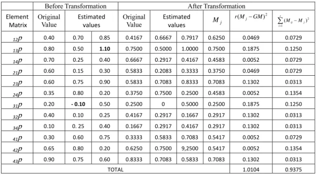
Discrimination= 1 ) ( 2 1 n GM M r n j j = 0.09186 ) 1 12 ( 1.01042 ;Inconsistency = ( 1) ) ( 1 2 1
r n M M n j j ij r i = 0.03906 ) 1 3 ( 12 0.93750 x CWS-Index for DM – 4 =00..0390609186 2.3518CWS-Indexes for DM-1, DM-2, DM-3, DM-4 and DM-5 subsequently are 3.8395, 22.039, 52.1267, 2.3518 and 18.757 and the DMs rank is DM-3, DM-2, DM-5, DM-1 and DM-4.
2) The rank of the DMs obtained in step 1) and the CWS-Indexes are ordered as in Table 2, then the ordered CWS-Indexes were transformed by using the logarithmic function and accumulated and normalized. The normalized(Accumulated(Log(CWS-Index))) is the horizontal axis of the straight line BUM and we get the DMs’ importance weights as in the last row of Table 2.
3) Aggregate the individual FPR of all DMs by using the importance weights to form a FPR group and calculate the QGDD by using fuzzy majority function ‘Most’ which has the weights to compare with the other three alternatives (1/15 , 10/15, 4/15).
500 , 0 510 , 0 483 , 0 421 , 0 490 , 0 500 , 0 495 , 0 411 , 0 517 , 0 505 , 0 500 , 0 391 , 0 579 . 0 589 , 0 609 , 0 500 , 0 Grup P
p12calculation to illustrate the aggregation process from individual FPRs to group FPR:
12
p
0,105x0,4 + 0,2539x0,3 + 0,3247x0,9 + 0,0702x0,6 + 0,2407x0,7 = 0,609The first row of the FPR group is the group value of the first alternative, the second row are the value for the second alternative. The QGDD for all the alternatives are calculated by using fuzzy majority ‘Most’ with the weight (1/15 , 10/15, 4/15) and the element matrix values have to be ordered before the calculation. For example QGDD for alternative-2 are as follows:
4755 , 0 391 , 0 505 , 0 517 , 0 ) 2 , ,..., 2 , 1 , ( 2 151 1510 154 2 F p j n j x x x QGDD q Grupj
Table 1. Example of CWS-Index calculation for DM-4
Before Transformation After Transformation
Element Matrix Original Value Estimated values Original Value Estimated values Mj 2 ) (M GM r j r i j ij M M 1 2 ) ( p 12 0.40 0.70 0.85 0.4167 0.6667 0.7917 0.6250 0.0469 0.0729 p 13 0.80 0.50 1.10 0.7500 0.5000 1.0000 0.7500 0.1875 0.1250 p 14 0.70 0.25 0.40 0.6667 0.2917 0.4167 0.4583 0.0052 0.0729 p 21 0.60 0.15 0.30 0.5833 0.2083 0.3333 0.3750 0.0469 0.0729 p 23 0.60 0.75 0.90 0.5833 0.7083 0.8333 0.7083 0.1302 0.0313 p 24 0.35 0.80 0.20 0.3750 0.7500 0.2500 0.4583 0.0052 0.1354 p 31 0.20 ‐ 0.10 0.50 0.2500 0 0.5000 0.2500 0.1875 0.1250 p 32 0.40 0.10 0.25 0.4167 0.2917 0.1667 0.2917 0.1302 0.0313 p 34 0.10 0. 25 0.40 0.1667 0.2917 0.4167 0.2917 0.1302 0.0313 p 41 0.30 0.60 0.75 0.3333 0.5833 0.7083 0.5417 0.0052 0.0729 p 42 0.65 0.80 0.20 0.6250 0.7500 9,2500 0.5417 0.0052 0.1354 p 43 0.90 0.75 0.60 0.8333 0.7083 0.5833 0.7083 0.1302 0.0313 TOTAL 1.0104 0.9375
Table 2. The DMs’ importance weights calculation
DM‐3 DM‐2 DM‐5 DM‐1 DM‐4 CWS- Index 52,1267 22,0390 18,7570 3,8395 2,3518 Log(CWS-Index) 1,7171 1,3432 1,2732 0,5843 0,3714 Accumulated(Log(CWS-Index)) 1,7171 3,0603 4,3334 4,9177 5,2891 R=Normalized(Accumulated(Log(CWS-Index))) 0,3246 0,5786 0,8193 0,9298 1,0000 R R R Q( ) 0,3246 0,5786 0,8193 0,9298 1,0000 DMs’ Importance Weights 0,3246 0,2539 0,2407 0,1105 0,0702
Table 3. Comparison of the results of the selection process
Expertise-based DMs’ weights (0,11, 0,25, 0,33, 0,07, 0,24)
DMs’ Average Weight (1/5 , 1/5, 1/5, 1/5 , 1/5, 1/5)
Inverse Expertise-based DMs’ weights (0,25, 0,11, 0,07, 0,33, 0,24)
QGDD Rank QGDD Rank QGDD Rank
Alternative -1 0,588 1 0,564 1 0,556 1
Alternative -3 0,469 3 0,439 4 0,392 4
Alternative -4 0,468 4 0,471 3 0,475 3
Table 3 shown that expertise-based DMs’ importance weights yields alternatives ranking 1, 2, 3, 4. If the aggregation process uses DMS’ average weights or for all the DMs, then the alternatives ranking are 1, 2, 4 and 3. The use of average as DMs' importance weights does not have any effect if we want to choose one best alternative. But if we want to eliminate one unwanted alternative, the results will be different from results based on expertise. The third case, inverse expertise-based uses of DMs' importance weights in reverse manner where the more expert a DM is, the smaller the weight and yield the same result with the second case. In this illustrative example, the expertise of the DMs are assumed to be unknown and not determined by the people's subjective view of these DMs. Expertise from DMS are determined based on their assessment of alternatives by using the Shanteau’s concept, experts are those who can distinguish alternatives consistently and expressed by the CWS Indexes and the integration of DMs opinion using expertise-based weights yield different rank of alternatives and it is expected to produce a better decisions
5. Conclusion
This paper revises expertise-based DMs' importance weights by considering reciprocal relations since it is more realistic when assessed DMs are carrying out their assessment task.The application of expertise -based DMs weights in this paper shows that DMs weights affects the alternatives’ score and the alternatives’ rank and it is expected that expertise-based DMs' weights leads to a better decisions.
Reference
[1] Malhotra V, Lee M D and Khurana A 2007 Domain experts influence decision quality: Towards a robust method for their identification J Pet Sci Eng 57 (1-2) pp 181–94
[2] Cooke R M 1991 Experts in uncertainty opinion and subjective probability in science (New York/Oxford: Oxford University Press)
[3] Emrah K and Kabak O 2019 Deriving decision makers’ weights in group decision making: An overview of objective methods Information Fusion 49 pp 146–60
[4] Kabak O and Ervural B 2017 Multiple attribute group decision making: a generic conceptual framework and a classification scheme Knowledge-Based System 123 pp 13–30
[5] Herrera F, Herrera-Viedma E and Verdegay J L 1998 Choice processes for non-homogeneous group decision making in linguistic setting Fuzzy Sets Syst. 94(3) pp 287–308
[6] Ramanathan R and Ganesh L S 1994 Group preference aggregation methods employed in AHP: An evaluation and an intrinsic process for deriving members' weightages Eur. J.
Oper. Res. 79(2) pp 249–65
[7] Kacprzyk J, Fedrizzi M and Nurmi H 1992 Group decision making and consensus under fuzzy preferences and fuzzy majority Fuzzy Sets Syst. 49 pp 21–31
[8] Chuan Y 2017 Entropy-based weights on decision makers in group decision making setting with hybrid preference representations Appl. Soft Comput 60 pp 737–49
[9] Alonso S, Cabrerizo F, Chiclana F, Herrera F and Herrera-Viedma E 2009 Group decision making with incomplete fuzzy linguistic preference relations Int. J. Intell. Syst. 24(2) pp 201–22
[10] Herowati E, Ciptomulyono U, Parung J and Suparno 2013 Competent-based experts’ ranking at fuzzy preference relations on alternatives. Proc. Int. Conf. on Industrial Engineering and
Service Science (Surabaya: Sepuluh Nopember Institute of Technology, Indonesia)
[11] Herowati E, Ciptomulyono U, Parung J, Suparno 2014 Expertise-based experts ranking at multiplicative preference relations on alternatives. Proc. Int. Conf. Asia Pacific Industrial
Engineering & Management Society (Jeju Island: South Korea)
[12] Herowati E, Ciptomulyono U, Parung J and Suparno 2017 Expertise-based ranking of experts: An assessment level approach Fuzzy Sets Syst. 315 pp 44–56
[13] Herowati E, Ciptomulyono U, Parung J and Suparno 2014 Expertise-based experts importance weights in adverse judgment ARPN Journal of Engineering and Applied Sciences 9(9) pp1428-1435
[14] Shanteau J, Weiss D J, Thomas R P and Pounds J C 2002 Performance-based assessment of expertise: How to decide if someone is an expert or not? Eur. J. Oper. Res. 136(2) pp 253– 63
[15] Chiclana F, Herrera F and Herrera-Viedma E 1998 Integrating three representation models in fuzzy multipurpose decision making based on fuzzy preference relations Fuzzy Sets Syst. 97(1) pp 33–48
[16] Yager R R 1988 On ordered weighted averaging aggregation operators in multi-criteria decision making IEEE Trans. Syst. Man Cybern. Part B Cybern. 18(1) pp 183–90