Novel Bayesian methodology for the analysis of single-cell RNA sequencing data.

(1)

University of Louisville University of Louisville

ThinkIR: The University of Louisville's Institutional Repository

Electronic Theses and Dissertations

5-2020

Novel Bayesian methodology for the analysis of single-cell RNA

sequencing data.

Michael Sekula

University of Louisville

Follow this and additional works at: https://ir.library.louisville.edu/etd

Part of the Biostatistics Commons

Recommended Citation Recommended Citation

Sekula, Michael, "Novel Bayesian methodology for the analysis of single-cell RNA sequencing data." (2020). Electronic Theses and Dissertations. Paper 3416.

Retrieved from https://ir.library.louisville.edu/etd/3416

This Doctoral Dissertation is brought to you for free and open access by ThinkIR: The University of Louisville's Institutional Repository. It has been accepted for inclusion in Electronic Theses and Dissertations by an authorized administrator of ThinkIR: The University of Louisville's Institutional Repository. This title appears here courtesy of

(2)

NOVEL BAYESIAN METHODOLOGY FOR THE ANALYSIS OF

SINGLE-CELL RNA SEQUENCING DATA

By Michael Sekula

B.S., Saginaw Valley State University, 2010 M.S., University of Louisville, 2015

A Dissertation

Submitted to the Faculty of the

School of Public Health and Information Sciences of the University of Louisville

in Partial Fulfillment of the Requirements for the Degree of

Doctor of Philosophy in Biostatistics

Department of Bioinformatics and Biostatistics University of Louisville

Louisville, Kentucky

(3)

(4)

NOVEL BAYESIAN METHODOLOGY FOR THE ANALYSIS OF

By Michael Sekula

B.S., Saginaw Valley State University, 2010 M.S., University of Louisville, 2015

A Dissertation Approved on

April 10, 2020

by the following Dissertation Committee:

Jeremy Gaskins, Ph.D., Dissertation Director

Susmita Datta, Ph.D., Dissertation Co-director

K.B. Kulasekera, Ph.D.

Maiying Kong, Ph.D.

(5)

ACKNOWLEDGMENTS

I would like to thank my advisors, Dr. Susmita Datta and Dr. Jeremy Gaskins, for their patience, insight, and unwavering support over these past five years. I sincerely appreciate all of their invaluable guidance, advice, and inspiration during this en-deavor.

I would also like to thank my dissertation committee members Dr. K.B. Kulasek-era, Dr. Maiying Kong, and Dr. Ryan Gill for their time, flexibility, and support throughout this process.

Finally, I thank the students and faculty of the Department of Biostatistics and Bioinformatics for providing support and encouragement during my graduate studies.

(6)

ABSTRACT

NOVEL BAYESIAN METHODOLOGY FOR THE ANALYSIS OF

Michael Sekula

April 10, 2020

With single-cell RNA sequencing (scRNA-seq) technology, researchers are able to gain a better understanding of health and disease through the analysis of gene expression data at the cellular-level; however, scRNA-seq data tend to have high proportions of zero values, increased cell-to-cell variability, and overdispersion due to abnormally large expression counts, which create new statistical problems that need to be ad-dressed. This dissertation includes three research projects that propose Bayesian methodology suitable for scRNA-seq analysis. In the first project, a hurdle model for identifying differentially expressed genes across cell types in scRNA-seq data is presented. This model incorporates a correlated random effects structure based on an initial clustering of cells to capture the cell-to-cell variability within treatment groups but can easily be adapted to an independent random effect structure if needed. A sparse Bayesian factor model is introduced in the second project to uncover network structures associated with genes in scRNA-seq data. Latent factors impact the gene expression values for each cell and provide flexibility to account for the common fea-tures of scRNA-seq. The third project expands upon this latent factor model to allow for the comparison of networks across different treatment groups.

(7)

LIST OF TABLES

TABLE PAGE

2.1 Results from simulation studies for DE methods . . . 27

2.2 Computational times for DE methods . . . 27

3.1 Results from simulation studies for networking methods . . . 50

3.2 Performance of networking methods in real datasets . . . 51

4.1 Performance measures for the identification of significant gene-gene associations by our proposed differential network methods across four simulated datasets . . . 69

4.2 Comparison of “true” differences between networks and estimated dif-ferences between networks . . . 70

A.1 Variance terms utilized in hurdle model simulations . . . 91

A.2 Additional results from hurdle model simulations with two and eight simulated subpopulations per treatment . . . 91

A.3 Additional results from hurdle model simulations with high within sub-population correlation . . . 92

(10)

LIST OF FIGURES

FIGURE PAGE

1.1 Comparisons between bulk RNA-seq and scRNA-seq data . . . 8 2.1 UpSet plots of DE genes as determined by five different methods for

the MEC and HMEC datasets . . . 28 2.2 Scatterplots of the log2 proportion of zeros ratio and the log2 fold

change for the top 500 most DE genes in the MEC dataset as deter-mined by five different methods . . . 29 2.3 Random effect estimates, ω_bi, for cells in the MEC dataset . . . 30 3.1 Heatmaps of “true” and estimated correlation structures for simulated

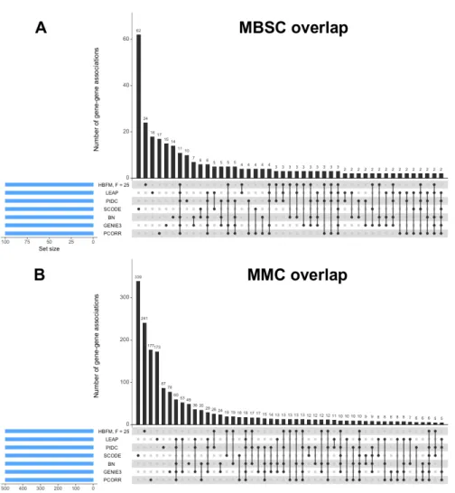
data . . . 52 3.2 UpSet plots of top gene-gene associations as determined by seven

dif-ferent methods for the MBSC and MMC datasets . . . 53 3.3 Comparison plots between the MMC dataset and one representative

PPD generated by HBFM . . . 54 3.4 Properties of PPD estimates from a sample of nine genes in the MMC

dataset . . . 55 4.1 Heatmaps of “true” correlation structures for treatment and control

groups in simulation studies . . . 71 4.2 Heatmaps of “true” differences between treatment correlation

struc-tures in Sim 3 and significant treatment differences identified by four differential network methods . . . 72 4.3 Heatmaps of “true” differences between treatment correlation

struc-tures in Sim 4 and significant treatment differences identified by four differential network methods . . . 73

(11)

CHAPTER 1

INTRODUCTION

For over a decade, RNA sequencing technologies have been instrumental in trans-forming our knowledge and understanding of transcriptomes. The analysis of data generated by these technologies has led to a plethora of novel biological findings ranging from the discovery of new transcripts to the identification of genes associated with specific diseases (Wang et al., 2009; Liu et al., 2015). Currently, RNA sequenc-ing experiments fall into one of two categories: bulk RNA sequencsequenc-ing (RNA-seq) or single-cell RNA sequencing (scRNA-seq). Traditional bulk RNA-seq experiments examine transcript abundance measurements that have been averaged over popula-tions of thousands, or even millions, of cells. In contrast, the more recent scRNA-seq experiments examine gene expressions from individual cells. While bulk RNA-seq studies have a longer history in the literature, scRNA-seq studies are rapidly gaining attention among researchers today.

What makes the future of scRNA-seq so promising is the unprecedented op-portunity to thoroughly investigate cellular functionality at the level of a single cell. Diverse gene expression patterns in cell populations that have previously seemed homogeneous are becoming exposed, allowing investigators to uncover solutions to unanswered questions across various fields of biology (Shapiro et al., 2013; Fan et al., 2015; Kanter and Kalisky, 2015). Nevertheless, the information collected from single-cell sequencing does present new computational and statistical challenges. Several intrinsic features of scRNA-seq data are not observed in bulk RNA-seq data (Figure

(12)

1.1), and so many of the well-established methods used in bulk RNA-seq studies are not suitable for seq studies. Thus, in order to take full advantage of scRNA-seq technologies, new statistical techniques need to be developed (Stegle et al., 2015; Bacher and Kendziorski, 2016).

Perhaps the most distinct characteristic of data generated by scRNA-seq is the abundance of zeros (Figure 1.1A). Specifically, the expression values of tran-scripts often exhibit bimodal distributions (Figure 1.1B) such that a gene can have high expression values for some cells but not be expressed in others (Shalek et al., 2013; Kharchenko et al., 2014). Although these expression patterns are due in part to technical variation and low concentrations of mRNA, they are also attributed to true biological differences between populations (or even subpopulations) of cells (Macaulay and Voet, 2014; Finak et al., 2015). Unimodal distributions typically used for the analysis of bulk RNA-seq data fail to capture the complex structure of scRNA-seq data, which bolsters the need for developing new methods specific to single-cell analyses.

Another prominent feature of scRNA-seq data is the increased cell-to-cell vari-ability (Figure 1.1C). Since information is being gathered from individual cells, dif-ferences in gene expressions across a single cellular population can now be observed. This means variation in scRNA-seq data can exist both between different groups of cells and within the same cellular population (Huang, 2009; Buettner et al., 2015; Ko-rthauer et al., 2016; Tirosh et al., 2016). Traditional bulk RNA-seq experiments often mask this heterogeneity by averaging out the gene expression measurements, and for that reason, bulk RNA-seq methods do not directly take the high cell-to-cell varia-tion associated with scRNA-seq into consideravaria-tion. Here, the need for new single-cell analysis methods is again highlighted by the inability of bulk RNA-seq methods to appropriately address the unique characteristics of scRNA-seq data.

(13)

that are differentially expressed between different populations of cells or construct-ing biological networks of genes within a population of cells, are also performed in scRNA-seq studies. Moreover, there are some tasks, such as identifying subpopula-tions of cells, that are unique to scRNA-seq experiments. Since bulk methods are not appropriate for analyzing single-cell data, new analytic tools specific to scRNA-seq are in high demand. The development of novel statistical techniques for the analysis of scRNA-seq data is gaining much attention, and research in this area is moving quickly. Some progress has already been made in this emerging area of research, but numerous opportunities still exist for the development of new single-cell methodology.

1.1

Differential Expression of Single-cell RNA Sequencing Data

A commonly performed task in sequencing analysis is the identification of genes that are differentially expressed (DE) across different populations of cells. Two of the most commonly referenced methods that have been designed specifically for differential expression analysis of scRNA-seq data are Single-Cell Differential Expression (SCDE; Kharchenko et al., 2014) and Model-based Analysis of Single-cell Transcriptomics (MAST; Finak et al., 2015). SCDE generates error models for each gene by using a mixture of a low-level Poisson distribution and a negative binomial distribution. The Poisson distribution is used to capture genes that are undetected across some of the cells, and the negative binomial distribution is used to address overdispersed expression counts commonly observed in sequencing data. MAST uses a two-part generalized linear model (hurdle model) to analyze continuous scRNA-seq expression levels, as opposed to analyzing discrete count values like SCDE. A logistic regression is initially used to model the proportion of cells that express a given gene, thereby addressing the overinflation of zeros observed in scRNA-seq data. Then, if a gene is expressed within a cell, a Gaussian distribution models the transformed expression level.

(14)

More recently, several other methods for detecting DE genes in scRNA-seq have also been proposed. The Beta-Poisson Single-Cell (BPSC) method in Vu et al. (2016) uses a generalized linear model framework with a beta-Poisson mixture model to compare mean expression values across cellular groups. Delmans and Hemberg (2016) introduced the Discrete, Distributional method for Differential gene Expres-sion (D3E), which also uses a beta-Poisson mixture model but compares gene expres-sion distributions using either the Kolmogorov-Smirnov test, the Cram´er-von Mises test, or the likelihood ratio test. A zero-inflated negative binomial model is utilized in DEsingle (Miao et al., 2018) to detect DE genes with likelihood ratio tests and estimate proportions of true zeros and dropout zeros.

Surprisingly, despite the variety of methods designed for differential expression analysis of scRNA-seq data, several studies have concluded that these methods do not perform much better than the bulk RNA-seq methods (Jaakkola et al., 2017; Miao and Zhang, 2016; Soneson and Robinson, 2018). Therefore, opportunities still exist for developing new methodology that will significantly outperform the bulk methods. In Chapter 2, a novel statistical model for high dimensional and zero-inflated scRNA-seq count data is introduced to identify differentially expressed genes across cell types. We adopt a hurdle model to address the overabundance of zeros in scRNA-seq data, and employ a correlated random effects structure guided by an initial supervised subpopulation clustering assignment to capture the observed cellular variability within treatment groups of cells.

1.2

Network Inference from Single-cell Gene Expression Data

Another common task in sequencing analysis is the construction of networks of genes with similar biological processes. These networks, which are often classified as ei-ther gene co-expression networks (GCNs) or gene regulatory networks (GRNs), pro-vide valuable insight into the functionality and mechanics of biological processes. In

(15)

GCNs, the edges that connect nodes (genes) within the network are considered to be “undirected” since they only indicate the relationships or dependencies between the co-expression of genes, not the underlying cause of these associations. This makes GCNs slightly different from GRNs, which connect nodes with directed edges that can be used to infer casual relationships (De Smet and Marchal, 2010). Network analysis is an important tool in the biomedical sciences because genes involved in the same biological pathway or have similar functionality tend to also have similar expression patterns (Eisen et al., 1998; Allocco et al., 2004). By examining GCNs and GRNs, researchers can gain a better understanding of the relationships and interactions be-tween sets of genes during different cellular functions and processes (Wolfe et al., 2005; Hecker et al., 2009; Wang et al., 2016).

Interestingly, research in designing new methodology for scRNA-seq gene net-working analysis has only recently been gaining attention in the literature. Lag-based Expression Association for Pseudotime-series (LEAP; Specht and Li, 2016) is a GCN method that determines gene co-expression by taking into account the possible lags in time that can be caused by cells being in different time points of their cell cycles. Introduced by Aibar et al. (2017), Single-Cell rEgulatory Network Inference and Clus-tering (SCENIC) constructs GRNs by first detecting potential sets of co-expressed genes within a population of cells and then performing a transcript factor enrichment analysis to identify and score significantly enriched gene sets. The Single-Cell Or-dinary Differentiation Equation (SCODE) algorithm from Matsumoto et al. (2017) uses linear ordinary differentiation equations to obtain an optimized square matrix that represents the regulatory relationships between transcription factors. Partial Information Decomposition and Context (PIDC; Chan et al., 2017) is an information theory based algorithm that utilizes partial information decomposition to identify GRNs.

(16)

scRNA-seq do not outperform methods developed for bulk RNA-scRNA-seq data (Chen and Mar, 2018). Thus, new network methods applicable to scRNA-seq data need to be devel-oped. In Chapter 3, a sparse Bayesian latent factor model is presented to explore the network structure associated with genes in a single population of cells. For a given cell, a set of shared latent factors adjusts the expression value for each gene, thereby accounting for the zero-inflation and overdispersion commonly observed in scRNA-seq data. A network structure is then inferred from the common factors between pairs of genes that impact their expressions.

1.3

Single-cell Differential Network Analysis

Methods for constructing GCNs and GRNs typically assume that the network struc-ture is being explored within one population of cells such as a single tissue type, environmental condition, or disease status. For some biological studies, however, it may be of greater interest to compare structures from different cellular populations. Different types of cells, or the same type of cell in different stages or conditions, may carry out different functions, and by performing differential network analysis between two (or more) gene-gene association or interaction networks, researchers can identify the parts of the network that are affected by these biological differences.

Most methods for examining differences between gene network structures have been developed in the context of microarray and bulk RNA-seq data. To our knowl-edge, the literature related to methodology developed for scRNA-seq differential net-work analysis is quite sparse. In fact, Chowdhury et al. (2019) provide an extensive review on differential co-expression analysis of gene expression data that highlights the need for more research in scRNA-seq methodolgy. The statistical framework de-veloped by Gill et al. (2010) for microarray gene expression data was utilized in Wang et al. (2017) to present proof-of-concept analyses for comparing network structures constructed from scRNA-seq data. Chiu et al. (2018) introduced the scRNA-seq-based

(17)

differential network (scdNet) analysis method to determine a sample size corrected gene-gene correlation matrix for each cellular state and identify gene-gene pairs that have significant changes between these states. The authors claim that scdNet is the first tool for differential network analysis of scRNA-seq data.

In Chapter 4, we expand upon the network model proposed in Chapter 3 to ex-amine differences in the underlying networks across two separate cellular populations. Under this model, the parameters that influence the latent factors are treatment-dependent to allow gene-gene co-expression calculations within each group of cells. The gene network structures can then be compared by analyzing credible intervals of the differences between the co-expressions of each group.

(18)

1.4

Figures

Figure 1.1: Comparisons between bulk RNA-seq and scRNA-seq data. (A) Proportion of zeros boxplots from a bulk (bulk1) and a single-cell (sc1) dataset. For each type of RNA-seq data, genes were sorted by their median expression values and groups were formed based on percentiles. (B) Estimated number of modes for the expression distributions of 1,000 randomly selected genes from three bulk and three scRNA-seq datasets. (C) Log variance density plots for all of the genes in the datasets from B. Densities were also created for the log variance of the scRNA-seq datasets when zeros were removed to illustrate the variation across the non-zero expression values.

(19)

CHAPTER 2

DETECTION OF DIFFERENTIALLY EXPRESSED GENES IN

DISCRETE SINGLE-CELL RNA SEQUENCING DATA USING A

HURDLE MODEL WITH CORRELATED RANDOM EFFECTS

1

2.1

Introduction

Rapidly emerging advances in next-generation technology have pushed single-cell analysis to the forefront of gene expression profiling experiments. Traditionally, tran-scriptomic studies have examined transcript abundance measurements averaged over bulk populations of thousands of cells. While bulk RNA sequencing (RNA-seq) mea-surements have been valuable in countless studies, they often conceal cell-specific het-erogeneity in expression signals that may be paramount to new biological findings. Fortunately, with single-cell RNA sequencing (scRNA-seq), transcriptome data from individual cells are now accessible, providing opportunities to investigate functional states of cells, identify rare cell populations, and uncover diverse gene expression pat-terns in seemingly homogeneous cell populations (Huang, 2009; Shapiro et al., 2013; Buettner et al., 2015).

One of the most commonly performed tasks in transcriptome expression pro-filing is the identification of genes that are differentially expressed (DE) across dif-ferent biological conditions, treatment groups, or cell types. For consistency in this

1_{Reproduced with permission from “Detection of differentially expressed genes in discrete}

single-cell RNA sequencing data using a hurdle model with correlated random effects” by Michael Sekula, Jeremy Gaskins, and Susmita Datta, 2019. Biometrics. DOI:10.1111/biom.13074.

(20)

manuscript, we will refer to the populations of cells being compared in a differen-tial expression analysis as treatment groups. Several popular methods for differendifferen-tial expression analysis of traditional bulk RNA-seq datasets currently exist, but these methods fail to capture the intrinsic characteristics that differentiate scRNA-seq data. The most prominent attribute of scRNA-seq is that a transcript can be moder-ately or highly expressed in some of the individual cells but not detected in others, re-sulting in a bimodal distribution of expression values (Shalek et al., 2013; Kharchenko et al., 2014). This expression pattern is caused by the low starting amounts of mRNA within each individual cell in combination with variation from biological and technical sources (Macaulay and Voet, 2014; Finak et al., 2015). The unimodal distributions used for the traditional differential expression analysis of RNA-seq data do not prop-erly model this inherent bimodal structure of scRNA-seq data. In addition, cell-to-cell variability in scRNA-seq has been shown to exist not only between different cellular populations but also within the same population of cells (Huang, 2009; Buettner et al., 2015). This observed heterogeneity is not directly addressed in traditional RNA-seq differential expression methods.

Because scRNA-seq datasets exhibit properties different from bulk RNA-seq datasets, new techniques for identifying DE genes specific to scRNA-seq data need to be developed (Stegle et al., 2015; Bacher and Kendziorski, 2016). Two commonly used methods that have been proposed to identify DE genes while taking into consideration the intricate nature of scRNA-seq data are SCDE (Kharchenko et al., 2014) and MAST (Finak et al., 2015). With the SCDE method, error models for each gene are first modeled using a mixture of a negative binomial distribution (to account for overdispersed expression counts from detected transcripts) and a low-level Poisson distribution (to accommodate genes that are undetected across some of the cells). Posterior probabilities of a given fold expression difference are then calculated to test genes for differential expression between two subgroups of cells. MAST is a

(21)

two-part generalized linear model (hurdle model) that analyzes continuous scRNA-seq expression levels, rather than discrete count values. A logistic regression first models the gene expression rate, and, conditioning on a cell expressing the given gene, a Gaussian distribution models the transformed expression level. Differential expression can then be tested using a likelihood ratio test.

In our view, a hurdle model structure (like MAST) is the best way to model such data with an overabundance of zeros. The components of a hurdle model are regression models (one for zero counts and one for expression values), which makes parameter estimation fairly straightforward and computationally simple compared to other types of methods. With a two component model, one can distinguish whether differences between treatment groups come from differences in the proportion of zeros, differences in actual expression, or both. Moreover, hurdle models are flexible and can adjust for potential experimental bias, such as dropout or cell size, with the addition of biological and/or technical covariates.

Rather than transforming the scRNA expression counts to continuous variables (as required in MAST), we adopt the hurdle model approach to directly model the discrete data. Consequently, we propose a mixed effect hurdle model for discrete scRNA-seq gene expression counts to detect genes that are DE between different treatment groups. The expression rate for a particular gene is first modeled with logistic regression to account for the high proportion of zeros in scRNA-seq data, and the expression count is then modeled with a zero-truncated negative binomial regression, conditional on the gene actually being expressed. Besides using discrete count data, another key difference between MAST and our proposed methodology is the incorporation of cell heterogeneity in a supervised manner. We utilize a random effects structure, guided by subpopulations of cells, to provide dependence across genes within a cell and across cells of a subpopulation. Finally, the third major difference between our method and MAST is that we implement a Bayesian approach

(22)

to estimate model parameters.

This manuscript is organized as follows. We define the hurdle model and introduce the structure of the correlated random effects (CRE) in Section 2.2. In Section 2.3, we present the methods for estimating model parameters and determining DE genes. Our proposed methodology is applied to both simulated and real data in Section 2.4, where we also compare the performance of our methodology to the performance of other commonly used methods for detecting DE genes. Finally, we conclude with a brief discussion of our results in Section 2.5.

2.2

Methodology

2.2.1 Model Structure

LetYgi be the expression count of geneg (g = 1, ..., G) in celli (i= 1, ..., N), andZgi indicate whether the gene is expressed within the cell. With this definition, Zgi = 1 when Ygi > 0, and Zgi = 0 when Ygi = 0. Defining θgi = P(Zgi = 1), the indicator variable Zgi follows Bernoulli(θgi), and the logistic model is defined as

logit(θgi) =β0Lg+XiβLg +ωiζgL, (2.1)

where Xi is a row from the design matrix consisting of a treatment group indicator and any other covariates of interest, such as cell size or estimated dropout rate. In Equation (2.1), we present the general case where Xi has more than one element, hence βL

g is a vector of regression coefficients. Also, we use the superscriptL on the

coefficients from the logistic model to distinguish them from the coefficients in the zero-truncated negative binomial regression.

The random effectωi for celli is included in the model to account for additional variability between cells and to induce correlation across genes. Depending on the

(23)

thus, we introduce a coefficient for the random effectsζL

g to represent a gene specific scaling factor for the random effects within the logistic regression component.

For the conditional expression counts, we define the negative binomial distri-bution as P(Ygi =y) = Γ(y+φg) y!Γ(φg) µgi µgi+φg y φg µgi+φg φg , y= 0,1, . . . , (2.2)

where µgi, φg > 0. Under this set-up, E(Y) = µgi and V ar(Y) = µgi + µ2

gi

φg,

mak-ing φg the overdispersion parameter. A modification to Equation (2.2) is needed to account for conditioning on a non-zero expression count (Ygi > 0); therefore, the zero-truncated negative binomial distribution is defined as

P(Ygi =y|Zgi= 1) = Γ(y+φg) y!Γ(φg) µgi µgi+φg y φg µgi+φg φg 1− φg µgi+φg φg , y= 1,2, . . . , . (2.3)

Using the distribution in (2.3), we have the following regression model for conditional expression counts:

log(µgi) = β0Cg+XiβgC +ωiζgC . (2.4)

Here, the superscript C indicates the coefficients in the count model (zero-truncated negative binomial regression). With this hurdle component, the regression coefficients in (2.4) can be interpreted as approximately representing a multiplicative effect on the expression count. Thus, if Xi1 is a dummy variable for the treatment indicator, β1Cg (the first element of vector β_gC) would approximately represent the log-fold change. The same random effect (ωi) used in the logistic model is also used here to control dependence across genes and dependence with the logistic model. The coefficient of the random effects ζC _{is representative of a scaling factor for} _ω _{per gene within the}

(24)

truncated negative binomial regression component.

2.2.2 Correlated Random Effects

It has been observed that within defined treatment groups of scRNA-seq experiments there exist subpopulations of cells with different expression patterns across different genes (Huang, 2009; Buettner et al., 2015). In order to account for this observation, we assume that the random effects of cells within a subpopulation are positively correlated, but between subpopulations, the random effects are independent. We refer to this model as CRE.

Before utilizing our CRE model, cells within each treatment group need to be clustered separately to formK0 subpopulations in the control group andK1 subpop-ulations in the treatment group. These subpopulation clusters can be identified with a suitable scRNA-seq clustering algorithm and then applied to our model structure. We must emphasize that our focus is not on how to perform a cluster analysis, but rather on how the results from a cluster analysis are incorporated into our model. Therefore, we assume that best practices (e.g., normalization, batch effect adjust-ments, etc.) have been followed before clustering to avoid additional influence of any biological and/or technical bias on the differential expression results.

Lettingkt(i) indicate the cluster assignment for celli in treatment t, we have

k0(i) andk1(i) representing the clusters/subpopulations within the control group and treatment group, respectively. Using this notation, each cellular random effect ωi is defined as the sum of two separate components: ωi =γt,kt(i)+ω

∗

i. Here,γt,krepresents the average random effect for the subpopulation k within treatment t, and ω_i∗ is the individual cellular adjustment for cell i within the subpopulation. With each γt,k following an independent and identically distributed (i.i.d.) Normal(0, σ2

t) and each

ω_i∗ following an i.i.d. Normal(0, σ_∗2), the correlation,ρt, between cells within the same subpopulation is thenρt =

σ2 t

σ2 t+σ∗2.

(25)

We note that the random effect ωi enters into the model through the terms

ωiζgL and ωiζgC. As ωi, ζgL, and ζgC are all estimated parameters, the individual ωi’s are, therefore, scale-unidentified. However, the relative contribution of γt,kt(i) to ωi is

identifiable, as will be the correlation ρt. To facilitate interpretation, the estimated

ωi’s can be post hoc rescaled to have variance one.

For special cases, such as datasets with large numbers of cells, or situations when an initial clustering is not preferred, the correlations between random effects can be removed and one can simply assume that all of the random effects are independent of each other. Under this assumption, eachωi simply follows an i.i.d. Normal(0, σ2). We refer to this model choice as independent random effects (IRE).

2.3

Model Inference

2.3.1 Parameter Estimation

A Bayesian approach is utilized to estimate the parameters of our proposed model. While a seemingly straight-forward technique for obtaining these parameter estimates is Markov chain Monte Carlo (MCMC) sampling, it may take days of computational time for this iterative process to generate enough samples to reasonably estimate our model parameters on large scRNA-seq datasets. This makes an MCMC approach impractical compared to the computational time of methods currently available for identifying DE genes. If time is not a factor, researchers may still choose to utilize full MCMC to obtain parameter estimates and model inference.

Instead of time-consuming MCMC, we use variational inference (VI) to ap-proximate the posterior distribution and obtain parameter estimates more quickly. VI has been recently proposed as a computationally faster alternative to MCMC for solving Bayesian problems involving large data (Blei et al., 2017). Briefly, mean-field variational Bayes approximates the usual posterior distribution p(Θ|y) with a

(26)

distri-bution q(Θ) that assumes all components of Θ are independent, q(Θ) = Q

jqj(Θj). This leads to an optimization problem of finding theq(Θ) =Q

jqj(Θj) that is closest in Kullback-Leibler divergence to the true posterior.

Introduced by Kucukelbir et al. (2015), automatic differentiation variational inference (ADVI) is a user-friendly method that automatically generates an algorithm to solve this optimization problem. In essence, each qj(·) is assumed to be a normal distribution on a suitable transformation of Θj. Optimizing the parameters of these normal distributions is accomplished using a stochastic gradient ascent algorithm to maximize the evidence lower bound (ELBO). Monte Carlo integration approximates the expectations of the ELBO and automatic differentiation computes the gradi-ents that are maximized. We implement the mean-field algorithm of ADVI in R (R Core Team, 2018) through the package rstan (Stan Development Team, 2018). After achieving convergence to the approximate posterior with rstan’s ADVI algorithm, parameter samples are drawn independently from q(Θ) and provided to the user as approximate posterior samples from p(Θ|y).

To complete the specification of our Bayesian model, we need prior distribu-tions for the remaining parameters. The regression coefficients in both the logistic regression and the zero-truncated negative binomial regression are given weakly infor-mative Cauchy priors (Gelman et al., 2008). The intercept terms have Cauchy(0,10) priors, while the remaining coefficients have Cauchy(0,2.5) priors. The lognormal distribution is used as the prior for the overdispersion parameter φg, with the hyper-parameters λ1and λ2 defined as

φg ∼Lognormal(λ1, λ2),

λ1 ∼Cauchy(0,10),

(27)

Sensitivity analysis with the case study data (see Appendix D) indicates replacing the

λ2 prior with Inverse Gamma(1,1) has little effect on the final differential expression results. In addition, the variance parameters for the cellular random effects,σ2

t andσ∗2,

have Inverse Gamma(1,1) priors. By choosing this prior for the variance parameters, the prior for ρt, the correlation between cells within the same cluster, is Beta(1,1).

2.3.2 Testing for Differential Expression

Typically, the target of inference in scRNA-seq studies is to determine if genes from two treatments are “differentially expressed” (DE), that is, they follow different dis-tributions. In our modeling framework, the difference in the distributions between treatments is controlled by the pair of regression coefficientsβL

1g and β1Cg of the treat-ment group indicator. A gene is considered to be DE if at least one of these parame-ters is non-zero. That is, we need to test H0 :β1Lg =β1Cg = 0 against the alternative. While we develop our model and estimate parameters under the Bayesian paradigm, we choose to perform hypothesis testing under the standard frequentist framework as most researchers are more familiar with this approach.

We defineBc_gto be the two-dimensional vector consisting of the point estimates

of βc₁L_g and βc₁C_g (the treatment effect coefficients from the logistic and count models

for geneg), and letVg represent the estimate of the covariance matrix, as determined

empirically from the posterior samples (provided as output by Stan) of these two coefficients. Wang and Blei (2019) have established that the variational posterior

q(Θ) is asymptotically normal with a random mean centered at the true parameter value. Thus, under the null hypothesis that βL

1g = β1Cg = 0, the test statistic Wg =

c

Bg

T V−1

g Bc_g will asymptotically follow a chi-square distribution with two degrees of

freedom. IfWg is larger than the appropriate critical value, we rejectH0 and conclude that gene g is differentially expressed; a p-value can also be obtained.

(28)

2.4

Applications

2.4.1 Simulation Studies

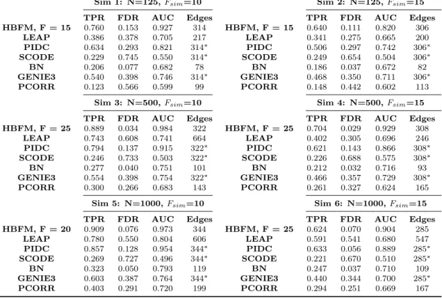
To evaluate performance, we applied our method to simulated data generated from our proposed model. We considered scenarios when the true subpopulations had equal sizes (same number of cells per subpopulation) and unequal sizes (different number of cells per subpopulation). An additional simulation was run using data generated with the Splat simulation design (Zappia et al., 2017) to evaluate the performance of our models on data simulated from a structure that differs from our proposed methodology. Small datasets (100 cells and 10,000 genes) were analyzed to illustrate the feasibility of our methods, while larger datasets (1,000 cells and 10,000 genes) were analyzed to demonstrate their practical utility. Details on these simulation designs are available in the Appendix.

Two versions of the proposed hurdle model, the CRE model and the IRE model, were evaluated under these different simulation scenarios. In our model ma-trix, we included the treatment group indicator and the cellular detection rate (CDR) as covariates. The CDR for cell i is the sample proportion of genes that have a non-zero count, CDRi = 1 G G X g=1 Zgi, (2.5)

and has been presented by Finak et al. (2015) as an important source of variability that captures variation due to biological and technical factors, such as cell volume and dropout. Since our model does not inherently distinguish between true biological zeros and technical zeros, including CDR as a covariate will help control for expression differences due to these unwanted sources of variation. To demonstrate that the addition of random effects actually improves upon a model that includes CDR, we also tested our proposed methodology using only fixed effects (i.e., removing theωiζg

(29)

terms from (2.1) and (2.4)). We refer to this model as no random effects (NRE). When applying the CRE model, clusters within each treatment group were as-signed by the SNN-Cliq algorithm (Xu and Su, 2015) and the SC3 algorithm (Kiselev et al., 2017). SNN-Cliq requires the number of nearest neighbors to find a clustering structure, and so the number of nearest neighbors was set to the default value of three. We also set the number of nearest neighbors to seven in the hurdle model simulations to obtain fewer numbers of clusters within each treatment group. Since the Splat simulation does not inherently create subpopulations, we only considered three near-est neighbors. The SC3 algorithm, on the other hand, requires the number of clusters to be specified. Therefore, we utilized SC3’s option to estimate the optimal number of clusters for each treatment group in each simulated dataset. As an alternative clustering option in the hurdle model simulations, we also estimated the model under the true data-generating subpopulation assignments to gauge performance when the actual clustering structure is known.

In addition to evaluating the performance of our methodology, we also compare our proposed models to methods commonly used in the literature. The methods for scRNA-seq differential expression of MAST and SCDE were examined in these studies along with two methods designed for bulk RNA-seq differential expression: edgeR (Robinson and Smyth, 2007) and DESeq2 (Love et al., 2014). The covariate of CDR was also implimented in the model matrix for MAST as described in the MAST package vignette for the MAIT data analysis (McDavid et al., 2019).

Instead of utilizing raw discrete counts, the two clustering algorithms and MAST require continuous expression data. To that end, a trimmed mean of M-values normalization was first applied to the simulated datasets to account for between-sample bias, and the adjusted count values were then scaled to counts per million with the edgeR package (2019), thereby accounting for differences in library size.

(30)

DE genes were determined at a false discovery rate (FDR) of 0.05 for each method. We used the measures of true positive rate (TPR), false positive rate (FPR), observed FDR, area under the receiver operating characteristic curve (AUC), and the number of identified DE genes to compare methods. Summaries of these measures for all simulations are provided in Table 2.1.

In all hurdle model simulations, the NRE model was unable to control FDR at a nominal rate and had approximately twice the FDR as both CRE and IRE. This result was observed even when the “true” subpopulation structures were sim-ulated with different numbers of clusters and with higher within-cluster correlations (Appendix A). Therefore, the addition of random effects to our methodology helps control the FDR when underlying subpopulations exist. When comparing the random effects models, CRE and IRE have similar performances in the smaller hurdle model simulations, with CRE having slightly lower FDRs. However, this difference becomes more evident in the larger datasets. Hence, the correlated random effects do a better job at controlling the FDR to a nominal level than the independent random effects. Moreover, the correlation structure of CRE is quite robust as the performance of this method is generally unaffected by the initial clustering of cells within each treatment group.

Even though the Splat design does not simulate a subpopulation structure, CRE and IRE still obtain higher TPRs and larger numbers of detected DE genes compared to NRE. Additionally, the Splat simulations demonstrate that bias is not introduced if a clustering structure is input into CRE when the dataset does not inherently have “true” subpopulations. In fact, the results from IRE and CRE are nearly identical in the larger Splat simulation.

When comparing our methodology to the other methods for detecting DE genes, CRE and IRE consistently identified large numbers of DE genes with high power (TPR), and detected more DE genes than MAST across all simulations. The

(31)

FDR of our models is well maintained at the nominal level (as is MAST), but SCDE and the bulk methods consistently fail to control FDR. Regarding the AUC, our method outperforms the competing approaches (both bulk and scRNA) across all scenarios. Because it also relies on a hurdle model specification, we do note that MAST is somewhat competitive in AUC when the data-generating mechanism is our hurdle model. Nevertheless, MAST performed poorly in the Splat simulations as it had the lowest AUC out of all the considered methods. These overall trends were also observed when different subpopulation structures were simulated (Appendix A).

2.4.2 Case Studies

To further illustrate our proposed methods, we analyzed the mouse embryonic cell (MEC) dataset (Islam et al., 2011), which contains expression counts of 92 single-cells generated from two different cell types: 48 stem cells and 44 fibroblast cells. This dataset was obtained from the Gene Expression Omnibus (GEO) database under accession number GSE29087. Genes not expressed in at least 20% of the cells were removed, leaving 7,912 genes in the analysis. SNN-Cliq with five nearest neighbors was used to generate cluster assignments within each treatment group to form three clusters within the stem cells and two clusters within the fibroblast cells for input into our CRE model. It has been noted that if the number of nearest neighbors is too large, clusters formed by SNN-Cliq may not be thoroughly separated, and if the number of nearest neighbors is too small, a true cluster may be split into multiple parts (Xu and Su, 2015). Based on visual inspections of different SNN-Cliq clustering assignments, we determined that five nearest neighbors was a reasonable choice (not too small, not too large) for clustering this particular dataset.

We also analyzed a Drop-seq dataset containing single-cell expressions of 2,000 human mammary epithelial cells (HMEC) expressing either exogenous wild type or mutant histone H2B to demonstrate the utility and scalability of our methods on big

(32)

data. Details of the Drop-seq procedure are provided in Appendix C. This dataset is quite sparse, so we chose to filter out genes not expressed in at least 50 cells (2.5% of the total cells), leaving a total of 3,139 genes in the analysis. Four cells from the dataset were also removed because they had a library size of zero after gene filtering. To define the random effect structure of CRE, we utilized SC3 to cluster the 999 wild type cells into seven subpopulations and the 997 mutant cells into nine subpopulations. These clustering results were taken from a previous cluster analysis performed on this data by our research group (see Appendix C).

The differential expression methods used in the simulation studies, excluding NRE, were run in R independently using a single core of a system with an Intel Core i7 processor (3.5 GHz) and 8 GB of RAM. Based on the results in Table 2.2, the computational time required for our methods is very reasonable for a Bayesian analysis on datasets of these sizes. MCMC sampling would take days of running time before obtaining enough samples for an appropriate analysis. While both CRE and IRE take longer than the other methods on the smaller MEC dataset, they do scale better, and are also faster, than SCDE and DESeq2 on the larger HMEC data.

In terms of the number of DE genes detected, CRE and IRE performed simi-larly in the case studies, which is consistent with the simulation results. CRE iden-tified 4,927 and 1,698 DE genes in the MEC and HMEC datasets, respectively, while IRE identified 4,947 and 1,696 genes. The overlap of genes was also very high in the case studies for these methods (4,808 in the MEC data, and 1,640 in the HMEC data). Nevertheless, the simulation studies do show that CRE outperforms IRE in terms of FDR, especially in larger datasets. For that reason, we focus the rest of our discussion in this section on interpreting the CRE results.

Figure 2.1 displays the UpSet plots (Lex et al., 2014) for the intersection of DE genes identified by the different methods in the MEC and HMEC analyses. Just like the simulation studies, our method detects a larger number of DE genes than

(33)

most methods in these case studies. In the MEC data, CRE detected the most DE genes, and surprisingly, the other two scRNA-seq methods detected fewest DE genes. CRE was second, only to edgeR, in the number of identified DE genes in the HMEC dataset, while DESeq2 detected very few DE genes compared to the other methods.

As CRE identified a large number of unique DE genes in the MEC analysis relative to the competing models, we further examined the 1,335 genes uniquely identified as DE by CRE to determine if they have any biological relevancy. For comparison purposes, we also examined the 293 genes identified only by edgeR and the 172 genes detected only by DESeq2 (Appendix D). We found that the subset of genes detected by CRE are associated with more clusters of enriched gene ontology (GO) categories than the subsets of genes detected by the other two methods. Thus, not only is CRE able to identify a larger number of DE genes, but these genes also have roles in similar biological functions and processes.

From a statistical standpoint, our methodology determines DE genes by taking into account the difference in the proportion of zeros between the two treatments as well as the difference in the average counts conditional on the gene being expressed. This is why the CRE model detects different genes than the other methods, particu-larly in the MEC analysis. In Figure 2.2, we present the log2 fold change (log2FC) against the log2 ratio of the proportion of zeros (log2PZ) for the top 500 genes de-termined by each method in the MEC data.

Figure 2.2 highlights the ability of our methodology to incorporate both com-ponents of the hurdle model (zero counts and expression values) when identifying DE genes. Out of the top 500 genes identified by CRE, 433 of them had notable differences in the number of zeros across groups as indicated by the absolute value of the log2PZ being greater than one (i.e., one treatment group has more than twice the number of zeros than the other). In addition, all but one of those genes also had an absolute value of log2FC greater than one. Therefore, most of the top DE genes

(34)

identified by CRE were not only different in terms of the number of zeros between the stem and fibroblast cells, but also in terms of the expression values between the treatment groups.

The other methods did not detect as many DE genes with notable differences in the proportion of zeros between treatments. Out of all of the methods, MAST detected the fewest number of genes with an absolute value of log2PZ greater than one. This showcases the superiority of our model in the MEC analysis since MAST also takes into account the differences in the proportion of zeros when determining DE genes. Only 238 out of the top 500 genes identified by MAST had more than a twofold difference in the proportion of zeros between treatments, whereas DESeq2, edgeR, and SCDE identified 342, 331, and 290 genes that satisfied this criterion, respectively.

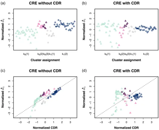
Lastly, to demonstrate the role of the random effects in our methodology, we ran an additional analysis of the MEC data with a model matrix that only included the treatment group indicator covariate. This produced an estimate ofωi that is free from potential feedback from the CDR covariate. We see from Figure 2.3A that the estimates of the random effects within the same treatment subpopulation tend to have similar values when CDR was not included in the model matrix. The estimated within subpopulation variance was 0.40 while the between subpopulation variance was 14.13. A majority of the random effect estimates for Subpopulation 1 in the stem cells and Subpopulation 1 in the fibroblast cells were negative, whereas the estimates of the random effects for the other subpopulations were mostly positive. When CDR was included in the model (Figure 2.3B), there appeared to be less separation between cluster/subpopulation means, as this information is now accounted for through CDR. For these estimates, the within subpopulation variance was 0.91 and the between subpopulation variance was 2.84.

(35)

the normalized CDR to display the relationship between these two terms. With CDR not included in the model matrix, the random effect estimates tended to be fairly similar to their corresponding CDR counterparts. The linear association between these terms suggests that they are able to capture similar cellular variability. When CDR was included in the model, there is no longer a discernible trend between the random effects and CDR, indicating that the random effects terms are accounting for some secondary source of cellular variation beyond the fraction of genes expressed.

2.5

Discussion

In this manuscript, we have introduced a mixed effects hurdle model for detecting genes that are DE between treatment groups of cells in discrete scRNA-seq data. The hurdle model structure handles the abundance of zero counts typical of scRNA-seq, while the CRE help account for the cell-to-cell heterogeneity that has been frequently observed within treatment groups of cells. One may also choose to use our proposed hurdle model with independent random effects for situations where clustering may not be suitable. Both of our proposed models (CRE and IRE) outperformed two methods developed for detecting DE genes in scRNA-seq data (MAST and SCDE) and two methods designed for bulk RNA-seq data (edgeR and DESeq2) in the simulation studies. We recommend using CRE over IRE when possible as it tends to have lower FDRs.

Our proposed methodology is comparable in structure to that of MAST, de-veloped by Finak et al. (2015), which is also a hurdle model but for continuous data. We likewise incorporate the covariate of CDR (Equation (2.5)) into our model matrix to help control for the expression differences due to unwanted sources of variation. Nevertheless, our methodology is unique because it (1) analyzes discrete count data rather than continuous data that has already been transformed, (2) incorporates a novel correlated random effect structure to capture additional sources of variation, and

(36)

(3) utilizes a Bayesian approach to parameter estimation. These three key differences lead to the detection of more DE genes and higher TPRs and AUCs than MAST, as illustrated in the simulation studies. The MEC data analysis also demonstrates that our model can be more sensitive when detecting differences in the proportion of ze-ros. Therefore, despite the similarities in motivation, our methodology demonstrates superior performance over MAST.

We additionally note that we utilize a VI technique to quickly obtain samples of parameter estimates from an approximate posterior distribution rather than a typical MCMC sampling on the true posterior. However, there has been discussion in the literature regarding the accuracy of variance estimates under mean-field variational Bayes. Recently, Wang and Blei (2019) show that VI can recover the diagonal of the concentration (inverse covariance) matrix, but since the off-diagonal elements of concentration are set to zero, the marginal variances may be underestimated.

For this reason, some have argued that mean-field variation inference may not produce appropriate testing conclusions (e.g., Kucukelbir et al., 2017). Alterna-tive approaches include running full MCMC or estimating parameter variances by bootstrapping treatment assignments (Chen et al., 2018), although both would be enormously computationally expensive. However, based on our empirical work in Section 2.4, we emphasize that we are able to accurately estimate the regression pa-rameters in this context and that our hypothesis tests maintain the required FDR and achieve higher power than the competing scRNA methods. Thus, we conclude that our proposed methodology for detecting DE genes from single-cell RNA represents a new and powerful strategy for this biologically important problem.

2.5.1 Software Availability

The R package that implements our proposed methodology is maintained at github.com/mnsekula/scREhurdle.

(37)

2.6

Tables and Figures

Hurdle model: Equal clusters (N= 100) Hurdle model: Equal clusters (N= 1000)

TPR FPR FDR AUC DE Genes TPR FPR FDR AUC DE Genes

CRE, SC3 0.682 0.010 0.046 0.958 1548 0.751 0.016 0.056 0.965 1746 CRE, NN=3 0.682 0.009 0.045 0.959 1547 0.752 0.015 0.058 0.966 1739 CRE, NN=7 0.682 0.010 0.046 0.958 1550 0.751 0.015 0.058 0.965 1741 CRE, TRUE 0.682 0.010 0.047 0.958 1551 0.752 0.016 0.059 0.965 1749 IRE 0.686 0.011 0.050 0.958 1564 0.754 0.026 0.078 0.960 1830 NRE 0.669 0.019 0.086 0.947 1591 0.745 0.047 0.168 0.942 1965 MAST 0.594 0.007 0.038 0.948 1337 0.693 0.008 0.039 0.962 1563 SCDE 0.126 0.094 0.200 0.646 974 0.308 0.280 0.396 0.601 2756 DESeq2 0.402 0.058 0.321 0.777 1304 0.426 0.084 0.394 0.767 1549 edgeR 0.396 0.073 0.377 0.764 1400 0.488 0.148 0.504 0.740 2161

Hurdle model: Unequal clusters (N= 100) Hurdle model: Unequal clusters (N= 1000)

CRE, SC3 0.681 0.010 0.049 0.957 1550 0.572 0.017 0.074 0.924 1367 CRE, NN=3 0.680 0.010 0.049 0.957 1547 0.573 0.018 0.077 0.923 1372 CRE, NN=7 0.681 0.010 0.049 0.957 1550 0.573 0.018 0.079 0.923 1374 CRE, TRUE 0.681 0.010 0.049 0.957 1549 0.573 0.017 0.076 0.924 1365 IRE 0.684 0.011 0.051 0.957 1560 0.579 0.026 0.097 0.919 1444 NRE 0.669 0.023 0.097 0.945 1616 0.573 0.050 0.209 0.894 1610 MAST 0.587 0.007 0.038 0.947 1320 0.468 0.007 0.048 0.914 1066 SCDE 0.165 0.130 0.257 0.631 1353 0.364 0.343 0.554 0.545 3340 DESeq2 0.411 0.074 0.361 0.766 1442 0.378 0.151 0.549 0.684 1941 edgeR 0.407 0.087 0.406 0.754 1525 0.439 0.214 0.607 0.667 2543 Splat (N= 100) Splat (N= 1000)

CRE, SC3 0.475 0.006 0.051 0.924 576 0.434 0.004 0.041 0.840 539 CRE, NN=3 0.475 0.006 0.052 0.923 576 0.434 0.004 0.041 0.841 540 IRE 0.501 0.008 0.063 0.923 615 0.434 0.004 0.041 0.841 540 NRE 0.404 0.007 0.063 0.910 497 0.373 0.003 0.031 0.828 459 MAST 0.220 0.002 0.032 0.879 274 0.287 0.003 0.037 0.795 355 SCDE 0.254 0.002 0.028 0.917 303 0.287 0.001 0.010 0.826 294 DESeq2 0.601 0.042 0.215 0.887 892 0.450 0.019 0.149 0.814 634 edgeR 0.740 0.076 0.297 0.911 1219 0.563 0.062 0.317 0.818 987

Table 2.1: Results of performance measures from simulation studies. The subpopula-tion structure for the CRE model was input using either SC3, SNN-Cliq with 3 nearest neighbors (NN=3), 7 nearest neighbors (NN=7), or the true simulated subpopulation assignment (TRUE).

CRE IRE MAST SCDE DESeq2 edgeR

MEC data 38.4 40.1 1.2 23.6 0.8 0.1

HMEC data 77.6 69.7 2.3 107.9 392.8 0.9

(38)

Figure 2.1: UpSet plots of DE genes as determined by five different methods for both the MEC and HMEC datasets. Numbers in parentheses represent the total number of DE genes identified by the corresponding method. This figure appears in color in the electronic version of this article.

(39)

Figure 2.2: Scatterplots of the log2 proportion of zeros ratio (log2PZ) on the x-axis and the log2 fold change (log2FC) on the y-axis for the top 500 most DE genes in the MEC dataset as determined by the five different methods for detecting DE genes. Ratios compare stem cells to fibroblast cells and the labels in each section of the plot represent the number of genes in that section. This figure appears in color in the electronic version of this article.

(40)

Figure 2.3: Random effect estimates,ω_bi, for the cells in the MEC dataset with points colored according to cluster assignments determined by SNN-Cliq. (A, B) Plots of normalizedω_bi estimates by subpopulationkt(i) wheret= 0 for stem cells (represented by triangles) and t = 1 for fibroblast cells (represented by circles). (C, D) Plots of normalized ω_bi estimates vs. normalized CDR. This figure appears in color in the electronic version of this article, and color refers to that version.

(41)

CHAPTER 3

A SPARSE BAYESIAN FACTOR MODEL FOR THE

CONSTRUCTION OF GENE CO-EXPRESSION NETWORKS

FROM SINGLE-CELL RNA SEQUENCING COUNT DATA

3.1

Background

Deriving co-expression networks from gene expression data is a primary goal in nu-merous biological studies. These networks, which are commonly referred to as gene co-expression networks (GCNs), are constructed by identifying pairs of genes that have significant associations between their expression profiles across samples. Genes are represented by nodes in GCNs and co-expression values are represented by edges that connect pairs of nodes. These edges are undirected to indicate the relationships or dependencies between genes, not the underlying cause of these associations. This makes GCNs different from gene regulatory networks, which have directed edges to infer casual relationships (De Smet and Marchal, 2010). As demonstrated in Eisen et al. (1998), genes with similar expression patterns tend to be involved in similar cellular processes and functions. Therefore, researchers are able to identify novel in-teractions and relationships between genes by exploring GCNs (Wolfe et al., 2005; Wang et al., 2016).

Many of the statistical methods for building GCNs have been developed for analyzing data consisting of expression values averaged over bulk populations of cells, such as microarray or bulk RNA sequencing; however, advancements in technology

(42)

now allow researchers to obtain expressions at the level of a single cell. By gathering information from individual cells, new opportunities to study cellular heterogeneity are presented. This is of particular interest in GCNs since mapping gene expressions across different states of cells can lead to a better understanding of the biological mechanisms behind this heterogeneity (Fiers et al., 2018). Single-cell RNA sequencing (scRNA-seq) provides new and exciting opportunities to examine biological processes at a high resolution, yet at the same time, this data presents new statistical and com-putational challenges (e.g., zero-inflation, high cell-to-cell variability, multimodality) that have not been previously faced with bulk sample data (Bacher and Kendziorski, 2016). Therefore, network algorithms initially developed for bulk samples are often not suitable for single cell analysis (Blencowe et al., 2019).

Some algorithms for network analysis in scRNA-seq data have been recently proposed, but these methods fail to outperform general methods developed for bulk sample data Chen and Mar (2018). To that end, we present a sparse hierarchical Bayesian factor model to explore the network structure associated with genes. The latent factors in our model adjust the gene expressions for each cell to help accom-modate for the zero-inflated and overdispersed attributes of scRNA-seq data, and a GCN structure is constructed by examining the shared factors between pairs of genes. This manuscript is organized as follows. We define our proposed model and GCN inference in Section 3.2. In Section 3.3, we apply our method to both simulated and real data and also compare the performance of our methodology to the perfor-mance of other network methods. Finally, we conclude with a brief summary in the Section 3.4.

(43)

3.2

Methods

3.2.1 Hierarchical Bayesian Factor Model

Let Ygi be the (count) expression for gene g (g = 1, . . . , G) in cell i (i = 1, . . . , N). We assume each expression comes from the Poisson(µgi) distribution, where the mean

µgi is modeled through the representation

µgi=βg F Y f=1 expn− φf 2 |αgf| o λ αgf if . (3.1)

Here, the parameter βg denotes the average expression for gene g. For each cell i, there are F associated factors λi ={λi1, . . . , λiF}that impact the expression. These factors are strictly positive and come from a Lognormal(0, φf) distribution. We can think of each factor as representing a distinct attribute (e.g., cell stage, pseudotime point) that will only influence a specific set of related gene expressions. The exponent of thefth factorλif isαgf ∈ {−1,0,1}, and by using this set of discrete exponents for the factors, the expression for gene g is impacted only by the factors with αgf =−1 or 1. The adjustment term of exp{−φf

2 |αgf|}is included in Equation (3.1) to ensure that E(Ygi) is equal to βg (after marginalizing out λi) regardless of the αgf values.

Our defined factor structure provides the flexibility required to account for the typical cell-to-cell variability of scRNA-seq data. For a givenf,λif is unique to each cell and is only activated for a particular gene whenαgf 6= 0. If the activated factors

λ αgf

if for a given gene are much smaller than 1 (near zero), thenµgi will be very small and account for the high proportion of zeros typical of this data. Conversely, very large values of the factors will increaseµgi(relative to the baselineβg) and accommodate the occasional extremely large count. We note here thatYgifollows a Poisson distribution conditional on the λi terms. However, the variance of Ygi, marginal on λi, is equal

to βg +βg2 exp{−φf|αgf|} −1

(44)

overdispersed. So, despite the choice of Poisson for the distribution of the count, our model is able to capture the high proportion of zeros and large variance typical of scRNA data.

To finish specification of our Bayesian model, prior distributions for the remain-ing parameters must be defined. We use a conditionally conjugate, non-informative prior for the average expression of gene g,βg ∼Gamma(0.001,0.001). The hierarchi-cal prior structure for the shierarchi-cale parameter of the factors is φf ∼ Lognormal(h1, h2), where h1 ∼ N ormal(0,100) and h2 ∼ Inverse Gamma(1,1). For the exponent pa-rameters, the prior is |αgf| ∼ Bernoulli(θf) with θf ∼ Beta(1,1). Here, we define

P(αgf = 1) =P(αgf =−1) = θf

2. Consequently,P(αgf = 0) = 1−θf. The number of associated factorsF is often unknown, but one can fit multiple models with different numbers of factors and choose the most suitable model based on a comparison of a model selection statistic such as the Deviance Information Criterion (DIC) described in Gelman et al. (2004). Throughout the manuscript, we will refer to our hierarchical Bayesian factor model as HBFM.

3.2.2 Network Structure

Posterior samples for model parameters are obtained with the Markov chain Monte Carlo (MCMC) algorithm defined later in Section 3.2.3. At each iteration of the MCMC, a correlation matrix is computed based on the current set of parameters, and we infer a GCN by examining the posterior distribution of this correlation matrix. Under our proposed model, the sparseα={αgf}(g,f)matrix imposes a crude network structure on the gene expressions. Consider two genes g and g0, where g 6= g0. If

αgfαg0_f 6= 0 for somef, the expressions Y_gi and Y_g0_i are both impacted by the shared

factor λif. Conversely, if genes g and g0 have no shared factors (αgfαg0_f = 0 for all f), these genes are conditionally independent. To quantify the association between gene g and gene g0, we examine the correlation (after marginalizing outλi) between

(45)

the values of log(µgi) andlog(µg0_i).

We motivate our decision to use this specific correlation structure by consid-ering the matrix A˜ = ααT_{. The (}_{g, g}0_{) element of this} _G_×_G _{matrix provides of}

a summation of the associated factors that are active in both genes g and g0 since ˜

ag,g0 =PF

f=1αgfαg0_f. When ˜a_g,g0 >0, the two genes have more factors with the same

association (i.e., αgf = αg0_f = 1 or α_gf = α_g0_f = −1) than factors with opposite

associations (i.e., αgf = 1 and αg0_f = −1 or vice versa). Conversely, when ˜a_g,g0 <0,

the genes have more factors with opposite associations than factors with the same association. If ˜ag,g0 = 0, then either no factors are in common between the genes or

the number of factors with the same association is equal to the number of factors with opposite associations for those genes.

By recognizing that factors with a larger variance φf will have a greater influ-ence on the joint expression, we can weigh the shared factors by their variance. In fact, this weighted expression is exactly equal to the the covariance (marginally over λi) betweenlog(µgi) and log(µg0_i),

Covlog(µgi), log(µg0_i)=

F

X

f=1

φfαgfαg0_f .

The active factors also increase the variance forlog(µgi),

V arlog(µgi) = F X f=1 φfα2gf ,

which is important when addressing the zeros and overdispersion of scRNA-seq data. From these covariance and variance expressions, the correlation between log(µgi) and

(46)

Corrlog(µgi), log(µg0_i) =ρ_gg0 = PF f=1φfαgfαg0f r PF f=1φfα2gf PF f=1φfα2g0_f . (3.2)

We illustrate the mechanics of this correlation structure by considering just one factor f. If gene g and gene g0 have the same association with this given factor, the correlation betweenlog(µgi) andlog(µg0_i) is 1. When geneg has a positive association

with factor f and gene g0 has a negative association with factor f, the correlation is −1. Additionally, if factor f is inactive for either of the genes, the correlation is 0. The significance of each correlation is determined by analyzing the the credible interval (CI) of ρgg0 in the posterior distribution, as described in Section 3.2.4.

We note that each gene must have at least one active factor for our correlation structure in Equation (3.2) to be defined since V ar

log(µgi)

is equal to 0 if all of the factors are inactive. Utilizing the correlation structure (after marginalizing out λi) between Ygi and Yg0_i would avoid this issue, but the additional β_g term in the

variance leads to a correlation structure dependent on the average expression for each gene. For this reason, we do not focus on the correlation structure between Ygi and

Yg0_i. Throughout, if (3.2) is 0

0, we define this correlation as zero to match the zero value for Corr(Ygi, Yg0_i).

3.2.3 Model Inference

The posterior distribution for our hierarchical Bayesian model is complex, and so MCMC is required for inference. For simplicity in our posterior distribution notations, let ψgif =Q_f0₆₌_fexp

− φf0

2 |αgf0| λ αgf0

if0 . We utilize an MCMC sampler that iterates

through the following steps: 1. For g = 1, . . . , G, update

(47)

2. For f = 1, . . . , F, update θf ∼Beta 1 +PG_g₌₁|αgf| , 1 +G−PG_g₌₁|αgf|

. 3. For all g, f, sample αgf from a multinomial distribution with

p(αgf = 0| · · ·) = _A₊_BA₊_C,

p(αgf = 1| · · ·) = _A₊B_B₊_C,

p(αgf =−1| · · ·) = _A₊_BC₊_C. Here, A, B, and C are defined as

A= (1−θf)exp −βg PN i=1ψgif , B = θf 2 exp−βgPN_i₌₁exp − φf 2 λifψgif , C = θf 2 exp−βgPN_i₌₁ exp{−φf₂ } λif ψgif . 4. Update h1 ∼N ormal(₁_/₁₀₀₊1/h2_{F /h} 2 ∗ PF f=1log(φf),(1/100 +F/h2) −1_).

5. Update h2 ∼Inverse Gamma(F₂ + 1, PF

f=1(log(φf)−h1)2 2 + 1).

6. For f = 1, . . . , F, use a Metropolis-Hastings step to update φf. The posterior distribution forφf is p(φf| · · ·)∝φ −N 2−1 f exp n −φf 2 PG g=1 PN i=1|αgf|yg