Application Of Differential Evolution For Solving Job Shop Scheduling Problem

(1)

APPLICATION OF DIFFERENTIAL EVOLUTION FOR SOLVING JOB SHOP SCHEDULING PROBLEM

Pajaree Punnawat1and Komkrit Leksakul1

1

Department of Industrial Engineering, Chiang Mai University, Thailand

Corresponding author’s email: [email protected]

ABSTRACT

Job Shop Scheduling problem (JSSP) is a famous problem in which jobs are assigned to machines at particular times, while trying to minimize the total length of the schedule (Makespan). This characteristic of the problem make it be NP-Hard problem that cannot be solved by using the exact algorithms in polynomial time. So this study used the Differential Evolution (DE) algorithm, one of the approximate algorithms, to solve Job Shop Scheduling problem. Based on our experiment, we could indicate that the results of small and medium size problems using DE approach obtained the optimal solution reliably and effectively.

Keywords: Job Shop, Makespan, Differential Evolution

1. INTRODUCTION

Sequencing and Scheduling as a research area are inspired by questions from many fields like production, management, engineering, computer and etc. Scheduling problem that was performed on this paper is JSSP, in which a set of solutions are integers. An objective of this problem is to minimize the total length of the schedule (Makespan) by assigning jobs on machines in order of operations, in condition that each job has to be processed on each one of the machines and each job has its own route that has to be considered. JSSP is one of the optimization problems that can be solved by using the exact algorithms. However, to solve the large scale of JSSP, it will take seemingly long period of time. Approximate algorithms are better to return high quality and near-optimal solution within reasonable time. There are examples of approximate algorithms in academic research to solve JSSP such as Dynamic Programming (Gromicho et al., 2012), Genetic Algorithm

(Gonçalves et al., 2005(, and there are some researches that use the feature of secondary algorithm to fulfill the weakness of the main algorithm in order to develop efficient solution such as Hybrid Genetic Algorithm (Qing & Wang, 2012(, the Best-so-far Artificial Bee Colony Algorithm (Banharnsakun et al., 2012).

Differential Evolution (DE) is an evolutionary algorithm, proposed by Storn and Price in 1997 originally; it is a very simple and powerful algorithm, and capable to deal with variety of optimization problems so this study was focused to do the experiment by using DE to solve JSSP. This paper presents the preliminary development of DE for JSSP. The remainders of this paper are organized as the following; section 2 Problem Definition, section 3 Application of Differential Evolution to Solve Job Shop Scheduling Problem, section 4 Computational Results, and the last one, section 5 Conclusions

(2)

2. PROBLEM DEFINITION

The characteristic of JSSP is to schedule the operation of j different jobs on i different machines

subject to the precedence and conflict constraints as different order in each job and each operation are fixed to process on different machines. The process time are constant numbers and machines are independent; set up time and transportation time are excluded in this computation.

To set JSSP parameters, the group of machines are represented by Mi ; i = {1,..,m} and the group of

jobs are represented by Jj ; j={1,…,n}. The objective of JSSP in this paper is to minimize the

makespan, the variables used in the JSSP model are listed as follows: j

C

= total time of job j ij

p

= the process time of job j on machine i ij

t

= the start time of job j on machine i j

r

= the ready time of job j M= a large positive number

'

ijj

y

= a binary variable defines as

'

1, if job is before job ' on machine 0, otherwise ijj

j j i

y

The mathematical model of the problem can be formulated as follows: Minimization of makespan 1 ; n j j ij ij j Min C C p t (1) Subject to

, ,

ij ij i j

p

t

i i j

(2) 1 ij ij ij ijj p t t M y (3) ij ij ij ijj

p

t

M y

(4)

0 ,

ij j

t

r

i j

(5)

0

ij

p

(6)

(3)

, 1, 2,3, , ; , 1, 2,3, ,

where i i m j j n

Equation (1) is the objective function. Equation (2) is the precedence constraints. Equation (3) and (4) are the conflict constraints. Equation (5) is to ensure that any job cannot start before its ready time. Equation (6) is to set the process time of each job to a positive number (Wisittipanich & Kachitvichyanukul, 2011).

3. APPLICATION OF DIFFERENTIAL EVOLUTION TO SOLVE JOB SHOP

SCHEDULING PROBLEM

3.1Example of input text file: FT06

FT06 is one of the job shop scheduling problem test case in OR Library from the website: http://people.brunel.ac.uk/~mastjjb/jeb/orlib/files/jobshop1.txt.

For the 6x6 scale test case, it arranges with 7 lines of number. The first line is the number of job and machine and the next 6 lines are the information of job No.1-6 with machine No. and process time on that machine. The numbering of each machine No. start with 0. Therefore, the computation has to plus one for each machine No. The example of input text file of FT06 displays as below.

6 6 2 1 0 3 1 6 3 7 5 3 4 6 1 8 2 5 4 10 5 10 0 10 3 4 2 5 3 4 5 8 0 9 1 1 4 7 1 5 0 5 2 5 3 3 4 8 5 9 2 9 1 3 4 5 5 4 0 3 3 1 1 3 3 3 5 9 0 10 4 4 2 1

The first line is number of job and machine, which means there are 6 jobs and 6 machines.

The second line represents the detail of job No.1 on each machine for each operation, which means the first operation of job No.1 will process on machine No.3 with process time = 1, the second operation of job No.1 will process on machine No.1 with process time = 3, the third operation of job No.1 will process on machine No.2 with process time = 6, the forth operation of job No.1 will process on machine No.4 with process time = 7, the fifth operation of job No.1 will process on machine No.6with process time = 3, and the sixth operation of job No.1 will process on machine No.5 with process time = 6.

The third to seventh line are represented the details of job No.2 to No.6 respectively.

3.2Algorithm

Step 1: Data gathering is to get input of job and machine data from text file. Step 2: DE parameters are created.

Step 3: Initialization step is to generate random numbers for each population (Vector) and evaluate JSSP function to find the solution for the first generation.

(4)

Step 4: DE approach is to evolve every population to the next generation to find better solution until it meets stop criteria or max generation. This paper used Matlab source code by Yapis as a guideline to in-depth implement for solving JSSP. The program shows the better result and CPU time usage in every 10 generation. More details about source code by Yapis please enter the website, http://yarpiz.com/231/ypea107-differential-evolution.

Step 4.1: Mutation step is to mutate the population into new population by using chosen vectors multiply with Mutation Scale Factor (F). Equation (7) is an example of mutation equations used in this paper.

, 1

1,

(

2,

3,

)

i G r G r G r G

v

x

F x

x

(7)

Equation (7) is to create new vector vi,G+1 by choosing the first population vector xr1,G plus calculated result of Mutation Scale Factor (F) multiply by the difference of the second population vector xr2,G and the third population vector xr3,G. Vector vi,G+1 will be used in step 4.2.

Step 4.2: Crossover is the process to create trial vector by using Mutation Rate (Cr), to estimate probability of parameters appearing in the next generation after mutation. Normally, a range of Cr is 0 to 1 but an appropriate range would be different depends on type and size of each problem.

Step 4.3: Evaluation is also a selection step to find the best vector which survives to the next generation by evaluating JSSP function.

Step 4.4: Stop Criteria in this paper is to repeat step 4 until 300 generations.

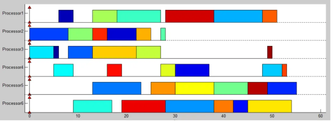
Step 5: Schedule Plot is to display the best schedule from computation, insert set of process time and start time of each job on each machine by using TORSCHE2017. The exampleof optimal

scheduling (Problem FT06) as Figure 1 which the x-axis represents Processor as Machine, for example, Processor1 means Machine1, the y-axis represents time and each color block represents

process time of each operation of each job that processes on each machine.

Figure 4: The optimal scheduling of FT06

3.3Example of output text: FT06

The program displays computation result every 10 iterations with calculated best cost (Makespan) and runtime in second as below.

(5)

Iteration 20: Best Cost = 55 t = 1.7113 Iteration 30: Best Cost = 55 t = 2.5865 Iteration 40: Best Cost = 55 t = 3.6299 Iteration 50: Best Cost = 55 t = 4.5044 Iteration 60: Best Cost = 55 t = 5.4132 Iteration 70: Best Cost = 55 t = 6.2668 Iteration 80: Best Cost = 55 t = 7.2601 Iteration 90: Best Cost = 55 t = 8.1222 Iteration 100: Best Cost = 55 t = 9.0112

This example experiment runs a problem FT06 in 100 iterations and the best solution was first found in 2 iterations within 0.2324s

4. COMPUTATIONAL RESULTS

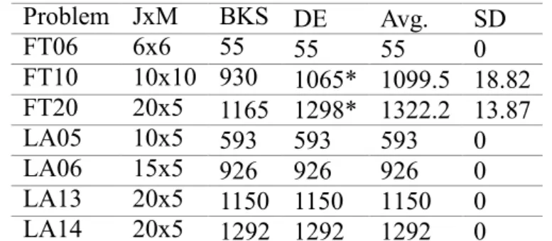
The experiments are implemented by using Matlab R2014a on the platform of Intel® Core™ i5-3230M CPU @2.60GHz with 7860 MRAM. The performance of DE is processed on selected benchmark of JSSP, test case in OR Library; FT06, FT10, FT20, LA05, LA06, LA13 and LA14, the results of computation are shown in Table 1.

Table 7: Makespan results of DE

Problem JxM BKS DE Avg. SD FT06 6x6 55 55 55 0 FT10 10x10 930 1065* 1099.5 18.82 FT20 20x5 1165 1298* 1322.2 13.87 LA05 10x5 593 593 593 0 LA06 15x5 926 926 926 0 LA13 20x5 1150 1150 1150 0 LA14 20x5 1292 1292 1292 0

The program obtains the best-known solution (BSK) in every run of 5 problems as FT06, LA05, LA06, LA13, and LA14.

*However 1065 is the best-found answer in FT10, which is 135 differ from the best-known solution and 1298 is the best-found answer in FT20, which is 133 differ from the best-known solution.

5. CONCLUSIONS

This paper is one of the experiments to solve JSSP problem by using DE approach with local move. The experimental results showed that using DE approach can solve only some small-medium size of JSSP problems with optimal solutions. However some of the medium size of JSSP problems are lost in the local optimal. So the next experiment will use additional techniques to build more effective and efficiency scheduling.

(6)

6. ACKNOWLEDGMENTS

I would like to thank Associate Professor Komkrit Leksakul and Assistant Professor Warisa Wisittipanich for their expert advice and encouragement throughout this experiment, also Associate Professor Rungchat Chompu-inwai and Associate Professor Nivit Charoenchai for their warming support as well.

This project would have been impossible without the support of the Department of Industrial Engineering, Chiang Mai University.

7. CITATIONS AND REFFERENCES

Journals: Banharnsakun, A., Sirinaovakul, B., & Achalakul, T. (2012). “Job Shop Scheduling with the Best-so-far ABC”. Engineering Applications of Artificial Intelligence, 25(3), 583-593. doi:http://dx.doi.org/10.1016/j.engappai.2011.08.003

Journals: Gonçalves, J. F., de Magalhães Mendes, J. J., & Resende, M. c. G. C. (2005). “A hybrid genetic algorithm for the job shop scheduling problem”. European Journal of Operational Research, 167(1), 77-95. doi:http://dx.doi.org/10.1016/j.ejor.2004.03.012

Journals: Gromicho, J. A. S., van Hoorn, J. J., Saldanha-da-Gama, F., & Timmer, G. T. (2012). “Solving the job-shop scheduling problem optimally by dynamic programming”. Computers & Operations Research, 39(12), 2968-2977. doi:http://dx.doi.org/10.1016/j.cor.2012.02.024 Journals: Qing, R., & Wang, Y. (2012). “A new hybrid genetic algorithm for job shop scheduling

problem”. Computers & Operations Research, 39(10), 2291-2299. doi:http://dx.doi.org/10.1016/j.cor.2011.12.005

Journals: Wisittipanich, W., & Kachitvichyanukul, V. (2011). “Two enhanced differential evolution algorithms for job shop scheduling problems”. International Journal of Production Research, 50(10), 2757-2773. doi:http://dx.doi.org/10.1080/00207543.2011.588972.