Evaluating Methods to Estimate the Implied Cost of
Equity Capital: A Simulation Study
∗
Holger Daske
†, Jörn van Halteren
‡, Ernst Maug
§December 14, 2010
Abstract
We evaluate accounting-based methods to estimate the implied cost of capital using a simulation approach. We simulate a model economy in which the true cost of capital is known and calibrate it to the CRSP-Compustat universe. We then compare the true cost of capital to the implied cost of capital estimates from ten dierent methods proposed in the literature in terms of bias, accuracy, and their correlation with the true cost of equity capital. Methods based on the residual income model perform better than those based on the abnormal earnings growth model. Methods that estimate the cost of capital and expected growth simulta-neously work reasonably well if they rely on analyst forecasts instead of ex post realized values, even if analyst forecasts are biased. We suggest combined meth-ods that are chosen so that the distortions from individual methmeth-ods compensate each other and show that some simple combinations outperform all individual methods.
JEL classications: C15, E37, M41
Keywords: Implied cost of capital, valuation, residual income, abnormal earnings growth, simulation
∗We gratefully acknowledge nancial support from the collaborative research center SFB TR
15 Governance and the Eciency of Economic Systems and the Rudolph von Bennigsen-Foerder-foundation. We thank Inessa Love, The World Bank, for sharing her STATA code to estimate vector autoregressions using panel data sets. We also thank Alon Brav, Ingolf Dittmann, Günther Gebhardt, Eva Labro, Christian Leuz, Carsten Trenkler, and workshop participants at Maastricht University, the 2nd WHU Campus for Finance, the 3rd FARS Midyear Conference San Diego, the EAA Annual Congress Istanbul, and the DGF Annual Meeting Hamburg for helpful comments and advice.
†University of Mannheim, 68131 Mannheim, Germany. E-mail: [email protected]. Tel:
+49 621 181 2280.
‡University of Mannheim, 68131 Mannheim, Germany. E-mail: [email protected].
Tel: +49 621 181 1964.
§University of Mannheim, 68131 Mannheim, Germany. E-mail: [email protected]. Tel:
1 Introduction
In this paper we evaluate accounting-based methods to estimate the implied cost of equity capital (ICC) using a simulation approach in which the true cost of capital is known. We show that ICC methods based on the residual income model perform better than those based on the abnormal earnings growth model. Combinations of several ICC methods outperform all individual methods if they average ICC estimates from rm-level calculations with estimates that simultaneously calculate the cost of equity capital and expected growth for a portfolio of rms.
Previous work has addressed the same issue based on archival data (see Easton 2009, Chapter 8 for a review). This approach faces limitations because the true cost of equity capital is unobservable, so empirical research can only compare the cost of capital from ICC methods with (1) the cost of capital generated by an asset pricing model (Lee, Ng, and Swaminathan 2009), (2) its association with other rm-specic risk characteristics (Botosan and Plumlee 2005; Brav, Lehavy, and Michaely 2005), and (3) with realized stock returns (Guay, Kothari, and Shu 2005; Easton and Monahan 2005). The rst approach encounters several well-known shortcomings outlined in the asset-pricing literature (e.g., Elton 1999; Pastor and Stambaugh 1999; Fama and French 1997, 2002). The second approach requires that the selection of the risk factors considered is correct and exhaustive, which is unlikely (Easton and Monahan 2005). The third method is based on realized returns and therefore relies on very noisy estimates (e.g., Lundblad 2007; Pastor, Sinha, and Swaminathan 2008). In the light of these limitations, it may not seem surprising that the rankings and overall evaluation of the ICC methods dier signicantly across studies.1
We perform Monte Carlo simulations of a suitably calibrated economy to address these shortcomings. Monte Carlo simulations are a well-established scientic approach, and they have been applied to address a range of questions in accounting and nance where important aspects of the underlying environment are unobservable so that tests of theories with real-world data are impossible. In simulations we observe these otherwise unknown variables by construction.2 The simulation model combines an econometric 1While research that focuses on the association of ICC methods with rm-specic risk characteristics
concludes that some ICC approaches oer reliable estimates (Botosan and Plumlee 2005), research that focuses on the association with realized returns is skeptical on the reliability of any of these estimates (Guay, Kothari, and Shu 2005; Easton and Monahan 2005; Easton 2009). See also Botosan, Plumlee, and Wen (2010) for a more cautious conclusion.
2See e.g., Greenball (1968) for a classical example, and Labro and Vanhoucke (2007, 2008) for
contemporary work. While Greenball's study is an example of studies in nancial accounting eval-1
forecasting model, a business planning model, and a DCF-based valuation model. The model parameters are calibrated to the CRSP-Compustat universe. The valuation approach is designed so that it is neutral with respect to the specic assumptions of the ICC methods and therefore creates an appropriate benchmark for comparing and analyzing these methods.
In the next step of our analysis we use ten extant ICC methods that were proposed in the literature and calculate the cost of capital these methods generate for 20,000 rms from 100 industries in our simulated economy.3 We distinguish three broad groups
of ICC methods: (1) residual income methods, which calculate the ICC individually for each rm; (2) abnormal earnings growth methods, which also determine the ICC at the rm level, and (3) industry-level methods, which estimate the cost of capital and expected growth simultaneously for a portfolio of rms.4 Finally, we compare the
ICC from these methods with the true cost of capital, which is known for each rm in our simulated economy. The evaluation of the ICC methods follows Francis, Olsson, and Oswald (2000) and applies three criteria: (1) the bias of the method, which is particularly important for the correct estimation of the equity premium (e.g., Claus and Thomas 2001); (2) the accuracy of the method, which is signicant for all practical applications of these methods, where correct rm-specic estimates of the cost of capital are required (e.g., company valuation, project appraisal); (3) the explainability of the method, which refers to the correlation between the ICC and the true cost of capital; this criterion is particularly important in research applications that require a proxy for the cost of capital.
Residual income methods have a small negative bias, whereas abnormal earnings growth methods have a larger and positive bias. Industry-level methods also tend to have a positive bias. Residual income methods tend to be the most accurate and industry-level methods that rely on analyst forecasts perform almost as well, even if uating dierent accounting methods and measurement rules (Francis 1990; Rees and Sutclie 1993; Healy, Myers, and Howe 2002), the work of Labro and Vanhoucke is representative for the management accounting literature evaluating costing systems (Lambert and Larcker 1989; Balachandran, Balakr-ishnan, and Sivaramakrishnan 1997). Other prominent areas include evaluations of alternative testing procedures commonly used in accounting research (e.g., Barth and Kallapur 1996; Kothari, Sabino, and Zach 2005), detecting audit eectiveness (e.g., Knechel 1988), or detecting earnings management (e.g., Dechow, Sloan, and Sweeney 1995).
3We use the term model for a generic modeling framework, for example the residual income model
or the dividend discount model. By contrast, we use the term method for specic methods that parameterize these models to determine the cost of capital and refer to them as ICC methods.
4We do not further divide industry-level methods, which could also be grouped into these two
categories according to the valuation model they use. 2
analyst forecasts are biased. Industry-level methods that rely on ex post realized values tend to be inaccurate, as do abnormal earnings growth methods. Residual income meth-ods also have a higher R-squared in regressions of the ICC estimates on the true cost of capital, where most industry-level methods and all abnormal earnings growth meth-ods tend to perform poorly. We attribute the generally poor performance of abnormal earnings growth methods compared to residual income methods to their modeling of future earnings. Whereas residual income methods model the level of future abnormal earnings, abnormal earnings growth methods model the changes in abnormal earnings, which seems to produce less reliable forecasts.
All methods provide distorted estimates of the cost of capital, even if the average bias is small. Firm-level methods overestimate the cost of capital if the true cost of capital is high, and underestimate the cost of capital if the true cost of capital is low. By contrast, most industry-level methods generate the opposite result. We trace this distortion to the modeling of cash ow patterns by the ICC methods by applying the concept of equity duration developed in Dechow, Sloan, and Soliman (2004) and call it the duration eect. Thus, our study contributes by adding this eect to the theoretical discussions on ICC methods in the literature (e.g., Hughes, Liu, and Liu 2009; Lambert 2009; Pastor, Sinha, and Swaminathan 2008).
Finally, we investigate the possibility that combinations of ICC methods may per-form better than individual methods.5 The analysis suggests that rm-level methods
have a lower accuracy because they systematically overestimate the true cost of capital when it is high and vice versa, whereas industry-level methods do the opposite. Com-bining methods from each category should therefore lead to better estimates because the errors of the individual methods compensate each other. We nd that this is indeed the case and we highlight two methods that combine two, respectively four, individual methods and show that they tend to outperform all individual methods as well as prior ad hoc combinations. In particular, the combination of equally weighted estimates from Gebhardt, Lee, and Swaminathan (2001) and Easton, Taylor, Shro, and Sougiannis (2002) provide a useful trade-o between simplicity and the ability to capture the true cost of equity capital in most circumstances. We conclude the paper with a number of robustness checks that highlight various aspects of our simulation model and the val-uation approach. Our main conclusions are robust to changing details of our research design.
5The general argument for combinations is based on Hail and Leuz (2006, 2009) and Dhaliwal,
A number of papers address the shortcomings of ICC methods or suggest improve-ments of existing methods. One area of improveimprove-ments is the replacement of analyst forecasts with realized values (Easton and Sommers 2007; O'Hanlon and Steele 2000) or with a statistical forecasting model (Hou, Van Dijk, and Zhang 2010). These anal-yses are complementary to ours because we derive the properties of ICC methods in a context in which unbiased forecasts are already available. Botosan and Plumlee (2005) and Easton and Monahan (2005) use dierent methodologies based on empirical data that reveal some shortcomings of existing ICC methods. By contrast, our simulation approach opens the black box, analyzes the structure of ICC methods and derives diag-nostics in an environment where the true cost of equity capital is known. On this basis we can identify the errors that are systematically built into specic methods and can then suggest combinations of methods that benet from compensating errors. Ours is not only the rst study to evaluate industry-level ICC methods, but also contributes by showing how their specic properties add to the construction of combined methods. The remainder of this paper is structured as follows. The following Section 2 de-velops the simulation approach for our model economy. We discuss the dierent ICC methods and how we implement them in Section 3. Section 4 contains the main analy-sis. In Section 5 we evaluate how the individual methods may be combined. Section 6 presents robustness checks and Section 7 concludes with a discussion of the limitations of our approach and suggestions for future research.
2 Methodology: Simulating a model economy
We conduct our simulation by setting up a business planning model, where we fore-cast a complete set of nancial statements (i.e. income statement, balance sheet, and statement of cash ows) for an economy of 20,000 rms for 50 years.6 We calibrate
the parameters of our model to those of a large sample of U.S. rms. As common in nancial modeling and corporate valuation, we use sales growth and protability (EBITDA-margin) as our main value drivers (percentage-of-sales model).7 We
empir-ically estimate the parameters that describe the joint time series of these two variables. Sales growth rates and EBITDA-margins are then the random variables in our Monte Carlo simulation from which all other accounting and cash ow items in the projected
6All calculations for this Monte Carlo simulations are implemented using MATLAB.
7We use a simplied textbook approach, see, for example, Lundholm and Sloan (2007) or Penman
nancial statements are calculated, mostly as percentages of sales. In the nal step, we draw each rm's cost of capital from a distribution and calculate the value of this rm in our simulated economy by discounting its future expected cash ows at this rate. Thus, we obtain for each rm in our simulation a complete set of nancial statements, a cost of capital, realized and expected future cash ows and earnings, and an associated rm value.
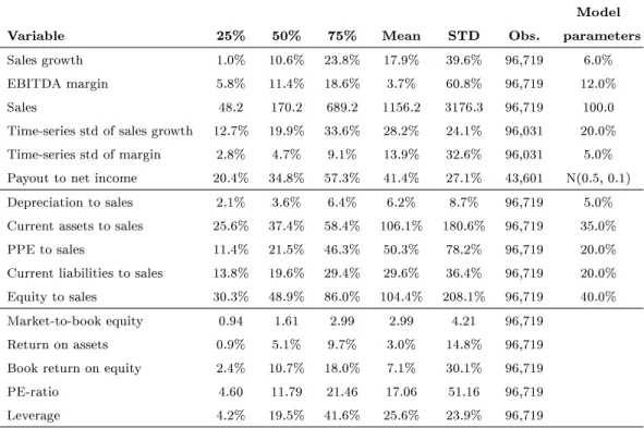
The empirical basis for calibrating our model rests on an unbalanced panel of rms from 1970 to 2009, which we obtain from the CRSP-Compustat Merged data le. We only use non-nancial rms listed on the NYSE, AMEX, or NASDAQ. We derive bal-ance sheet and income statement items from the Compustat les, while returns, divi-dends, and market capitalization are obtained from CRSP. We are left with a sample of 96,719 rm-year observations for 8,036 rms. The median rm-year in our sample has sales of $170.2 million, total assets of $154.9 million, and a market capitalization of $143.28 million (these numbers are not tabulated).
[Insert Table 1 about here.]
Table 1 summarizes the salient nancial ratios for our sample and the model pa-rameters we use for our simulation. We typically use the median of the distribution of a ratio and round the model parameters (e.g., the median ratio of property, plant and equipment to sales is 21.5%, but we use 20%). We deviate from the median rm in some instances (e.g., the plowback rate) in order to achieve a better overall calibration, particularly of the valuation ratios (PE ratio and market-to-book ratio). We provide the reason for these decisions and an assessment of the quality of our calibrations below and later perform robustness checks to show that our modeling choices are inconsequential for our main results.
2.1 Forecasting sales growth and EBITDA-margins
Vector autoregressions. We model a rm's sales growth and EBITDA margins as a rst-order vector autoregressive process (VAR(1)).8 Unlike a univariate autoregressive
(AR) model, vector autoregressions also model the cross-dependence of margins on sales growth and vice versa and therefore model also the dynamic behavior of the correlation between these key value drivers. Denote the rate of sales growth in periodt 8For a review of vector autoregressive models, see Brooks (2008). We follow the approach used in
(i.e., Salest/Salest−1 1) for rmibygSi,t and the EBITDA margin (henceforth simply:
margin) bymi,t. We then estimate the following model:9
gi,tS =α0,i+αggi,tS−1+αmmi,t−1+εi,t, (1)
mi,t =γ0,i+γggSi,t−1+γmmi,t−1 +ηi,t. (2)
We run the vector autoregression from (1) and (2) on our sample using panel VAR regression analysis. We winsorize the data for sales growth and EBITDA margins at the 1% level to reduce the impact of extreme outliers.
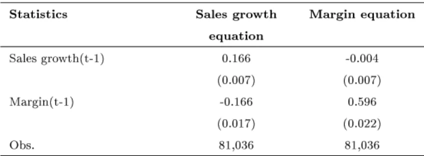
[Insert Table 2 about here.]
Panel A of Table 2 reports the results for the panel vector autoregression of sales growth and EBITDA margins. Shocks to margins exhibit some persistence (γm =
0.596), whereas the impact of sales growth on past sales growth is rather weak (αg =
0.166). There is an economically meaningful and negative impact of past margins on
sales growth (αm = −0.166). Also, there is a signicant positive correlation of 0.354
between the contemporaneous shocks to margins ηi,t and to cash ows εi,t (panel B).
We would miss these eects with univariate autoregressions. By contrast, the impact of past sales on protability is statistically insignicant (γg =−0.004).
Our rst-order VAR framework with two variables strikes a balance between sim-plicity and realism. We also experimented with second-order VAR processes, but found that second-order lags in equations (1) and (2) are only marginally signicant and gen-erate virtually identical impulse response functions. The key feature of the processes modeled here is the persistence of shocks, i.e., the length of time for which a shock to margins or sales growth has an impact on each of the value drivers. Whether the model captures the dynamic evolution of the value drivers more closely seems immaterial for valuation.
Simulations. In our Monte Carlo simulation, we generate 200 industries of 100 rms each, and for each industry we generate values for sales growth and margins from the processes (1) and (2). Ift = 0marks the beginning of our business planning model, then 9In fact, we estimate this model after rst demeaning (subtracting the time-series mean for each
variable and for each rm) and then applying a so-called Helmert transformation (see Arellano and Bover 1995, pp. 41-43, for details). As a result, we do not obtain and therefore do not report intercepts or R-squareds.
we start the processes at t = −4 because for some applications we need information
about prior periods, and we end the process att= 1 to obtain realized values for those
methods that use ex post realizations.10 We do not simulate values for periods later
thant= 1 because for later periods we only need expected values. Expected values are
always generated for 50 periods. We use the parameters from panels A and B of Table 2 with two modications.
First, we draw the beginning values at t =−4 for sales growth and for the margin
from normal distributions. The distribution of the beginning value for sales growth has a mean of 6.0% and a standard deviation of 20.0%. The median in the data from Table 1 is 10.6% for sales growth and 19.9% for the time-series standard deviation of sales growth. The mean sales growth rate of 6% in the simulations diers from the median growth rate of 10.6% in our sample (see Table 1), because we obtain better approximations for our valuation ratios for reasons we develop further below. Note that only the time-series variation and not the cross-sectional variation is relevant for calibrating the time series processes (1) and (2). The mean for the beginning value of the margin is 12% with a standard deviation of 5.0%, where the empirical values from Table 1 are 11.4% and 4.7%, respectively. We apply the same standard deviations to the residualsεi,t and ηi,t in (1) and (2) as we use for the initial values. We model these
using a joint distribution based on the empirical correlation of 0.354.
Second, we do not obtain estimates for the intercept coecientsα0 and γ0 from the panel VARs (see also footnote 9). Instead, we set these coecients so that the long-term values for sales growth and the margin from processes (1) and (2) converge to rm-specic long-term values and report the average values in panel C of Table 2. We draw long-term sales growth for each rm from a truncated normal distribution with a mean of 6% and a standard deviation of 2%. Similarly, long-term margins are drawn from a truncated normal distribution with a mean of 12% and a standard deviation of 1%. In both cases, the distribution is truncated to values within two standard deviations of the mean. Drawing long-term growth rates and margins from a distribution allows us to dierentiate between dierent types of rms, particularly growth stocks and value stocks. We obtain the interceptsα0,iandγ0,ifor our simulations by substitutingεi,t = 0,
ηi,t = 0, and the rm-specic values for long-term sales growth and the long-term margin
into equations (1) and (2) and then solving for the intercept values. For the average
10The model by Gebhardt, Lee, and Swaminathan (2001) requires information about prior periods
in order to calculate industry averages for the return on equity. Easton and Sommers (2007) use realizations of periodt= 1.
across the rm-specic intercepts we obtain α0 = 0.070 and γ0 = 0.049.
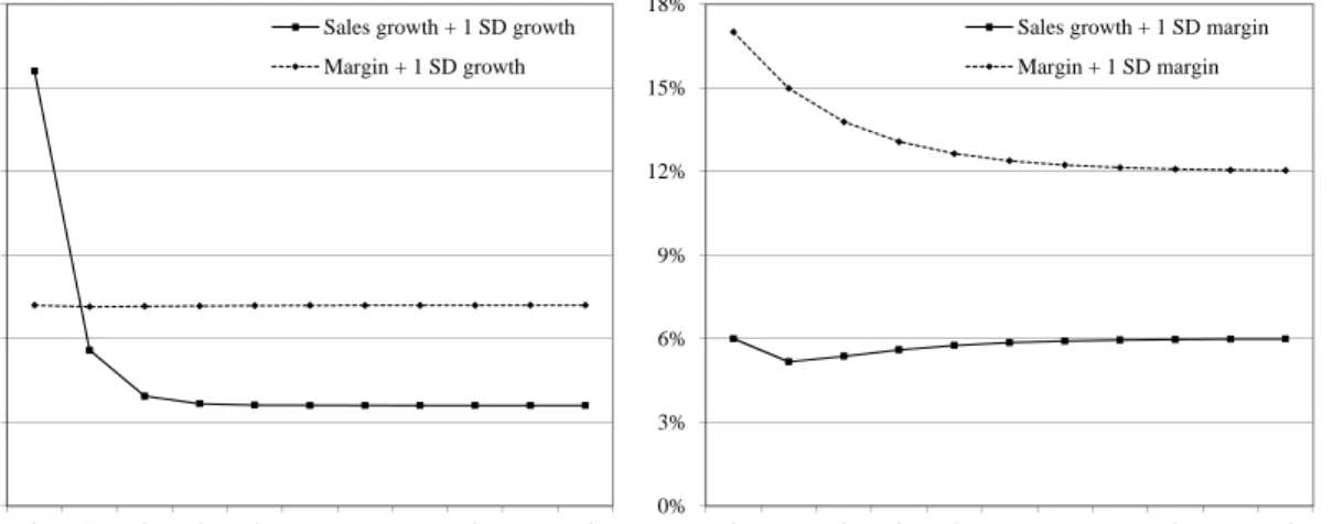
Figure 1 presents the impulse response functions of sales growth and margins for the rst 10 periods in response to a single positive, one standard deviation shock to growth (panel A) and a one standard deviation shock to the margin (panel B). We see that the processes converge relatively fast and are close to their original values after about 4 to 6 periods after the arrival of the shock if no further shocks arrive. Shocks to margins are more persistent, whereas shocks to growth have no impact on the margin. Figure 1: Impulse response functions
This gure plots the impulse response function for the sales growth and margin equations (1) and (2). The left gure shows the reactions of sales growth and margins from a one standard deviation shock (20%) to the growth rate int= 0. The right gure highlights the reactions for a one standard
deviation shock (5%) to the margin int= 0.
0% 5% 10% 15% 20% 25% 30% 0 1 2 3 4 5 6 7 8 9 10 Periods
Reaction of growth and margin to growth shocks Sales growth + 1 SD growth Margin + 1 SD growth 0% 3% 6% 9% 12% 15% 18% 0 1 2 3 4 5 6 7 8 9 10 Periods
Reaction of growth and margin to margin shocks Sales growth + 1 SD margin Margin + 1 SD margin
Forecasting and expectations. For calculating rm values and for implementing the ICC methods, we have to generate market expectations as well as analyst forecasts about future earnings and cash ows. We generate forecasts for each rm from our VAR-estimates by rst inserting the beginning values of margin and sales growth as well as the estimates for the coecients in (1) and (2) to obtain expected sales growth and margins in periodt= 1. We then use these forecasts iteratively to obtain forecasts
for period t= 2 and repeat the exercise to estimate forecasts for all periods within the
detailed planning horizon of 50 periods in our baseline simulation.
Our baseline approach assumes rational expectations. In particular, we assume that the forecasts of investors in the stock market and analyst forecasts are the same,
and that both of them use the correct model of the economy when valuing the rm. This assumption is potentially a strong one because analyst forecast bias is a widely-documented phenomenon (e.g., Brown 1993; Easton and Sommers 2007). We therefore include a robustness check where we allow for optimism on the part of analysts. Terminal values. For the terminal value after the detailed planning horizon we model terminal sales growth denoted bygi,T as a truncated normal random variable that varies
for each rm on the interval [-3%;+3%] with a mean of 0% and a standard deviation of 1%. Hence terminal growth is equal to zero on average, but not equal to zero for every rm. We later check for the impact of our terminal value assumptions by shortening or extending the detailed planning period.
2.2 Generating company values from a business planning model
Income statements. We denote expectations for sales growth and margins from our forecasting model with gˆSi,t = E(gi,tS) and mˆi,t = E(mi,t), respectively. Based on these
forecasts, we can then calculate expected sales and EBITDA from:
Si,t = (1 + ˆgi,tS)Si,t−1, (3)
EBIT DAi,t = ˆmi,t×Si,t. (4)
We set initial sales S0 to 100. We calculate depreciation as a percentage of sales and deduct it from EBITDA to obtain EBIT, and then deduct taxes at a rate of 35% of EBIT (if EBIT is positive) to obtain bottom-line net income.11 Finally, retained earnings are
equal to the plowback rate times net income; the remaining earnings are distributed as dividends. The plowback rate pb varies for each rm according to a truncated normal
distribution on the interval [0.2;0.8] with mean equal 0.5 and a standard deviation of 0.1.
Balance sheets. We construct a highly simplied balance sheet that consists only of cash, current assets (ca) and property plant, and equipment (ppe) on the assets side, and
current liabilities (cl) and shareholders' equity (book value of equity,bv) on the liabilities
and equity side. Hence, we assume that rms are fully equity nanced and abstract from debt nancing. Including interest-paying debt would require modeling the cost
of debt, debt issues, and the possibility of bankruptcy over time and would produce signicantly more complexities without generating additional results. We therefore include only current liabilities.
Current assets, net PPE, and current liabilities are all calculated as percentages of contemporaneous sales using the ratios from Table 1. The book value of equity bvt
always obeys the clean surplus condition:
bvt=bvt−1+et−dt, (5)
where et denotes total earnings (net income) and dt denotes total dividends. Cash is
the plug variable and therefore calculated as:
casht=clt+bvt−ppet−cat. (6)
Steady-state behavior. The assumptions about the model parameters, in particular the percentage-of-sales ratios, have direct implications for the long-term behavior of our business planning model. For each rm, each nancial ratio converges to some steady-state value. In the appendix we show that the return on equity converges to (denote long-term steady state values by upper bars):
roe= g
S i
pb. (7)
In our model, the return on equity therefore results from the assumptions about the plowback ratio and the long-term growth rate. In the appendix we also show that the equity-sales ratio bvt/St converges to:
bv S = 1 +g S i (m−d) (1−T)pb gSi . (8)
Given our baseline model parameters, the steady-state value of the equity-to-sales ratio from (8) equals 0.402 for the typical simulated rm, which has a plowback rate of 0.5, a long-term growth rate of 6%, and a long-term margin of 12%.
We calibrate the model so that the typical simulated rm is in a steady state, so that for this rm all nancial ratios, including the ROE and the equity-sales ratio, start out in the steady state. We therefore set the initial book valuebv0 to 40, i.e., to 40% of initial sales. For the typical simulated rm we also obtain a steady-state value of 12%
for the ROE from (7), which is equal to its starting value. However, given that the true cost of capital as well as the expected growth rates are stochastic, it is only the median rm that is in a steady state. Firms with higher growth have a higher ROE from (7) and converge to a lower equity-to-sales ratio from (8) and vice versa for low-growth rms.
Statements of cash ows. We obtain free cash ows (f cft) from earnings by adding
back depreciation (dept) and subtracting investments in working capital and capital
expenditures (changes in net PPE):
f cft=et+dept−∆Working capital−∆Net PPE
=et+dept−(cat−clt−(cat−1−clt−1))−(ppet−ppet−1+dept). (9)
Cost of capital. We draw the cost of capital from a distribution that allows us to evaluate rm-level methods as well as industry-level ICC methods and that is also consistent with the notion that growth stocks have a lower cost of capital than value stocks, thus capture the insight that the CoEC are not independent from the cash ow risks of the rm (e.g. Beaver, Kettler, and Scholes 1970). More specically, the cost of equity capitalrE,i of rm iare given by
rE,i=rE,Ind+a(¯gSi −¯g) +εi, (10)
whererE,Ind is the cost of equity capital (CoEC) of rm i's industry and g¯Si −g¯
is the deviation of rm i's long-term growth rate from the overall mean of 6%. We draw the industry cost of capital from a normal distribution with a mean of 10% and a standard deviation of 4%.12 The distribution is winsorized at the risk-free rater
f of 4.5%. Then
we draw the rm-specic component εi of the CoEC from a distribution with a mean
of zero and a standard deviation of 1%. Finally, we set a = −0.5, which generates a
dierence in mean expected equity returns between the highest book-to-market decile and the lowest book-to-market decile of 10.4% and introduces a link between cash ow shocks and shocks to expected returns. Fama and French (1992) nd return dierences between the highest and lowest book-to-market decile of around 16.7%, while Lettau and
12Easton and Monahan (2005), Table 2, report cost of equity capital in a range from 8.8% to 12.9%,
depending on the ICC method used. Other studies comparing ICC methods report only average risk premia over time, and thus do not provide a suitable direct benchmark. Dechow, Sloan, and Soliman (2004) userE= 12%to calibrate their model.
Wachter (2007) document a dierence of only 4.9%.13 We therefore use an intermediate
value in our simulation. With these parameters, the overall standard deviation of the cost of capital in our economy is thereforeq0.042+ 0.012+ (−0.5)20.022 = 0.042.
Research has identied a range of factors other than the book-to-market ratio and the value versus growth distinction that also aect the cost of capital, some for reasons that are not yet fully understood. Prominent examples are rm size, stock market liquidity, and disclosure quality.14 We abstract from these variables, which are outside
of our modeling framework. In many ways we see this aspect as an advantage of our more clinical approach. The features of the ICC methods that emerge from the simple model economy would in all likelihood also carry over to a more realistic model that would feature these additional eects. Similarly, we draw only one CoEC for each rm and assume that these CoEC do not change over time and are known to investors. The eects analyzed by Hughes, Liu, and Liu (2009) are therefore absent from our model. Equity values. We construct forecasts for all free cash ows as explained above and then calculate the market value of the equity of each rm i using the rms' drawn
cost of capital and a standard DCF-approach (e.g., Lundholm and Sloan 2007; Penman 2009). We denote these simulated rm values generated by the model byPDGP
0 , where DGP stands for data generating process:
Pi,DGP0 = 50 X t=1 E0(f cfi,t) (1 +rE,i)t + E0(f cfi,50)(1 +gi,T) (rE,i−gi,T)(1 +rE,i)50
. (11)
Our results are robust if we use the dividend discount model instead of the DCF model (11) to generate rm values.
2.3 Comparison of the simulated economy to real data
We generate 200 industries of 100 rms each using the design described in the previous two sections. For 11 out of 20,000 rms (0.1%) the market value of equity is smaller than or equal to zero.15 We classify these rms as bankrupt and remove them from 13See Fama and French (1992), Table 4, which computes a dierence of 1.4% for monthly returns,
and Lettau and Wachter (2007), Table 1.
14See Hail and Leuz (2006) for a comprehensive set of factors that inuence the CoEC empirically. 15This may happen for rms with negative current margins in combination with high cost of capital.
The negative margins generate negative free cash ows in the current periods. Later long-term positive free cash ows sometimes do not suce to outweigh the earlier negative free cash ows if the discount
further analyses.
[Insert Table 3 about here.]
Table 3 compares the simulated values with the archival data in Table 1 for key nancial ratios. For each ratio, we calculate the dierence between the quantiles for the simulated distribution and the respective quantile for the empirical distribution. We approximate the medians for sales growth, EBITDA-margin, the market-to-book ratio, and the PE-ratio very well. The market-to-book ratio is lower by 0.20 and the PE ratio is lower by 0.93 compared to the Compustat sample. The median return on assets is 2.21% higher in the simulations than the corresponding gure in our sample, whereas the median return on equity is higher in the simulations by 0.08%. Since we do not model leverage, we can only calibrate one protability ratio and therefore choose to calibrate the return on equity, which is more relevant for the valuation models. Overall, we have slightly lower valuation ratios and a higher protability in our simulated economy relative to the empirical sample. We use a plowback rate of only 50% because a higher rate leads to large book equity values and correspondingly lower market-to-book ratios. The median plowback rate of rm-years in which cash is distributed is 65% in our empirical sample (see Table 1). We show later that this decision is inconsequential for our results. Sales growth diers signicantly from the empirical data because we obtain better calibrations with a rate of 6%. This choice is realistic for two reasons. First, the empirical sample suers from survivorship bias and under represents rms with low growth rates, especially bankrupt rms. Second, growth in prots and growth in margins are closely linked in our model, but not in the data where rms also grow through zero-NPV projects like acquisitions that add to sales growth but much less to value growth.
We match the tail behavior of the empirical distribution not as accurately as the median. These dierences between the simulation and our sample come from a number of simplications. We use normal distributions throughout, whereas the distributions of the data are skewed and have tails that are dierent from those of the normal distribution (compare means and medians for key ratios in Table 1). Also, we model only the correlation between sales growth and margin in our VAR-estimations, but ignore correlations between other nancial ratios. Finally, our simulations generate values based on a typical rm with key parameters (terminal growth, plowback rate) rate is high, which then leads to market values below zero.
perturbed by random variables. Moreover, the medians in Table 1 do not correspond to a typical rm, since the median of each parameter corresponds to a dierent rm.
In summary, our simulated values are more symmetric and more concentrated around the mean than our empirical sample. To some extent these dierences are a cost we incur for the simplications we make in our simulation. The corresponding benet is that we do not need to winsorize or truncate to eliminate outliers, approaches commonly employed in empirical studies. Also, the results of our study are more rep-resentative for a typical rm. We run several robustness checks on our key modeling assumptions and show that our key results are not sensitive to the particular parameter values chosen here.
3 Implied Cost of Capital Methods
In this section we develop the ten dierent Implied Cost of Capital (ICC) methods we compare in our subsequent analysis. The starting point of all these methods is the dividend discount model (DDM), which values the equity of a rm as:
P0 = t=∞ X t=1 dt (1 +rE)t . (12)
Assuming Modigliani and Miller (1961) dividend irrelevance, the dividend discount model (12) and the DCF model (11) generate the same equity value P0.16 We
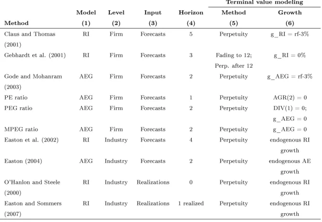
distin-guish between three groups of methods, all of which can be derived from the DDM: (1) two rm-level methods based on the residual income model, which includes Claus and Thomas (2001) and Gebhardt, Lee, and Swaminathan (2001); (2) four rm-level methods based on the abnormal earnings growth model (AEG model), which includes Gode and Mohanram (2003) and a number of methods based on capitalization ratios, which are discussed in Easton (2004); (3) four industry-level methods, which rely also on either the residual income model or on the AEG model, but estimate the cost of equity capital at the industry-level rather than at the rm level and simultaneously infer a long-term growth rate. Table 4 summarizes the key characteristics of these
16Note that our simulation model does not assume dividend irrelevance. In the model, retained
earnings generate a return that is determined by the protability implied by the EBITDA-process, which generally diers from the cost of equity of the rm.
methods.17 For all models we keep very closely to the assumptions in the respective
original articles.
[Insert Table 4 about here.]
Residual income methods. The generic equation of the residual income model can be written as: P0 =bv0+ T X t=1 aet (1 +rE)t + aeT+1 (rE −gae) (1 +rE) T, (13)
where aet denotes residual income or abnormal earnings (we use both terms
inter-changeably) at time t and gae is the long-term growth of residual income. We
imple-ment the method of Claus and Thomas (2001) (henceforth CT) by using T = 5 and gae=rf−3% = 1.5%, since we assumerf = 4.5%throughout. CT use analyst forecasts
for expected future earnings for the rst ve periods, whereas we use the forecasts of earnings from the time-series forecasts and our business planning model. As in CT, the book equity forecasts are obtained assuming a plow-back rate of 50%. The ICC is then obtained as an internal rate of return from (13).
We implement the method of Gebhardt, Lee, and Swaminathan (2001) (GLS) with
T = 12 and gae = 0. Furthermore, we can rewrite aet = (roet−rE)bvt−1, where roet
is the book return on equity. For the rst three periods we use the explicit forecasts from our forecasting model. Fromt= 3 tot = 12we use a linear interpolation between roe3 and the industry medianroe over all rms in the same industry during the last 5 years (periodst =−4 tot= 0, see above), where we exclude all rm-year observations
of rms with negative net income.
We obtain the book equity forecasts for GLS using an endogenous payout ratio, which equals the current realized payout ratio if net income is positive; otherwise the payout ratio equals current dividends divided by 6% of total assets. Also, if the esti-mated payout ratio is larger than 1 or smaller than 0, the ratio is set equal the respective boundary values. The ICC is again obtained as an IRR from (13).
17Easton (2009) provides a comprehensive survey of these methods. See also Table 1 in Easton and
Abnormal earnings growth (AEG) methods. The AEG model rests on the def-inition of abnormal earnings growth ∆aet ≡aet−aet−1:
∆aet= ∆et−rE(et−1−dt−1)
= ∆et−rE∆bvt−1, (14)
where the second line assumes the clean surplus condition. Note that the AEG model does not generally assume clean surplus, but this condition always holds in our business planning model. With the clean surplus condition imposed, the residual income model and the AEG model are isomorphic. The generic valuation equation for the AEG model is: P0 = 1 re " e1+ T−1 X t=1 ∆aet+1 (1 +rE)t + ∆aeT+1 (1 +rE) T−1 (rE−gaeg) # , (15)
which decomposes the value of equity into capitalized earnings and future earnings growth (see also Ohlson and Gao 2006).
Gode and Mohanram (2003) (GM) use T = 1 (so the middle term in (15) drops
out). Then: P0 = e1 re + ∆ae2 re(re−gaeg) , (16)
which can be rewritten as a quadratic equation. We obtain the CoEC as the larger square root of this quadratic equation. GM setgaeg =rf −3%. Dividend forecasts are
obtained using the same procedure as for the GLS method.18
Easton (2004) uses gaeg = 0, so that (16) simplies to:
P0 =
∆e2+rEd1
r2
E
. (17)
The CoEC is then obtained as rE =
p
1/MPEG, where MPEG denotes the modied
PEG ratio: MPEG=P0/(∆e2+rEd1). Similarly, with the additional assumptiond1 = 0 and the denition PEG=P0/∆e2, Easton (2004) obtains the CoEC asrE =
p
1/PEG.
Note that by construction, MPEG < PEG so that the MPEG ratio leads to a higher
estimate of the cost of capital than the PEG ratio if dividends are positive. Finally, if we assume also that ∆aet= 0 for all t ≥2, then (16) simplies to P0 =e1/rE, so that
rE = 1/PE. We implement all four applications of the AEG model in the same way,
18Note that GM use the average of the two year growth and the I/B/E/S growth rate to avoid losing
by using forecasts of dividends, earnings, and book values from our business planning model and then inferring the cost of capital according to the formulae above. Like Easton (2004) we setd1 =d0 and apply the MPEG method only to rms where∆e2 ≥0. Note from (17) that this assumption imposes a stricter condition than necessary. Industry-level methods. Industry-level methods infer the cost of capital and the growth rate simultaneously by rewriting the perpetual version of a valuation model so that it resembles a linear regression equation. We describe the approach of Easton (2004) as an example. He uses the two-period AEG model and rearranges (16) to obtain: e2 +rEd1 V0 =rE(rE −gaeg) + (1 +gaeg) e1 P0 . (18)
We run a linear regression of e2+rEd1
V0 on the forward earnings-to-price ratioe1/P0 for all
rms in the same industry. We begin by assuming a starting value of 12% for rE and
then recover one cost of capital estimate and one implied growth rate for each industry from the regression coecients in (18). We recalculate the dependent variable e2+rEd1
V0
with the values obtained and then iterate regression (18) until the estimates of the cost of equity capital and of the implied growth rate converge.19
The other portfolio approaches follow a similar logic. O'Hanlon and Steele (2000) use the residual income equation (13) withT = 1 (hence, the middle term in (13) drops
out) and obtain a regression equation with the realized book return on equityroe1 as the dependent variable. Accordingly, we implement their regression approach and use realized instead of forecasted earnings to calculateroe1.
Easton, Taylor, Shro, and Sougiannis (2002) (ETSS) start with the two-stage for-mulation of the residual income model (13) withT = 4and obtain a formulation similar
to that of O'Hanlon and Steele after aggregating earnings and dividends for the rst four years. We implement ETSS by running a linear regression of their measure of four-period cum-dividend earnings, scaled by the book value of equity, on the price-to-book ratioP0/bv0 for all rms in the same industry.
Easton and Sommers (2007) also start from the perpetual version of the residual income formula, but then assume that perpetual growth gae starts at t = 0. They
therefore obtain a regression equation in terms of roe0 instead of roe1. With this modication the implementation of their approach is similar to that of O'Hanlon and
19Convergence is achieved if both the change in the growth rate and the change in the cost of capital
Steele (2000).
4 Analysis
We start our analysis by comparing the ten individual methods for estimating the implied cost of capital. We follow Francis, Olsson, and Oswald (2000) and evaluate each method primarily in terms of its bias, accuracy, and explainability, where the latter refers to the correlation between the implied cost of capital and the true cost of capital. The importance of each of these criteria depends on the application, which we outline in the Introduction and discuss further in the Conclusion. We discuss the bias, accuracy, and feasibility in the next section 4.1 and defer the more involved analysis of explainability to Section 4.2.
4.1 Bias, accuracy, and feasibility
The starting point for each criterion is the dierence δMi ≡ rE,iM − rE,i between the
implied cost of capital rME,i estimated by method M and the true cost of capital rE,i.
Table 5 reports the results for bias and accuracy.
[Insert Table 5 about here.]
Bias. Bias is dened as the sample mean or median of δiM. For all methods except
GM and the MPEG ratio the mean and the median bias is below 2% in absolute value, which seems acceptably small. The residual income methods (CT and GLS) both slightly underestimate the cost of capital and have the lowest bias in absolute value. Three of the four methods based on the abnormal earnings growth model (GM, PEG ratio, MPEG ratio) overestimate the cost of capital, and the AEG methods have on average the largest bias in absolute value. All industry-level methods except Easton overestimate the cost of capital by about 1.1% on average.
We suspect that the rm-level methods generate biased ICC estimates because they rely on incorrect assumptions about the growth rate. Standard valuation analysis sug-gests that ICC methods should be more biased upward if they assume a growth rate that is too high. Then the upward bias in the growth rate would translate into higher model valuations, and, accordingly, a higher ICC. We analyze this point further by estimating implied long-term growth rates for each rm-level method in column (3) of
Table 5. This growth rate equates the true value of each rm with the model value given the true cost of capital. The bias in the growth rate in column (4) of Table 5 is the dierence between the implied growth rate and the growth rate assumed by the method. As expected, the biases are negative for the two residual income methods, but positive for GM. For all methods except ETSS the bias of the ICC is the same as the bias of the growth rate.
The positive bias of the three AEG methods follows from the fact that here the assumption is about the growth of abnormal earnings growth, i.e., about the growth of ∆ae, whereas the growth rate in residual income methods refers to ae itself.20 For
example, GM assumes growth of ∆ae of 1.5% per year, which implies much stronger
earnings growth and therefore a higher valuation compared to the assumption of 1.5% of the level of abnormal earnings by Claus and Thomas (see Table 4 for the model assumptions). In fact, we can have positive growth of residual income (∆aet>0) even
if abnormal earnings growth itself is constant or even negative. The negative implied growth rate of -17.4% for GM only implies that residual income will stop growing at some point, which does not rule out that it remains at a high level. A similar comment applies to MPEG, which assumes zero growth of abnormal earnings growth, which is still a much stronger assumption than the zero growth assumption of residual income made by GLS. We conclude from this discussion that the AEG methods with the standard growth assumptions in the literature are poorly calibrated.
The industry-level methods tend to display a low bias. Here the implied growth rates shown in column (3) are the growth rates predicted by these methods as part of the ICC estimation. While the bias for the implied growth rates is typically large, it does not translate one for one into a strong bias for the ICC.
Our results correspond broadly to those of Easton and Monahan (2005). We report their median ICC estimates for seven of their methods we also investigate in Table 5.21
Their ICC estimates are equal to the true CoEC, which is unknown in their setting, plus the bias of the methods. Like them, we nd the lowest ICC estimate for the PE ratio and the highest for GM, and observe that the ordering of their estimates for empirical data corresponds broadly to the ordering we obtain for simulated data.
20In some sense, g in residual income models refers to the rst derivative of the valuation function
V(g), whereas in AEG modelsg refers to the second derivative of the valuation function.
Accuracy. Accuracy refers to the typical error δM
i of the ICC estimates. We report
the median absolute value and the standard deviation of δM
i in columns (6) and (7)
of Table 5. The accuracy of ICC methods is on average low with a median absolute deviation of 2.4% and a standard deviation of 3.9% across all methods, which is large relative to a median cost of equity capital of 10%. Both measures of accuracy vary signicantly across methods, but are very consistent in terms of the implied rankings of the methods.22 Accuracy tends to be higher for the residual income methods and
for the industry-level methods, but is consistently poor for all AEG methods. CT has the highest accuracy (1.5% absolute deviation, 1.9% standard deviation), whereas the PEG ratio has the highest standard deviation (7.1%) and GM has the highest absolute deviation (3.7%).
We attribute the superiority of the residual income (RI) methods over the AEG methods to the modeling approach itself. In addition to the dierences between the methods discussed above, RI methods make use of the information contained in the book value of equity, whereas AEG methods ignore this information, which leads to larger estimation errors for the ICC. We also suspect that RI methods perform better because they use longer forecasting horizons and therefore incorporate more information. In untabulated tests we develop a two-period version of the method of Claus and Thomas, which is more comparable to the AEG methods.23 We nd that such a modied method
performs worse than the original CT method, but still outperforms all AEG methods. This observation supports the conclusion that it is the modeling approach and not just the length of the forecast horizon that explains the dierence between the results for AEG methods and for RI methods.
Among the industry-level methods, those that use realized values (O'Hanlon and Steele, Easton and Sommers) rank below those based on analyst forecasts in terms of accuracy. However, our simulation approach may exaggerate the dierence between methods based on analyst forecasts and those based on realized values because we assume rational expectations, i.e. we equate analyst forecasts with forecasts based on the correct model, an issue we address in our robustness checks. Similarly, reported earnings in practice might have more predictive ability for future earnings than in our simulated economy (e.g., by impounding managers' private information).
22We also calculate the root mean squared error (RMSE), which implies almost the same ranking of
methods as the standard deviation and is therefore not tabulated.
23We acknowledge that the AEG methods were designed to reect frequently used valuation
heuris-tics, and in particular to utilize solely the next two periods' analyst forecasts because of their frequent availability in practice. See e.g. Bradshaw (2002, 2004) and Easton (2004).
Feasibility. We note that the applicability of a method to the widest possible sample is also a quality criterion, particularly in empirical applications. Some methods cannot calculate the implied cost of capital for each rm in our sample. In particular, all two-period AEG methods can be applied only to about 61% of the rms in our model economy (column (8) of Table 5), whereas the other methods generate estimates for the cost of capital in almost all cases.24
4.2 Explainability
We analyze explainability by running simple bivariate regressions of the implied cost of capital on the true cost of capital for each method and report the estimates for the intercept and slope as well as the R-squared from these regressions in Table 6. The table shows results for OLS (columns (1) to (3)) and for median regressions (columns (4) to (6)), which are more robust to outliers. The discussion below focuses on the OLS regressions.
[Insert Table 6 here.]
R-squared. Our rst measure of explainability is the R-squared, which displays a striking variation across methods from 27% (Easton and Sommers) to 89% (Easton). Firm-specic residual income methods perform best with R-squareds of 88% (CT) and 83% (GLS), respectively. AEG methods perform worst, with R-squareds between 32% and 65% and an average of 48%. Industry-level methods are in between with an average R-squared of 56%. Methods that work with realized values (O'Hanlon and Steele, Easton and Sommers) perform poorly, as realizations seem to introduce signicant noise into cost of capital calculations. Note that the same caveat as in the case of accuracy with respect to analyst forecasts and the predictive power of realized earnings applies here as well. The ranking in terms of R-squared and the ranking in terms of median bias from Table 5 tend to agree, i.e. a higher average bias (in absolute value) tends to correspond to lower explainability in terms of R-squared.
Regression-coecient on CoEC. If the implied cost of capital methods were un-biased, then the univariate regressions should have an intercept of zero and a slope
24We restrict the algorithm to search for the implied cost of capital in the unit interval, but in a
small number of cases it can only nd solutions that are either negative or higher than 100%. In theses cases the algorithm returns a missing value.
coecient of one. Table 5 reveals that this prediction is not borne out by the data. For all rm-level methods, the intercept is negative and the estimated CoEC-coecient in the regression exceeds one signicantly. For all industry-level methods except Easton the opposite conclusion holds.
Hence, while the average bias for most methods is small, many methods still have a low accuracy because they distort the estimates for companies with true CoEC that are either very low or very high. To illustrate this point, consider the ICC estimates for GLS when the true CoEC is ve percentage points away from its mean of 10%. Then the ICC estimate is biased downward by 1.3% if the true cost of capital is only 5%, and the estimate is biased upward by 0.8% if the true cost of capital is 15%.25 By contrast,
for three of the four industry-level methods, the opposite bias obtains. For example, for ETSS we obtain a positive bias of 3.2% if the true CoEC is 5%, and a negative bias of -0.9% if the true CoEC is 15%. The eect is therefore economically large, even for those ICC methods where the average bias is small.
We label the deviation of the true CoEC from the ICC estimates distortion and refer to the regression coecient on the true CoEC as the distortion coecient. The eect diers for rm-level methods and for industry-level methods and we now investigate this phenomenon in more detail.
Distortion and the duration eect. In our model economy the DCF-value of each rm is a function of the true cost of capital: PDGP
0 = P0DGP(rE). (We suppress the
reference to the rm index for notational convenience.) Similarly, each ICC method's valuation model implies a relationship between the implied cost of equity capitalrEM and
the equity value: P0M =P0M(rME), whereM indexes the implied cost of capital methods.
Hence, the model economy and each rm-level ICC method establish a relationship
P0DGP(rE) = P0M(rME). (19)
From the implicit function theorem we then have:
drME drE = dP DGP0 (rE) drE / dP M0 (rME) drM E . (20)
The bivariate regressions in Table 6 simply estimate a linearized version of drM E
drE in (20). Hence, we obtain a large (small) slope coecient in the regressions if the sensitivity
of the rm value to the CoEC for the ICC's valuation model is smaller (larger) than the same sensitivity for the data generating process. We therefore need to understand the sensitivities dPM
0 (rME)
drM
E of rm values with respect to the cost of capital for each ICC method and for the simulation model. However, this sensitivity is nothing but the sensitivity of a present value relationship with respect to the discount rate, and we know that these sensitivities depend critically on how soon the cash ows (or earnings or dividends) are expected to arrive: The present values of cash ows that will arrive in the immediate future are not sensitive to the discount rate, whereas the present values of more distant cash ows are more sensitive. In the Appendix, we formalize this intuition by relying on the notion of equity duration developed in Dechow, Sloan, and Soliman (2004). Here we summarize the three main features of equity duration, which we denote byDU R, and defer technical details to the Appendix:
• Equity duration measures the average maturity of future cash ows (or dividends)
discounted in a present value relation. Firms whose cash ows or dividends are expected to arrive in the more distant future therefore have a larger equity dura-tion.
• Duration increases with the expected future growth rate of the rm, i.e., growth
stocks have larger equity durations compared to value stocks. This relationship is intuitive, because for faster growing rms, more of their value derives from cash ows that are expected to arrive in the distant future.
• The sensitivity of rm value with respect to the CoEC is proportional to the
equity duration of the rm. In particular, the sensitivity from (20) is given by
drEM drE
= DU R
DGP
DU RM , (21)
where DU RDGP is the equity duration implied by the data generating process,
and DU RM is the duration implied by the ICC method for the same rm. Hence, drM
E
drE is simply the ratio of the duration of the data generating process and that of the ICC method.
From the last property and the fact that DU RDGP is the same for all methods, it
follows immediately that the regression coecient on the true CoEC in Table 6 should be approximately equal to to DU RDGP/DU RM. We calculate the equity duration for
in column (7) of Table 6.26 Our tted DCF model generates a median equity duration
of DU RDGP = 18.91 years, i.e. the average cash ow in the model economy is almost
19 years away. By comparison, the median duration of the ICC methods ranges from 12.5 years (Easton) to 39.3 years (Easton and Sommers). These numbers compare to the estimate of 15 years of Dechow, Sloan, and Soliman (2004). However, their method is slightly dierent from ours and they assume a higher cost of capital.27 Based on (21)
we also calculate the ratio ofDU RDGP and DU RM for each rm and report the mean
and median of this ratio in columns (8) and (9) of Table 6.
From comparing the distortion coecients with the duration measures, and espe-cially with the mean and median of the duration ratio, in Table 6 we can observe that they are closely aligned.28 We do not expect this relationship to be perfect because
we are trying to capture the nonlinear relationship (20) with a linear regression and can safely conclude that (21) yields a very good approximation for our purposes. We can therefore attribute the pattern of distortion coecients in Table 6 to the fact that the equity duration measures implied by the rm-level ICC methods deviate from the equity duration in our tted model economy. We refer to this eect, which relates the distortion of the cost of capital to the duration of the ICC method, as the duration eect.
From the discussion above we expect that the main driver of the disparities between the equity duration of the data generating process and that of the ICC methods are the dierent assumptions about growth. From comparing the implied growth rates in Table 5 and the duration values in Table 6 we can see that there is such a relationship, although the growth rates are only available for seven methods and not strictly comparable because, as we remarked in the discussion of the bias, the growth rates of residual income cannot be compared to those of abnormal earnings growth.
In addition to the duration eect, the distortion coecient for the industry-level methods is also aected by a second feature of these methods. All industry-level meth-ods assume that growth and the cost of capital are the same for all rms within an
26We calculate the derivative dP
0/drE numerically from (28) by evaluating the average change in
the value implied by a one basis point change inrE.
27Dechow, Sloan, and Soliman (2004) calculate equity durations implied by observed stock prices
whereas we use rational forecasts of future cash ows to determine equity durations. Moreover, they assume a level perpetuity realized after ten years, which by construction leads to lower durations compared to our model with perpetual growth.
28The mean value of DU RDGP/DU RM P EG in Table 6 is distorted by one single outlier for which
the ratio exceeds 10,000. Removing this outlier leads to a value of 1.26, which is in line with the median value of 1.21.
industry, which is not the case for our simulations. As a result, the variables in the regressions suer from an errors-in-variables problem, which causes an attenuation bias for the slope coecients and leads to a reduced sensitivity of the ICC to the true CoEC.29 The bias decreases with the R-squared of the regression, which explains why
the distortion coecient and the R-squareds for the four industry-level methods are closely related and why the distortion coecient for Easton's method is above one as it also has an R-squared of 89% and therefore little attenuation bias.
Finally, we note that the distortion eect is unrelated to other factors that may inuence the cost of capital. As remarked above, our simulated economy neither features the eects of size, stock market liquidity, transparency, and other factors that may aect companies' cost of capital, nor does it model forecast bias on part of the analysts. These factors play an important role in practice and would have to be added as controls in regressions based on empirical observations.
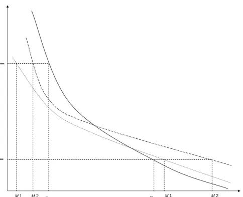
Bias and distortion. Finally, we observe that the bias of the ICC methods is closely related to the distortion coecient. The relationship between distortion and bias can be understood from Figure 2, which shows the relationship between rm value and the CoEC for the simulated values (solid line) and for two typical rm-level ICC valuation models (dotted line and dashed line). Now consider rm 1, which has a low true cost of capitalrE,1 and a high corresponding equity value P0DGP,1 , which we can read o the function for the data generating process. Firm-level ICC method M i now searches for
a cost of equity capital rM i
E,1 for rm 1 that equates this equity value with that of the model from (19). The resulting error in the cost of capital estimate is thenrE,M i1−rE,1, which is negative and equal in absolute value to the horizontal distance between the two curves. The same argument applies again to another rm 2, which has higher true cost of capital rE,2, a low equity value P0DGP,2 , and a positive error rM iE,2−rE,2. In this case,
method 1 (dotted line), which exemplies residual income methods, leads to a negative bias because the underestimation when the true cost of capital are low is much larger in absolute value than the overestimation when the true cost of capital is high. By contrast, method 2 (dashed line), which is more typical for AEG methods, leads to a positive bias because the overestimation is much larger. By experimenting with the functions for dierent methods we found that a longer forecasting horizon leads to a steeper function and therefore to a negative bias, whereas shorter forecasting horizons
29Easton (2004), Section IV discusses this problem. The attenuation bias moves the slope coecients
Figure 2: Value sensitivity for high and low value rms
This gure shows the convexity eect by illustrating the deviations arising for rms with with high versus low rm values. The graphs highlight the value sensitivities with respect to changes in the CoEC of the underlying data generating process (solid line) and two representative rm-level ICC methods (dashed and dotted lines). We plot rms' cost of equity capital on the horizontal axis and the market equity value on the vertical axis.
,1 E r 2 ,1 M E r rE,2 rEM,22 0,1 0,1 ( ) ( ) DGP E M M E P r P r 0,2 0,2 ( ) ( ) DGP E M M E P r P r 1 ,1 M E r rEM,21
lead to shallower functions and a positive bias.
5 Combining ICC methods
In the previous section we diagnose the strengths and deciencies of the ICC methods. In this section we turn to potential improvements in these methods. More specically, we consider several dierent ways of combining individual ICC methods. The rst method was suggested by Hail and Leuz (2006, 2009), who use an equally weighted average of the methods of CT, GLS, GM, and the PEG ratio. In similar spirit, Dhaliwal, Krull, and Li (2007) use the mean of CT, GLS, and GM. The third combination weights
all ten methods equally. The fourth approach applies principal component analysis and observes that the rst component captures 71% of the variation in the ICC methods.30
This observation supports the notion that the ICC methods measure one common factor. Also, the loadings of all methods on the rst principal component are positive and vary in a narrow range from 0.25 to 0.36 (these results are not tabulated).
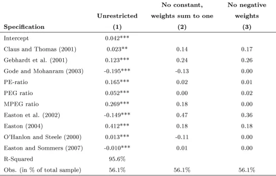
Next, we construct weights from regression analysis as follows. We run regressions of the true cost of capital rE on each of the ICC measures. The results are reported in
Table 7.
[Insert Table 7 here.]
Specication (1) is a standard OLS-regression without any restrictions. The R-squared of this regression is 95.6%, so all ten methods combined leave only 4.4% of the true cost of capital unexplained. This observation reinforces the conclusion from principal component analysis that the ICC methods jointly capture a very large part of the variation in the cost of capital. If all ICC methods were unbiased and not distorted, then any combined method should result in regression coecients that sum to one and in an intercept of zero and thereby generate the optimal weights for a combined method. However, combining the ICC measures in the way suggested by the coecients from this regression implies that the weights sum to 0.70, whereas the intercept is 0.042. Regression (2) therefore restricts the regression coecients to sum to one and sets the constant to zero. Regression (3) requires in addition that weights be non-negative. Note that several regression coecients are close to zero now, in particular all the coecients for the AEG methods, except for the industry-level method of Easton.
Finally, we consider two simple combinations that emanate from the regression analysis. Observe from regression (3) in Table 7 that only four methods are given signicant weights (CT, GLS, ETSS, and Easton) and that the weights are broadly similar. We therefore construct an equally weighted average of these four methods and label it Equally weighted - top four in the tables. Finally, we simplify even further and combine only GLS and ETSS, the best two methods, with equal weights and report it as GLS & ETSS in the tables. The reasoning for this combination is that we mainly need to remove the distortion eect in order to simultaneously improve bias, accuracy, and explainability. However, the distortion coecient from rm-level methods is above one, resulting in a negative bias, whereas the distortion coecient from industry-level
30Hail and Leuz (2009) also use principal component analysis to extract a common factor from ICC
methods is below one, resulting in a positive bias. Combining two methods, one from each category, should therefore suce to address the main shortcomings we diagnose in Section 4.
[Insert Table 8 here.]
Table 8 reports the key evaluation criteria we used in Section 4 and applies them to the combined methods. With R-squareds up to 94.3%, many ICC combinations capture a signicant portion of the true cost of capital and improve substantially relative to individual methods. Note that we have optimized the weights for the regression-based methods to match the characteristics of our simulated sample. We can therefore not legitimately compare the out-of-sample tests for ad hoc combinations with the in-sample tests for regression-based methods.
The improvement for some of the combined methods is signicant relative to the individual methods. From the in-sample methods, the weighting scheme prescribed by regression (2) performs best, with a median bias of -0.1%, a standard deviation of 1.0%, a distortion coecient of 0.99, and an R-squared of 93.6%. Hence, this method is practically unbiased and highly accurate and captures the true cost of capital almost perfectly. Specically, it outperforms the method based on unrestricted regressions, which creates signicant distortion, and the method based on principal components. However, the method based on regression (2) requires the input of all ten methods and can be computed only for the sample for which all these methods can be estimated.
From the ad hoc methods, Equally weighted - top four performs almost as well as the best regression-based method, with a bias of -0.3%, a standard deviation of 1.1%, and a distortion coecient of 1.06. This combination outperforms all other ad hoc methods as well as all individual methods. Recall that the lowest standard deviation we observe among individual methods before is for CT (1.9%, see Table 5), which then has substantially more bias and distortion. The GLS-ETSS combination performs only marginally worse on all dimensions in our economy. It provides a useful trade-o between simplicity and the ability to capture the true CoEC in most circumstances, and may therefore be recommendable for applications. By contrast, the ad hoc methods used in the prior literature (Hail and Leuz, Dahliwal et al.) perform signicantly worse, mostly because they include rm-level AEG methods, which also limits their applicability.
6 Extensions and robustness checks
All our results in the previous two sections rely on the simulated model and on the parameterization we describe in Section 2 above. In this section we check to what extent the results we report above may reect features of the simulation model rather than features of the ICC methods we wish to analyze. We want to make sure that the salient properties of the ICC methods pertain to these models and not to the simulation model.
[Insert Table 9 here.]
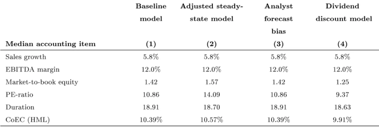
Table 9 summarizes the results for three dierent robustness checks (columns (2) to (4)). For convenience, we repeat the corresponding results for the baseline model in column (1). In panel A of the table we report the median of six key parameters for the simulated values. In the other panels we report the bias (median, panel B), accuracy (standard deviation, panel C) and explainability (distortion coecient, panel D; R-squared, panel E) for the ten individual ICC methods and for two selected combined methods.
Alternative steady state model. In Section 2.2 above we justify the simulation parameters with reference to the empirical sample, but deviate from the empirical percentage-of-sales parameters in order to better match the valuation ratios. In the alternative scenario in column (2) of Table 9 we use a parameterization that matches the empirical depreciation-to-sales ratio and the equity-to-sales ratio more closely by using 3.5% for the former (median in Compustat sample: 3.6%) and 50% for the latter (sample median: 48.9%). With these parameters the steady-state value for the equity-to-sales ratio is 48.8% from (8).
As a result, valuations for this parameterizations are somewhat higher with a market-to-book ratio of 1.57 and a PE ratio of 14.09, where the latter now exceeds the empirical median by 2.3, which renders this parameterization somewhat worse in terms of valuation. The mean bias tends to become negative, but stays about the same in absolute value. Accuracy improves for all methods, but the ranking across methods stays the same as in the baseline case. Similarly, the distortion coecient declines, but the patterns across methods is not aected. R-squareds also improve slightly. The two combined methods still improve signicantly on each of the individual methods for all