STRATEGIES FOR HIGH VACUUM DEWATERING ON PAPER MACHINES Ravi Pandey and A.K.Ray
Saharanpur Campus Department of Paper Technology Indian Institute of Technology Roorkee, India ABSTRACT
The Paper machine vacuum system is an important operation for dewatering of wet web to increase percentage solids in web. There are various models available to assess the influence of vacuum on the above parameters. In this present investigation the steady state model is discussed for estimating optimum vacuum load in flat boxes of Fourdrinier paper machine as the flat boxes are the main components to dewater the sheet in this section as well as wire and felts in the paper machine. From the detailed investigation it has been found that for a given furnish and vacuum level, there is an ultimate achievable dryness of the web beyond which the sheet will not undergo further drying , no matter what the length of exposure is. There are two main factors in vacuum dewatering - the ultimate achievable dryness for that vacuum, and the rate at which that dryness is attained. This paper also indicates the effect of temperature and slots design for vacuum dewatering.
1. Introduction
Design and optimization of papermaking vacuum system is an imperative necessity in today’s energy crisis context in a paper mill. It has been found from survey of mills of many countries including India that many machines have inadequate vacuum, with high-energy consumptions & poor operating efficiencies. According to the survey the problems are:
The vacuum levels on the wire and press section were on an average 12% higher than intended during machine design.
The measured airflow rates in the same system, through the web were 12% lower than designed.
Proper selection of vacuum system can impart potential saving in vacuum generation energy and capacity of vacuum pump, forming fabric wear, and kilowatt to overcome drag. Optimal design of vacuum level of vacuum pump system can impart potential saving in vacuum generating energy and capacity, forming fabric wear, and kiowatt to overcome drag. Unfortunately the manufacturers select the vacuum system most arbitrarily which connot be optimal in any way. It will be either over designed or under designed. The net results are excessive power consumption and quality deterioration or both. It is recognized fact that sometimes the vacuum load in suction boxes can be reduced without noticeable effect on dewatring on one side, reduction of felt and wire wear and lowering of energy consumption on the other.
To design an efficient vacuum system, it is of practical importance to understand the mechanism of the process of water removal by vacuum suction and then to implement a model- based analysis. Analysis of the model will reveal the main features of the process, the relevant mechanism, the effect of changes in the vacuum load, duration of vacuum and the thickness of the layer on the dryness (% solid content) of the layer of the web. The most critical parameters are the effects of the changes in the grammage of the layer and the duration of vacuum.
Every model requires validity and simulation which in turn demands experimental investigation of the layer and the duration of vacuum. One of the most critical parameters are the effect of the changes in the grammage of the layer and the duration of vacuum. Investigation on a commercial paper machine are not only costly, but also difficult to carry out and the results are sometimes suspected owing to the presence of uncontrollable factors. However, the results on experiments in laboratory and pilot paper maching can be used without much error for simulation purposes. Model based simulations are thus an essential tool to predict the vacuum, the optimized parameters for the vacuum producing equipments and the ancillary units.
2. Mathematical Models on vacuum dewatering
The various models of vacuum dewatering already proposed are outlined below these models are steady state or static models employing flow through porous media. These models may be static or transient. Some may be static but empirical. These are detailed below:
2.1 Static models:
(i) Darcy’s model for flow through porous media
Flow through porous media is expressed by Darcy’s law as follows;
U = - (1/µR) (dp/dw). …(1)
where, U = filtration velocity or flow rate per unit cross sectional area of the mat; µ = Viscosity of the suspending fluid;adp/dw = pressure gradient through the mat besed on grammage ;R = specific filtration resistance of the fiber mat The equation was derived for a sand cake and is valid when the fluid and porous matrix are homogenous and incompressible. Because of the compressible nature of the wet paper web, Darcy’s law connot be applied directly (5) and needs some modification. (ii) Kozeny Carman model for estimating filtration resistance
The filtration resistance given by the Kozeny Carman equation takes into account the compressibility of the material and its effect on the internal properties of the porous matrix.
R = k Sv (1-ε3 )v/ε3 …(2)
where,
ε = porosity of mat of fiber i.e. volume of voids per volume of mat.
Sv = specific surface area, i.e. surface area per unit volume of fibers
v = specific volume, i.e. volume per unit mass of fibers k= an empirical Kozeny factor
(iii) Empirical Model for displacement by compression due to Campbell(4,5)
This model was developed by Campbell, stated as displacement of fluid by compression takes place when the void fraction of medium decreases on mechanical pressing. The stiffness of the fibers and the viscous drag of the escaping fluid determine both the dynamics and the equilibrium state of the comperssion (4).
C = M Δ Pn
… … … ….(3)
where, C = consistency of fiber mat ;ΔP= pressure difference on the mat;M,n= experimentally determined constant, which depends upon the properties of the bed.
(vi) Model for channeling phenomena due to Scheidegger (13)
A serious instability, called fingering or channeling, may occur when the mobility ratio M of displacing (1) and displaced (2) fluids exceeds one.
M = (k/ μ) 1/ (k/ μ) 2 …..(4)
where, K = permeability ;μ = Viscosity
This is case in vacuum dewatering. The less viscous medium, air, is used to displace the more viscous medium, water, from the paper.
The phenomena of filtration through porous media have not been successfully applied in the paper machine vacuum dewatering.
(v) Empirical Model due to Csordas and Schiel(7)
This empirical drainage model was also develped for paper machine wet end design, using the results from very norrow (trim 25 mm) fourdrinier machine.
ΔP = [h (ex-1)/x.t]2. Q/2 ….(5)
wh ere, ΔP = p ressure d ifferen ce acro ss th e web ; h = h eigh t of th e slurry o n th e wire ; x =
empirically determined drainage index ; t = dwell time of pressure difference ; Q= drainage are (iv) Another empirical model due to Campbell ( 11)
Because of difficulty of deriving models for vacuum dewatering on the basis if know physical laws, empirical models are suggested by Campbell as under:
Q = v h (1-e-BL) …… (6)
Where, B = k (2bhp)0.5/v.f …… (6a)
q = discharge of water per wire width ;V = machine speed ;H = thickness of the web ahead of the suction box ;L = suction slit width ;f’ = web gram mage ;g = gravity constant ;hp = pressure
difference expressed as the height of the water column ;k = constant calculated after measuring water removal at the first suction box
(vi) Empirical Transcendental model due to Neun(1-3)
Neun develops an empirical model, Eq.5 which shows ‘diminishing returns’ effect in which water was progressively more difficult ot remove as the sheet become dried.
Comparisons were made between the prediction of solids and the measured solid content by experiment (using a Gamma Gauge instrument) carried out at a mill. The differences were found of the order of only from 2% to 5% points (2).
Y = b + m tanh (c. dwell). ….(7)
where, Y = solids contents obtained ;Dwell = effective suction dwell time ;m, c = parameters which control the steepness and degree of inflection of curve for the best fit ;b = a parameter wich describes the intercept of the curve at the Y – axis.
The hyperbolic tangent is truly asymptotic. 2.2 Unsteady state models
There are mainly important unsteady modelsn on vavuum dewatering are available. These are discussed below.
Tarnopolskaya et al developed a model of vacuum dewatering is based on the theory of simultanious flow of two immiscible fluids (water and air) through an unsaturated porous media. Darcy equations for water and air as well as equations of continuity for both the systems are used along with relationship for saturation and partial pressure as given u below. Detailed equations are given elsewhere(12).
Partial pressure Relationship
Pa – Pw = Pc (capillary pressure)
All the above equations are required to be scaled to identify the combinations of the parameters that define the behavior of the process. Introducing non-dimensional variables, finding suitable boundary conditions, the transformed equations are solved through asymptotic analysis numerically (8). The results indicate the saturation profiles from different vacuum loads and the effect of changes in thickness of the layer on its dryness and also the role of suction impulse. The models are verified through experimental results.
(ii) Model due to Victory(6)
Victory developed a model which has been simulated through computer regarding drainage in the forming section of the paper machine using fourdrinier wires. The mathematical model composed of three differential equations is derived from the forces acting on a differential element of the slurry as it travels on the forming medium (flow of the slurry through the mat), the vacuum created in the nip of the table rolls, and the deflection of the forming medium due to thin vacuum (6). The details of the system of equations are available elsewhere( 6,12). The problem is solved iteratiely with seven steps. These models are giving the basic behavior of the vacuum dewatering for different conditions. The model of Neun found suitable for analyzing the vacuum dewatering with medium & high speed machines.
2.3. Models for Power consumption
Typically over a half of the power needed to drive a foudrinier is caused by flat box drag. This drag also has large implications for fabric life. The vacuum and air flow used by flat boxes require substantial energy and large, costly equipment.
A method of predicting total fourdrinier load as normal running load (NRL) has been proposed by Derrick(9). For just flat boxes,the follwing equation can be used (9):
NRL = 0.0015ì (box width) (vacuum level) … ….(8)
NRL is hwrsepower/inchwidth/100fpm. ì is the coefficient of friction of the box cover; box width is the machine direction width of the box in inches, and the vacuum in inches of Hg. The cover on this machine was all made of aluminium oxide. Coefficient of friction for this material is 0.12.
3. Experimental Data of Neun
Neun develops a model which shows ‘diminishing returns’ effect in which water was progressively more difficult to remove as the sheet become drier (2).
This equaiton is based on this assumption that the input solids in the web are always more than 6%.
The ranges fo input variables are found by regression. The ranges of variables are shown here under in Table 1:
Variable Low Middle High
Solids before box,% 6 --- 12
Box vacuum, in.(mm) 3(76.2) 6(152.4) 12 Slot width,in.(mm) 0.5(12.7) 0.625(15.875),0.75(19.05) 1 Slot width, mm. 13 16,19 25 Number of slots 1 3 9 Speed, ft/min(m/min.) 1700(518.16) --- 2500(762) Speed, m/s 8.6 --- 12.7
Fabric Single layer --- Triple layer
The exposure time o f the sheet to vacuum is only the significant factor in the determination of water removal as far as slot width, dwell time, and speed are concerned. To develop a single curve for each vacuum, it was necessary to combine data for the entering sheets at 6% -12%. The lower incoming solids were 6%. After one slot, 6% becomes (6+x1)%; after two slots, it become
(6+x1+x2)% etc., until after “n” slots, it reached (6+x1+x2+….+xn)% or 12%. Note that 12% was
nominal value of actual solids before the box ,varied about ± 1%. Adding this dwell correction to the actual dwell time for the 12% data point made it equivalent to 6% inciming solids.
3.1 Relationship between Vacuum and incoming solids combinations
After studying a numcer of equations describing curves similar to Fig 1, a curve of the type shown by equation (Eq.9) provided the best fit:
Fig. 1 Sheet solids as a function slots
Percent solids can be found out by assuming the minimun solids entering the low vacuum boxes as :
In the above equation the constants m and c control the steepnesss and degree of inflection of the curve. The constant b determines the intercept. As already indicated 6% is the lowest value of incoming solids. All data had this treatment with the same incoming solids of 6%, and each data point lent a different dwell time to the data set. Analyzing the data set provided the equation for each vacuum shown in the following table (Table 2):
Table 2: Derived Models as a function of Vacuum
Vacuum Equation
3 in. (10 kPa) % Solids = 6 + 8.18 tanh (50 dwell)
6 in. (21 kPa) % Solids = 6 + 11.20 tanh (50 dwell)
12 in. (41 kPa) % Solids = 6 + 13.25 tanh (50 dwell)
Statistical regression has been applied to determine the value of the parameters c and m using 6% incoming solids. The coefficient of regression, R2, which indicates the goodness of fit, are found to be very good. The following data in Table 3, shows that the values of the constant m with the vacuum level at constant value of c.
Table: 3 Values of the constants b and m as a function of vacuum (c = 100)
Vacuum in. Hg Vacuum kPa b m R2
3 10 5.279 7.001 0.97
6 21 4.312 11.465 0.98
12 41 5.943 15.514 0.99
It is possible to combine the 6% and 12% incoming solids data into composite data sets for a given combination of equation of above table and technique described.
3.2. Relationship among GSM and vacuum level (Dwell time)
Results based on the model (Eq. 9) at different GSM and vacuum level (dwell time) for different furnishes are important for design. Table 4 shows the values of parameters estimated from the experimental data for each vacuum and basis weight (3).
Table: 4 Values fo the constants b and m as a function of Basis Weights
Basis weight (GSM) Vacuum in. Hg. m c
127 3 6 9 12 6.8 9.8 11.0 12.2 25 30 40 50 210 3 6 12 7.0 8.0 9.0 12 17 20
The above values of parameters are extremely helpful to determine the sheet solids after the box using low vacuum if dwell time is known. Alternatively the dwell time can be estimated for experimental known values of sheet solids. As an example, 127 GSM sheet at 6% solids if exposed
to 76.2 mm (3 in.) Hg of vacuum for 0.05 seconds one get from Eq. % solids,Y = 6 + 6.8 tan h (25*0.05) equal to 11.8% solids.
4. Simulation and optimization with Indian mills
4.1. Prediction for data obtained from another mill based on Neun’s Model:
The model due to Neun gives the values of solid contents with vacuum level. However, it is dependent on the design of suction foxes. The following basic data obtained from Mill-A when subjected to the models for evaluation of design data. The suction time is calculated by the speed and width of suction slots based on the Eq. 9. Estimation of percentage solids is done based on Eq. Y = b + m tan h (c* dwell time). The followingis the example how one can proceed for the simulation.
Basic weight of paper = 120 GSM
Machine speed = 152 m/min. (2530 mm/s) Deckle size = 3800 mm
Vacuum level = 100 – 200 mm (4 to 8 in Hg) in boxes Numbrer of boxes = 4
The results obtained by simulation are as follows:
Table: 5 Simulation Results at a vacuum level of 4.75 in. Hg:
Box cover Vac. (in.Hg) m c Dwell time (s) Predicted % solids 8 slots & 16 mm width 4.75 in.Hg 8.3 27 0.0506 13.76 8 slots & 16 mm width 4.75 in.Hg 8.3 27 0.1011 14.23 8 slots & 16 mm width 4.75 in.Hg 8.3 27 0.1517 14.29 8 slots & 16 mm width 4.75 in.Hg 8.3 27 0.202 14.30
Fig.2 Simulated results at 120 GSM, at 120 mm Hg Vacuum. Table 6. Simulation Results at a vacuum level of 6.in.(152.4 mm) Hg
Box cover Vac. (in.Hg) m C Dwell time (s) Predicted % solids 8 slots & 16 mm width 6 in.Hg 9.8 30 0.0506 14.3 8 slots & 16 mm width 6 in.Hg 9.8 30 0.1011 15.75 8 slots & 16 mm width 6in.Hg 9.8 30 0.1517 15.79 8 slots & 16 mm width 6in.Hg 9.8 30 0.202 15.80 .
Fig. Simulated results at 120 GSM, at (6 in)152.4 mm Hg Vacuum
Table: 7.Simulation Results at a vacuum level of 7.7 in(195.6 mm). Hg
Fig. 2. 0 5 10 15 20
0 0.0506 Sec 0.1011 Sec 0.1517 Sec 0.202 Sec
S o lid % 0 5 10 15 20
0 0.0506 Sec 0.1011 Sec 0.1517 Sec 0.202 Sec
S
o
lid
Box cover Vac. (in.Hg) m c Dwell time (s) Predicted % solids 8 slots & 16 mm width 7.7 10.4 36 0.0506 15.859 8 slots & 16 mm width 7.7 10.4 36 0.1011 16.38 8 slots & 16 mm width 7.7 10.4 36 0.1517 16.401 8 slots & 16 mm width 7.7 10.4 36 0.202 16.41
Fig. 4. Simulated results at 120 GSM, at (7.7 in) 196 mm Hg Vacuum.
From above three tables, we can predict the solids % based on different vacuum level and grades. The difference of mill data and model predicted solids contents are significant. At 3in. Hg, 6in. Hg, 9in.Hg. the maximum solids by model analysis are found to be 14.0%, 16.8%, and 18.4% respectively. In mill practice,generally the vacuum level varies from 4.7 to 7.7 in. Hg. This gave maximum level of solids between 14.30 to 16.41% respectively.
The reasons for the differences are due to
• Machine speed differences i.e. mill machine is running at low speed with different vacuum level.
• Design difference of suction box i.e. small suction slots width and the small width of box.
• Difference in the number of slots on the suction boxes i.e. more slots will maintain high flow rate of air as same as solids.
Discussion of the results
The above two ranges of vacuum level are showing that the solids content after a certain level is not increasing with vacuum level and dwell time. The third vacuum is indicating the maximum solids contents on machine.
5. Optimization with given vacuum system
0 5 10 15 20
0 0.0506 Sec 0.1011 Sec 0.1517 Sec 0.202 Sec
SO
L
ID
The optimization can be carried out by comparing different configurations of vacuum system in the wet end of paper machine. For this purpose one has to do the estimation of power for vacuum generation as well as drag load and the airflow requirements for each configuration.
The graphical optimization needs a dewatering curve. In fact, the dewatering results are also very useful for examination of existing and proposed flat box installations. The curves correlating solids contents, dwell time at various vacuum levels can predict the sheet solids after boxes at (4.75, 6, and 7.7 in.) Hg or other vacuum levels by interpolation. The % solids with the dwell time are shown below for first vacuum load.
Fig. 5 % solids as a function of dwell time.
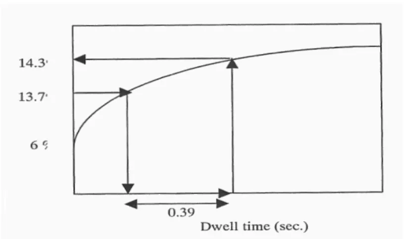
For the solids before a box of other than 6%, it is possible to use the curves as Fig. 5 illustrates. The solid content before the box is on the vertical axis with identification of the corresponding point on the curve. Calculating the dwell time of the box provides the point “up” the curve a distance of that dwell time on the horizontal axis. The corresponding solids, 4.75 in. vacuum and 8 slots of 0.75 in. width on a machine running at 152 mpm. The slots and speed yield a dwell time of 0.39 s, and outgoing solids from the curve is found as 14.3%.
A Fourdrinier machine is considered as an example with a high vacuum section with eight slots and each having 0.75 in. width and 120 GSM kraft fiber matrix. The vacuum levels in the boxes are fixed in inches Hg at 2 , 4,7 and 8 Hg consecutively. In addition, the sheet solids contents before the first box are 6%. “Stacking up” the boxes, i.e. using the output of the input of the next, provides the performance of each box. Table 8 shows the output of each box. Using the model due to Derrick (Eq. 8), one can calculate the wire drag load of the flat box section.
Table 8: Output Values from Each Box Box no. Original in. box (%solids) Dryness after box (%solids) Optimized in. box (%solids) Dryness after box (%solids) 0 --- 6 --- 6 1 7.7 15.8 0 6 2 7.7 16.3 4.7 14.3 3 7.7 16.401 6 15.8 4 7.7 16.41 7.7 16.4
The output of the flat boxes is 16.4% solids. Table lists a second set of vacuum and outputs for the flat boxes described. For this sheet, one can shut off the first box and substantially reduce other vacuum without sacrificing dryness. The calculated drag reduces to 248kW (333 hp). By this change one can reduce the drag with a saving of 25%. The calculated value of horsepower may not be exact, but it is quite probablethat drive load substantially reduces.Inherent in the drag saving is reductyion in wire wear. However,the coefficient of friction has been taken in the calculation as 0.12, which is applicable for a mid –range ceramic surface such as aluminium oxide.
Fig.-6 Percent solids after each box vs. number of boxes
Fig.6 is a plot of the dryness after each box for the two configurations. The solid line is dewatering with the original configuration. The dotted line represents curve for optimization profiles. Much less power to generate vacuum is necessary for the second configuration. Using the airflow results described above, the original configuration requires (970 ft3/ min). The optimized configuration requires (650 ft3/ min). Thus there is a potential saving due to both vacuum generation and air flow savings.
6. Conclusion and Future work:
For a given furnish and vacuum level, there is an ultimate achievable dryness beyond which the sheet will not go further dry, no matter what the length of exposure is. Therefore, two main factors in vacuum dewatering are the ultimate achievable dryness for that vacuum, and the rate at which that dryness is attained.
There were also other key findings from studies of model as given below:
1. Drive load can be optimized for significant saving, using relationships between flat box configurations and vacuum.
2. The number of slots, slots width, and speed affect dewatering only as they determine the amount of time that the sheet is exposed to vacuum (dwell time). In other words, a single one-inch slot dewaters exactly the same as two one-half-inch slots.
3. Dewatering is not a reason to change slot widths, as dwell time is unaffected.
4. Machine performance can be optimized for wire wear and vacuum use as well as sheet dryness through an understanding of the dewatering curves. This requires design of flat
S o li d s % af ter each b o x Box no. (1,2,3,4)
box configurations, which differ from industry to industry. However optimization to capitalize on potential savings in operation using reduced drive load, wire wear, and vacuum. Capital savings can also result from more frugally sized flat box sections.
More work is necessary to extend the procedure for many other paper grades, with varying furnishes and for paper with different basis weights made from same furnishes. Detailed experimental work is necessary to address the effect of other parameters like reefing temperature, air flow, steam box etc. on sheet dryness.
RERERENCES
1. Neun, J.A., 1994 TAPPI Papermaker’s conference Proceedings, pp 307 -312. 2. Neun J.A., Tappi Journal, Vol. 9:77, p.133-138 September 1994.
3. J.A. Neun, Proceedings of TAPPI papermakers conference 1995, p 259-265
4. Campbell, W.B., Lodge, W.C. Pulp and Paper Magazine of Canada 38 (1937):c, pp. 189-200
5. Campbell, W.B. Pulp and Paper Magazine Canada 48 (1947):3,pp. 103-122 6. victory E.L., Tappi J (July), vol. 52 (7), 1969, pp. 1309-1316
7. Csordas and Schiel, C: An empirical drainage model. Proceedings of the CPPA Annual meeting 1977, Montreal, pp. 151-157.
8. Pappalardo Jeff, Tappi Engineering Proceedings- “Paper Machine Vacuum System”, pp. 251-259, 1994
9. Derrick R.P., “Drive power requirements for Fourdrinier type formers”, Initial report CA#4448, TAPPI.
10.Tarnopolskaya et al., APPITA J. July 1999. pp. 275-283.
11.Campbell, W.B., Lodge, W.C., Pulp and Paper Magazine of Canada 38(1937):c, pp. 189-200
12. Pandey Ravi ,Modelling, simulations and design aspects of paper machine flat box vacuum system, 2003 – 04
13. Scheidegger, A.E., “The physics of flow through porous media”. The Macmillan Company, New York, 1960