Populations of Models, Experimental Designs and Coverage of Parameter Space by Latin Hypercube and Orthogonal Sampling

(1)

Populations of models, Experimental Designs and coverage

of parameter space by Latin Hypercube and Orthogonal

Sampling

Kevin Burrage

1,2,4

_{, Pamela Burrage}

2,4

_{, Diane Donovan}

3

_{, and}

Bevan Thompson

3∗

1 _{Department of Computer Science, University of Oxford, UK; Mathematical Sciences, Queensland}

University of Technology, Queensland 4072, Australia.

[email protected]

2 _{Mathematical Sciences, Queensland University of Technology, Queensland 4072, Australia.}

[email protected]

3 _{School of Mathematics and Physics, The University of Queensland, Queensland 4072, Australia.}

[email protected], [email protected]

4 _{ACEMS, ARC Centre of Excellence for Mathematical and Statistical Frontiers, Queensland}

University of Technology, Queensland 4072, Australia.

Abstract

In this paper we have used simulations to make a conjecture about the coverage of at dimen-sional subspace of addimensional parameter space of sizenwhen performingktrials of Latin Hypercube sampling. This takes the formP(k, n, d, t) = 1−e−k/nt−1_{. We suggest that this}

coverage formula is independent ofdand this allows us to make connections between building Populations of Models and Experimental Designs. We also show that Orthogonal sampling is superior to Latin Hypercube sampling in terms of allowing a more uniform coverage of the t

dimensional subspace at the sub-block size level. These ideas have particular relevance when attempting to perform uncertainty quantiﬁcation and sensitivity analyses.

Keywords: Population of Models, Latin Hypercube sampling, Orthogonal sampling

1 Introduction

Mathematical models are frequently highly tuned with parameters being given to many decimal places. These parameters are often ﬁtted to a set of mean observational/experimental data and so the inherent variability in the underlying dynamical processes is not captured. A very recent approach for capturing this important and intrinsic variability is based around the concept of

∗_{Authors 3 and 4 wish to thank The University of Queensland’s Centre for Coal Seam Gas (CCSG) for their}

support.

Volume 51, 2015, Pages 1762–1771

ICCS 2015 International Conference On Computational Science

1762 Selection and peer-review under responsibility of the Scientiﬁc Programme Committee of ICCS 2015

c

(2)

a population of models (POMs) [10] in which a mathematical model is built that has a set of points, rather than a single point, in parameter space, all of which are selected to ﬁt a set of experimental/observational data.

Since first proposing the POM approach for neuroscience modelling, it has been extended to cardiac electrophysiology [1], [15]. In that setting, biomarkers, such as Action Potential Duration and beat-to-beat variability, are extracted from time course profiles and then the models are calibrated against these biomarkers. Upper and lower values of each biomarker as observed in the experimental data are used to guarantee that estimates of variability are within biological ranges for any model to be included in the population. If the data cannot be characterised by a set of biomarkers then time course profiles can be used and a normalised root-mean-square (NRMS) comparison between the data values and the simulation values at a set of time points can be used to calibrate the population.

This approach suggests a possible new way in which science is done. Firstly, the POM approach leads to methodologies that are essentially probabilistic in nature. Secondly, it gives greater weight to the experimentation, modelling, simulation feedback paradigm [5]. By imple-menting experiments based on a population of models, as distinct from experiments based on a single model, the variability in the underlying structure can be captured by allowing changes in the parameters values. Such an approach avoids complications arising from decisions on the use of “best” or “mean” data, and the diﬃculties of identifying such data.

Building populations of models requires the generation of a number of parameter sets for the initial population, sampled from a possibly high-dimensional parameter space. With recent ad-vances in computational power, it is possible to generate large numbers of such models, leading to a better understanding of the systems under investigation. There are many ways to sample the parameter space, depending on costing constraints and therefore limits of computation. A parameter sweep will cover the whole parameter space at a certain discrete resolution, while random sampling, Latin Hypercube sampling (LHS) and Orthogonal sampling (OS) will give increasingly improved coverage of parameter space when the number of samples is ﬁxed and independent of the dimension of the space.

In this paper we focus on LHS, a technique ﬁrst introduced by McKay, Beckman and Conover [12]. Suppose that theddimensional parameter space is divided intonequally sized subdivisions in each dimension. A Latin Hypercube (LH) trial is a set of nrandom samples with one from each subdivision; that is, each sample is the only one in each axis-aligned hyperplane containing it. McKay, Beckman and Conover suggested that the advantage of LHS is that the values for each dimension are fully stratiﬁed, while Stein [13] showed that with LHS there is a form of variance reduction compared with uniform random sampling. A variant of LHS, known as Orthogonal sampling, adds the requirement that the entire sample space must be sampled evenly.

Depending on the underlying application, POMs may be constructed in a number of diﬀerent ways. In [1], [15], for example, POMs are developed from LHS, a useful approach because it provides insights into the nature of variability in cardiac electrophysiology. In this case the coverage of parameter space, as long as it is random in some appropriate manner, is less of an issue than for the case where POMs are used for parameter ﬁtting. In this setting, POMs have similarities with Approximate Bayesian Computation (ABC) [7]. By contrast, in ABC the sampling is usually performed adaptively so as to converge to subregions of parameter space where the calibrated models lie, as distinct from random sampling of the entire space. Thus in certain circumstances, it is important to estimate the expected coverage of parameter space givenk Latin Hypercube trials ofd-dimension.

(3)

parameter space for a population ofkLH trials with each trial of sizen. In particular, counting arguments were used to predict the expected coverage of points in the parameter space afterk

trials. These estimates were compared against numerical results based on a MATLAB imple-mentation of 100 simulations. The results of the simulations led the authors to conjecture that the expected percentage coverage byk trials of a 2-dimensional parameter space, over values

1,2, . . . , n, tended to 1−e−k/n.

As McKay, Beckman and Conover [12] state an advantage of LHS is that it stratifies each univariate mean simultaneously. Tang [14] and others have suggested that it may also be important to stratify the bivariate margins. For instance, an experimental design may involve a large number of variables, but in reality only a relatively small number of these variables are virtually effective. One way of dealing with this problem has been to project the factors onto a subspace spanned by the effective variables. However this can result in a replication of sample points within the effective subspace. Welch et al. [16] suggest LHS as a method for screening for effective factors, but Tang notes there is still no guarantee, even in the case of bivariate margins, that this projection is uniformly distributed. Thus as an alternative, Tang [14] advocates Orthogonal sampling and proposes a technique based on the existence of orthogonal arrays. He goes on to show that Orthogonal sampling achieves uniformity on small dimensional margins and further that there is a form of variance reduction. Tang’s approach is to start with an orthogonal array (defined in Section 2) and to replace its entries by random permutations to obtain an Orthogonal sample. We will expand on this idea in Section 2, as well as describing an alternate method for Orthogonal sampling.

Orthogonal arrays and covering arrays have been used also for generating interaction test suites for the testing of component-based systems. It is recognised that for large systems exhaus-tive testing may not be feasible, and instead suites are designed to test fort-way interactions,

fort= 2, . . . ,6; for details see [3], [9]. In [2] and [3], Bryce and Colbourn give a density based

greedy algorithm for the generation of covering arrays for testingt ≥2 interactions. This re-search and that in [5] have led us to investigate the relationship between Experimental Design and building POMs.

Thus in this paper rather than focusing solely on the coverage of thed-dimensional parameter space we wish to investigate the coverage of these lower dimensional subspaces. The motivation for this is that resource constraints restricting the size of the population of models may preclude significant coverage of the entire parameter space. However, it may be desirable to know if such a population of models calibrates for interactions of “small strength” by checking for all possible combinations of levels for, say, pairs or triples of variables. This would equate to investigating the coverage of two and three dimensional subspaces. The justification is that statistical techniques may be used to compare results for pairwise or three-way interactions. We will approach this question through the use of both LHS and OS. Finally, we note that the ideas discussed here are particularly relevant to both uncertainty quantification and sensitivity analysis. For example, McKay [11] and Hilton and Davis [8] give nice discussions on various aspects of uncertainty quantification and variance reduction including the need for higher order terms in any variance approximation and the role of LHS in this setting. They both emphasise that LHS is an appropriate sampling technique as it provides marginal stratification of the less important variables, while Orthogonal sampling (Tang [14]) provides marginal stratification for all pairs of random variables. Finally, Choi and Grandhi [6] develop efficient techniques to capture the essence of an uncertain response based on polynomial chaos expansions and LHS in which LHS is used to evaluate the coefficients of the Hermite basis that form the polynomial chaos expansion.

(4)

Tang’s construction for Orthogonal sampling and then give an alternate method for the genera-tion of Orthogonal samples. In Secgenera-tion 3 we report on MATLAB implementagenera-tions of simulagenera-tions of Latin Hypercube trials and Orthogonal sampling to test for uniform coverage of lower di-mensional subspaces. In Section 4 we discuss and summarise the results from Section 3 as well as discussing future directions.

2 Methodology: the construction of orthogonal samples

Before introducing constructions we review the well known methods used to generate Latin Hypercube samples and formalise the deﬁnitions for Orthogonal samples.

A Latin Hypercube trial generates an nby dmatrix where each column is a random per-mutation of{1,2, . . . , n}and then each row forms ad-tuple of the Latin Hypercube trial. Thus given an experiment ondvariables each taking parameter values 1,2, . . . , n, aLatin Hypercube

trialis a randomly generated subset ofnpoints from ad-dimensional parameter space satisfying the condition that the projections onto each of the 1-dimensional subspaces are permutations; so for each variable thenpoints cover all possible parameter values for the corresponding sub-space. By way of an example we taked= 3 andn= 8 giving below two Latin Hypercube trials LHS1 and LHS2. LHS1 LHS2 LHS3 OS LHS4 (1, 2, 1) (2, 3, 3) (3, 1, 2) (4, 7, 8) (5, 8, 5) (6, 5, 4) (7, 4, 6) (8, 6, 7) (1, 3, 2) (2, 4, 6) (3, 5, 3) (4, 7, 8) (5, 1, 1) (6, 2, 7) (7, 8, 4) (8, 6, 5) ((1,1), (1,2), (1,1)) ((1,2), (1,3), (1,3)) ((1,3), (1,1), (1,2)) ((1,4), (2,3), (2,4)) ((2,1), (2,4), (2,1)) ((2,2), (2,1), (1,4)) ((2,3), (1,4), (2,2)) ((2,4), (2,2), (2,3)) ((1,1), (1,3), (1,2)) ((1,2), (1,4), (2,2)) ((1,3), (2,1), (1,3)) ((1,4), (2,3), (2,4)) ((2,1), (1,1), (1,1)) ((2,2), (1,2), (2,3)) ((2,3), (2,4), (1,4)) ((2,4), (2,2), (2,1)) Formally, a Latin Hypercube trial H is said to be an Orthogonal sample (OS) if n = pd

and for each of the pd _d_{-tuple of the form (}_p

1, p2, . . . , pd), where 1≤ pi ≤p, there exists an

element of H of the form ((p1, x1),(p2, x2), . . . ,(pd, xd)), where 1 ≤ xi ≤pd−1. In the above

examples, d = 3 and n = 8 = 23 thus p = 2 and pd−1 _{= 4. So we rewrite the numbers}

1, . . . , n = 8 as 1 ∼ (1,1), 2 ∼ (1,2), 3 ∼(1,3), 4 ∼ (1,4), 5 ∼(2,1), 6 ∼ (2,2), 7 ∼(2,3)

and 8 ∼ (2,4). Using this representation we rewrite LHS1 as LHS3 and LHS2 as LHS4. Consider LHS3 and take the ﬁrst two 3-tuples ((1,1),(1,2),(1,1)) and ((1,2),(1,3),(1,3)) and project each ordered pair onto its ﬁrst coordinate; that is, ((1,1),(1,2),(1,1))−→(1,1,1) and ((1,2),(1,3),(1,3)) −→ (1,1,1). Then in the eight 3-tuples of LHS3 we see (1,1,1) twice, and so we cannot get all distinct eight 3-tuples on the set {1,2}. Therefore LHS3 is not an Orthogonal sample, however we can check that LHS4 is an Orthogonal sample.

Tang’s [14] construction for Orthogonal samples is based on the existence of orthogonal arrays. These are structures that can be generalised to covering arrays. Anorthogonal array

OA(N, d, n, t) ond factors, of strength t, over the set X ={1,2, . . . , n} is a subset of the d

-dimensional space

d times

X×X× · · · ×X with the property that the projection onto any of thed_t

t-dimensional subspace

t times

(5)

N=λnt_{. In a}_{covering array} _{the projections onto all}_t_{-dimensional subspaces cover the entire}

subspace with multiplicity at leastλ.

Tang takes a random orthogonal array and replaces each valuex, 1≤x≤n, by ann×1 vector where the entries correspond to a random permutation on the set {(x−1)λnt−1 +

1, . . . ,(x−1)λnt−1+λnt−1 = xλnt−1}. The rows of this new nt+1λ×d form the tuples of

a Latin Hypercube trial which is also an Orthogonal sample. The random orthogonal array is achieved by taking an orthogonal array and randomly permuting rows, columns and values within a column.

By contrast we have constructed d-dimensional Orthogonal samples (where variables take the values 1, . . . , n=pd_{, for some positive integer}_p_{) using the following procedure:}

PROCEDURE:

• Open anpd_×₂_d_array_A_{= [}_a₍_{i, j}_{)] and an}_pd_×_d_array_B _{= [}_b₍_{i, j}_)].

• Generate all possiblepd _d_{-tuples with entries chosen from 1}_{, . . . , p}_.

• Assign eachd-tuple to a separate row ofA. Then if (p1, p2, . . . , pd) is assigned to row i,

seta(i,2j−1) =pj, 1≤j≤d.

• For each 1≤j≤dcolumns 2j−1 and 2jare ﬁlled as follows. For each 1≤x≤p, identify all rowsisuch thata(i,2j−1) =x. Note that there arepd−1_{rows for each}_x_{. Generate a}

random permutation on the set{1, . . . , pd−1_}_{and assign these values sequentially to the} pd−1 _entries_a₍_i,₂_j_).

• For 1≤i≤pd _{and 1}_≤_j_≤_d_set_b₍_{i, j}_{) = (}_a₍_i,₂_j₋₁₎₋₁₎_p₊_a₍_i,₂_j_).

It is now easy to check thatB satisﬁes the deﬁnition of a Latin Hypercube trial and also an Orthogonal sample.

3 Simulation Analysis

In [4] we used Matlab simulations to make conjectures about the coverage of parameter space in terms of the number k of Latin Hypercube trials given the variable size n for dimension

d= 2. In this section we look at the coverage oft= 2 andt= 3 dimensional subspaces in the

d= 3,4,5 dimensional parameter space.

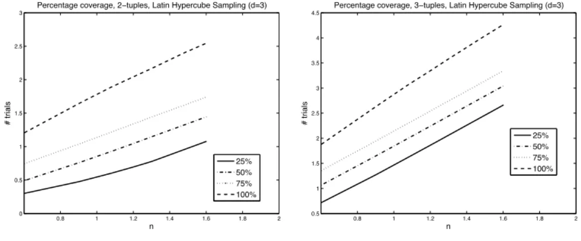
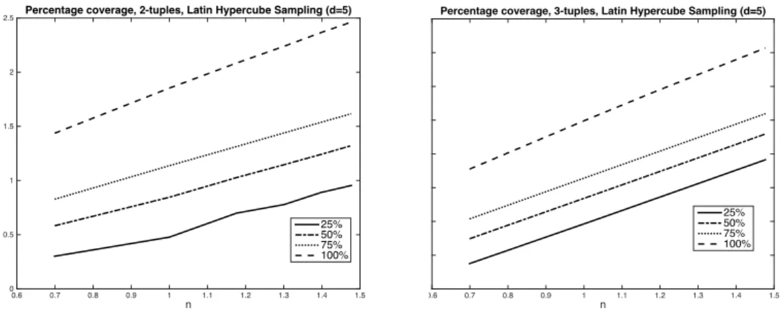
In Fig (3) we show LHS results whend= 3, for 2-tuples and 3-tuples, with coverage 25%, 50%, 75% and 100%. Fig (2) shows LHS results whend= 4, and Fig (3) gives thed= 5 results. All the quantities have been averaged over 200 trials, and the graphs plot the log₁₀of the data. When we look at the 2-dimensional subspaces (t = 2) with d = 3,4,5, we observe that the number of trials required for a speciﬁc percentage coverage is similar, regardless of the dimensiondof the system. In particular, the gradient at 25%, 50%, 75% coverage is 1, while the gradient at 100% coverage is approximately 1.25 for all values atd= 3,4,5. We observe a correspondingly similar behaviour for 3-dimensional subspaces (t= 3) ford= 3,4,5, except in these cases the gradient is 2 for incomplete coverage and approximately 2.3 for 100% coverage. In [4] we suggested that in the cased= 2 the percentage cover fork trials andndivisions is 1−e−k/n_{. The results here with} _t ₌_d _{= 3}_, _and _t ₌ _d_{= 4 suggest that when} _t ₌ _d_the

percentage coverage is given by

(6)

Figure 1: Coverage for 2-tuples (left) and 3-tuples (right), for LHS,d= 3 $"# "$ &"ï$%!#$'!"%! $"# "$ &"ï$%!#$'!"%!

Figure 2: Coverage for 2-tuples (left) and 3-tuples (right), for LHS,d= 4

$"# "$ &"ï$%!#$'!"%! $"# "$ &"ï$%!#$'!"%!

and, in the asymptotic limit askbecomes large, that it is given by

P(k, n, t, t) = 1−e−k/nt−1.

More generally we conjecture for any t < dthat

P(k, n, d, t) = 1−(1−1/nt−1)k

and, in the asymptotic limit askbecomes large, that

(7)

Figure 3: Coverage for 2-tuples (left) and 3-tuples (right), for LHS,d= 5 n 0.6 0.7 0.8 0.9 1 1.1 1.2 1.3 1.4 1.5 # trials 0 0.5 1 1.5 2

2.5 Percentage coverage, 2-tuples, Latin Hypercube Sampling (d=5)

25% 50% 75% 100% n 0.6 0.7 0.8 0.9 1 1.1 1.2 1.3 1.4 1.5

Percentage coverage, 3-tuples, Latin Hypercube Sampling (d=5)

25% 50% 75% 100%

Figure 4: Coverage for 4-tuples for LHS, ford= 4 (left) andd= 5 (right)

n 0.6 0.7 0.8 0.9 1 1.1 1.2 1.3 1.4 # trials 1.5 2 2.5 3 3.5 4 4.5

5 Percentage coverage, 4-tuples, Latin Hypercube Sampling (d=4)

25% 50% 75% 100% n 0.6 0.7 0.8 0.9 1 1.1 1.2 1.3 1.4

Percentage coverage, 4-tuples, Latin Hypercube Sampling (d=5)

25% 50% 75% 100%

This is consistent with the 25%, 50%, 75% coverage in which the gradient of the log data ist−1. The only question to address is why the gradient is slightly larger thant−1 for 100% coverage. To see this we see that 100% coverage impliesP(k, n, d, t)>1−1/nt−1_{. Thus under}

(8)

1−1/nt−1>1−(1−1/nt−1)k or

(1−p)k> p, p= 1/nt−1.

Using the fact that log(1−p)≈ −pforpsmall, then this implies

k≈(t−1) log(n)nt−1

and so

log(k)≈(t−1) log(n) + log(t−1) + log(log(n)).

It is this latter term that gives an apparent gradient slightly larger thant−1. Thus we make the following conjecture

Conjecture: The coverage of a t dimensional subspace of a d dimensional parameter space of size n when performing k trials of Latin Hypercube sampling is given by P(k, n, d, t) = 1−(1−1/nt−1₎k _{or 1}₋_e−k/nt−1 _when_k_{is large.}

Thus if costs and/or experimental factors inﬂuence the size of the sample, we can use this information to direct our experiments. So this builds conﬁdence in the modelling results.

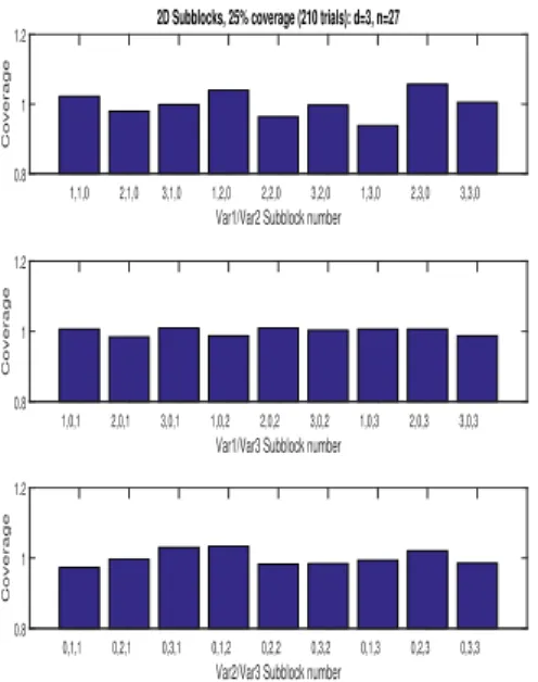
For LHS, whered= 3 andn= 27, we investigate the variability (see Fig (5)) in coverage of the sub-blocks of the 2-dimensional spaces, and compare this with Orthogonal sampling where by design the coverage is uniform over the sub-blocks.

The results in the bar graphs can be interpreted by taking a 3-dimensional parameter space, where each of the three variables takesn=pd_{= 3}3_{= 27 distinct levels. Then we partition each}

1-dimensional space intop= 3 sub-blocks of size pd−1= 9. We are interested in counting the number of points that lie in eachpd−1×pd−1sub-block when projected onto the 2-dimensional subspaces. Our simulations take the average number of Latin Hypercube trials needed to cover 25% and 75% of the parameter space and then count the number of points in each of the 2-dimensional sub-blocks. This number is taken as a fraction of the number of trials. For Orthogonal sampling this fraction is 1 across all sub-blocks but as can be seen from the ﬁgures, there is much variability when the points are generated using Latin Hypercube trials.

This emphasises the value of Orthogonal sampling versus Latin Hypercube sampling, where the latter is shown to not cover the sample space uniformly at percentage coverings that are less than 100%.

4 Conclusions

In this paper we have used simulations to give a conjecture about the coverage of atdimensional subspace of addimensional parameter space of sizenwhen performingktrials of Latin Hyper-cube sampling. This coverage takes the form P(k, n, d, t) = 1−(1−1/nt−1₎k _{or 1}₋_e−k/nt−1

whenkis large. This extends the work in [4]. We suggest that the coverage is independent ofd

and this allows us to make connections between building Populations of Models and Experimen-tal Designs. We also show that Orthogonal sampling is superior to Latin Hypercube sampling in terms of giving a more uniform coverage of the t dimensional subspace at the sub-block size level when only attempting partial coverage of this subspace. We will attempt to prove our conjecture analytically in a subsequent paper. Finally, we note that the results described here have direct relevance to uncertainty quantiﬁcation and sensitivity analyses in terms of the sampling techniques ([6]).

(9)

Figure 5: Sub-block coverage in each of the 2-dimensional subspaces for LHS with d=3, n=27, for trials giving 25% and 75% coverage.

Var1/Var2 Subblock number

1,1,0 2,1,0 3,1,0 1,2,0 2,2,0 3,2,0 1,3,0 2,3,0 3,3,0

Coverage

0.8 1

1.2 2D Subblocks, 25% coverage (210 trials): d=3, n=27

1,0,1 2,0,1 3,0,1 1,0,2 2,0,2 3,0,2 1,0,3 2,0,3 3,0,3

Coverage

0.8 1 1.2

0,1,1 0,2,1 0,3,1 0,1,2 0,2,2 0,3,2 0,1,3 0,2,3 0,3,3

Coverage

0.8 1 1.2

1,1,0 2,1,0 3,1,0 1,2,0 2,2,0 2,3,0 1,3,0 2,3,0 3,3,0

Coverage

0.8 1

1.2 2D Subblocks, 75% coverage (1010 trials): d=3, n=27

1,0,1 2,0,1 3,0,1 1,0,2 2,0,2 3,0,2 1,0,3 2,0,3 3,0,3

Coverage

0.8 1 1.2

0,1,1 0,2,1 0,3,1 0,1,2 0,2,2 0,3,2 0,1,3 0,2,3 0,3,3 Coverage 0.8 1 1.2

References

[1] O.J. Britton, A. Bueno-Orovio, K. Van Ammel, H.R. Luc, R. Towart, D.J. Gallacher, and B. Ro-driguez. Experimentally calibrated population of models predicts and explains inter subject

vari-ability in cardiac cellular electrophysiology. PNAS, 2014.

[2] R.C. Bryce and C.J. Colbourn. The density algorithm for pairwise interaction testing. Software

Testing, Veriﬁcation and Reliability, 17:159–182, 2007.

[3] R.C. Bryce and C.J. Colbourn. The density-based greedy algorithm for higher strength covering

arrays. Software Testing, Veriﬁcation and Reliability, 19:37–53, 2009.

[4] K. Burrage, P.M. Burrage, D. Donovan, T. McCourt, and H.B. Thompson. Estimates on the

coverage of parameter space using populations of models. Modelling and Simulation, IASTED,

ACTA Press, pages DOI: 10.2316/P.2014.813–013, 2014.

[5] A. Carusi, K. Burrage, and B. Rodriguez. Bridging Experiments, Models and Simulations: An

In-tegrative Approach to Validation in Computational Cardiac Electrophysiology.Am. J. Physiology,

303(2):H144–55, 2012.

[6] S-K. Choi, R.V. Gandhi, R.A. Canﬁeld, and C.L. Pettit. Polynomial Chaos expansion with Latin

Hypercube sampling for estimating response variability. AIAA Journal, 42(6):1191–1198, 2004.

[7] C.C. Drovandi, A.N. Pettitt, and M.J. Faddy. Approximate Bayesian computation using indirect

inference. Journal of the Royal Statistical Society: Series C (Applied Statistics), 60(3):317–337,

2011.

(10)

analyses of complex systems. Reliability Engineering and Systems Safety, 81:23–69, 2003. [9] D.R. Kuhn, D.R. Wallace, and A.M. Gallo. Software fault interactions and implications for software

testing. IEEE Transactions on Software Engineering, 30(6):418–421, 2004.

[10] E. Marder and A.L. Taylor. Multiple models to capture the variability of biological neurons and

networks. Computation and Systems, Nature Neuroscience, 14(2):133–138, 2011.

[11] M.D. McKay. Latin Hypercube sampling as a tool in uncertainty analysis of computer models. Proceedings of the 1992 Winter Simulation Conference, ed. J.J. Swain, D. Goldsman, R.C. Crain,

J.R. Wilson, pages 557–564, 1992.

[12] M.D. McKay, R.J. Beckman, and W.J. Conover. A comparison of three methods for selecting values

of input variables in the analysis of output from a computer code. Technometrics, 21(2):239–245,

1979.

[13] M. Stein. Large sample properties of simulations using Latin Hypercube sampling.Technometrics,

29(2):143–151, 1987.

[14] B. Tang. Orthogonal Array-Based Latin Hypercubes. Journal of the American Statistical

Associ-ation, 88(424):1392–1397, 1993.

[15] J. Walmsley, J.F. Rodriguez, G.R. Mirams, and K. Burrage; I. R. Eﬁmov; B. Rodriguez. MRNA expression levels in failing human hearts predict cellular electrophysiological remodelling: A

pop-ulation based simpop-ulation study. PLoS ONE, 8(2), 2013.

[16] W.J. Welch, R.J. Buck, J. Sacks, H.P. Wynn, T.J. Mitchell, and M.D. Morris. Screening,