NON PARAMETRIC
ROC
SUMMARY STATISTICS
Authors: M.C. Pardo
– Department of Statistics and O.R. (I), Complutense University of Madrid, 28040-Madrid, Spain
A.M. Franco-Pereira
– Department of Statistics and O.R. (I), Complutense University of Madrid, 28040-Madrid, Spain
Received: November 2015 Revised: February 2016 Accepted: April 2016
Abstract:
• Receiver operating characteristic (ROC) curves are useful statistical tools for medi-cal diagnostic testing. It has been proved its capability to assess diagnostic marker’s ability to distinguish between healthy and diseased subjects and to compare differ-ent diagnostic markers. In this paper we introduce non parametricROC summary statistics to assess a ROC curve across the entire range of F P F s∈(0,1) as well as over a restricted range ofF P F sand compare them with some existing ones through a simulation study and through some real data examples. We also show their capability to compare two diagnostic markers.
Key-Words:
1. INTRODUCTION
In a diagnostic setting, the performance of any continuous diagnostic marker is primarily assessed through the receiver operating characteristic (ROC) curve and the area under theROC curve (AU C). TheROC curve is a plot of the sen-sitivity (the probability that the marker will be above a given threshold for the diseased subjects) against 1−specificity (the specificity being the probability that the marker will be below the threshold for the healthy subjects) or, equivalently, of the true positive fraction (T P F) against false positive fraction (F P F). Using a threshold c,
ROC(·) ={(F P F(c), T P F(c)), c∈(−∞,∞)}.
The AU C is a summary measure of the sensitivity and specificity over the range of thresholds. Because of the AU C is scale free, ranging between 0.5 and 1, this measure provides a natural common scale for comparing the different markers regardless of their measurement scale. The ROC curve essentially provides a distribution-free description of the separation between the distributions of dis-eased and healthy subjects. Therefore, each of the summary measures is, in a sense, a summary of the distance between these two distributions. In fact, the empirical estimator of the AU C is equivalent to the Mann-Whitney U-statistic, thus representing the probability that a subject, randomly selected among the diseased, shows a marker value higher than a subject randomly extracted from the healthy. Other summary measure is the maximum vertical distance between the ROC curve and the 45o line, which is an indicator of how far the curve is
from that of the uninformative test. It ranges from 0 for the uninformative test to 1 for an ideal test. This index is closely related to Kolmogorov-Smirnov mea-sure of distance between two distributions ([7], [5]). Other test statistics such as Anderson-Darling, Neyman and Watson tests were studied in [16] to assess diag-nostic markers. They conclude that Anderson-Darling test is more powerful than Kolmogorov-Smirnov test and it is a good alternative to AU C. However, it can not be written in terms of functionals of the empiricalROC curve and it does not have value itself. In this paper, we propose to measure the distance between the
ROC curve and the 45oline through their derivatives to assess the discriminatory
ability of a biomarker. This approach is closely related to a nonparametric test for two sample problem based on an order statistic introduced in [1]. It does not have value itself since it is not bounded but it has a geometric interpretation in terms of the ROC curve.
When measurements on two diagnostic markers A and B are available, the question of interest is which marker best discriminates between healthy and diseased subjects. Various methods have been proposed for comparing the per-formances of two diagnostic markers. See, for example [8], [11], [19], [23] and [5]. The most commonly approach to comparing ROC curves is to test the equality
of their respectiveAU Cs. The nonparametric version of the area test was devel-oped in [9] and [10] for both unpaired and paired data. The test was refined in [6]. Two permutation tests for comparing paired ROC curves were proposed in [2] and [4]. However, when there is no uniform dominance between the involved curves, we can find different curves with the same AUC. Therefore, these tests are not valid to compare the equality among the ROC curves. In [21] it was developed a fully nonparametric test to compare twoROC curves when the data are paired and continuous. Later, [22] extended it for continuous unpaired data. In [16] it was suggested that the Anderson-Darling statistic can be viably used in comparing two diagnostic markers. Recently, [12] and [13] used the analogy between the ROC curve and the cumulative distribution function to propose a general methodology which allows us to use the traditional k-sample tests to the ROC curves comparison problem on unpaired and paired designs, respectively. Therefore, we propose, following [3], the difference between the values of our approach for each marker to compare ROC curves.
Although we focus primarily on comparing a ROC curve across the entire range of F P F s∈(0,1), in practice, one might also be interested in a part of the ROC curve that is of primary interest. For example, in screening studies,
F P F s must be kept very low and so the ROC curve over a restricted range of
F P F smay be of interest. IfF P F sin the range (0, t0) is of interest, the value of
partial ROC analysis has been recognized. [14] and [15] proposed a method for comparing a portion of ROC curves when binomial is appropriate. [24] present a nonparametric method for the analysis of partial ROC curves. Recently, [18] contruct nonparametric confidence intervals for the partial AU C. However, to our knowledge neither of the above approaches used to evaluate the whole ROC
curve based on two-sample tests, have been extended to evaluate theROC curve over a specific range. In order to fill this gap, we extend our summary statistic to evaluateROC curves over a range of F P F s of interest.
This paper is organized as follows: in Section 2 a newROC summary statis-tic which can be written as a nonparametric test based on spacings is provided as well as its partial counterpart. In Section 3 its statistical power is investigated in extensive simulations and compared with that of the standard test on AU C
and the Anderson Darling test. Furthermore, the performance of the difference of our ROC summary statistic for each marker for comparing ROC curves is studied across the entire as well as restricted range of F P F s. In Section 4 the new proposed method is applied to two real data sets. Finally, in Section 5, we make some concluding remarks.
2. THE NEW ROC SUMMARY STATISTICS
Some ROC summary measures are based on evaluating geometrically the distance between theROC curve and the 45oline, which is an indicator of how far
the curve is from that of an uninformative marker. For example, considering the area between them or the maximum vertical distance between them, we obtain the well-known AU C or the Kolmogorov-Smirnov index, respectively. However, to our knowledge, the distance between the derivatives of these two functions has not been explored as a ROC summary statistic. Therefore, our proposal is to take into account that the ROC of a noninformative marker verifies
dROC(t)
dt = lim∆t→0
ROC(t+ ∆t)−ROC(t)
∆t = 1
and to define as a summary statistic the sum of the squared differences between an approach of the derivative of the ROC curve
ROC(t)−ROC(t−N1)
1
N
, forN big enough,
and the derivative of y=x, which is 1, for a numberN of equidistant points
N X k=1 ROC(k N)−ROC( k−1 N ) 1 N −12.
In particular, we propose to considerN = 1 +nD wherenD is the number of healthy subjects and to define
η= nD+1 X k=1 ROC k nD+ 1 −ROC k−1 nD+ 1 − 1 nD+ 1 2 .
Note that the value of this summary statistic is not worthwhile by itself but it can be used to test if a biomarker is discriminatory of healthy and diseased individuals.
LetnYDi, i= 1, ..., nDo be an i.i.d. sample of a continuous distributionF
representing nD measurements of healthy subjects and let YDj, j = 1, ..., nD be an i.i.d. sample of a continuous distributionGrepresentingnD measurements
of diseased subjects. It is common in the ROC methodology to assume that diseased subjects tend to have higher measurements than healthy subjects.
The empirical estimator of the ROC curve simply applies the definition of the ROC curve to the observed data. Thus, for each possible cut-point c, the
empirical true and false positive fractions are calculated as follows: [ T P F(c) = nD P i=1 I(YDi ≥c) nD \ F P F(c) = nD P j=1 IYD j ≥c nD .
The empiricalROCcurve is a plot ofT P F[ (c) versus\F P F(c) for allc∈(−∞,∞).
Equivalently, the empiricalROC can be written as
\ ROC(t) = T P F[ \F P F−1(t), t∈(0,1). Let−∞ =YD (0) ≤YD(1) ≤YD(2) ≤...≤YD(n D) ≤YD (n D+1) =∞be the or-der statistics constructed from nYD
j, j = 1, ..., nD
o
. Therefore, an estimator of
η can be obtained replacingROC by its empirical estimator:
b η = nD+1 X k=1 \ ROC k nD+ 1 −\ROC k−1 nD+ 1 − 1 nD + 1 2 .
Note that this index is the sum of squared errors between the jump of the ROC curve evaluated in two equidistant points and the distance between these two equidistant points. The value 0 means to be a noninformative test. Furthermore, this index, ηb, is closely related to the nonparametric test for a two sample problem based on order statistics proposed in [1]. Indeed, we see that
\ ROC k nD+ 1 =T P F[ \ F P F−1 k nD+ 1
so first we look for a value v such as
\ F P F(v) = k nD+ 1 or equivalently, nD+1 X j=1 IYD j ≥v =k sov = YD (n D−k+1) .Therefore, \ ROC k nD+ 1 = nD P i=1 I YDi ≥YD(n D−k+1) nD .
In a similar way, \ ROC k−1 nD+ 1 = nD P i=1 I YDi ≥YD(n D−k+2) nD . Finally, b η = nD+1 X k=1 nD P i=1 ξi k nD − 1 nD+ 1 2 where ξki = 1, YDi ∈∆k 0, YDi ∈/ ∆k fork= 1, ...., nD+ 1, i= 1, ..., nD, with ∆k = YD (n D−k+1) , YD (n D−k+2)
, is the test statistic proposed in [1]. They obtained its exact distribution that can be seen in Theorem 1.
If F P F s in the range (0, t0) is of interest, the partial bη can be similarly
defined as (2.1) b ηp(t0) = X 1≤k≤[t0(nD+1)] nD+1 X k=1 \ ROC k nD+ 1 −\ROC k−1 nD+ 1 − 1 nD+ 1 2
where [·] denotes the integer part of·.
In the following section we evaluate the performance of ηband compare it to the ordinary nonparametric ROC test AU C[ given by
[ AU C= PnD i=1 PnD j=1I(YDi < YDj) nDnD .
and the Anderson-Darling test of uniformity of the distribution of the false posi-tive fraction, proposed in [16] (AD) to assess one diagnostic marker.
On the other hand, the test statistic
T = q AU C\A−AU C\B
var(AU C\A) +var(AU C\B)−2covar(AU C\A,AU C\B)
,
proposed by [6] and ∆Z =ZB−ZA, forZL= ˆη, AD, whereL=A, B, indicates
the value of the test statistic for biomarker A orB, are compared to assess two biomarkers. Finally, the partial summary measure ηbp(t0) is compared to the partial AU C,pAU C(t0), via bootstrap.
3. SIMULATION STUDIES
Firstly, simulations are conducted to assess the performance of the new
ROC summary statisticηb, to evaluate one marker. We have compared the power of our statistic ηbwithAU C[ and AD.
Table 1 compares the power of ηb obtained when the exact distribution studied in [1] is used to obtain the critical values and when 1,000 Monte Carlo replicates are used instead. Due to the relatively large computational time re-quired for the implementation of the exact procedure, the comparisons presented here are limited to small samples (nD =nD = 15). However, even with these
small samples, there is a good agreement between the exact and simulated test. Thus, for the large sample sizes as presented in the subsequent tables, we cal-culate only the power of the simulated test since the results for the exact test should be essentially the same.
Table 1: Comparison of the power of ηb obtained using the exact dis-tribution and the one obtained via 1,000 independent Monte Carlo simulations, fornD =nD = 15. Healthy subjects follow (from left to right) aN(0,1), Γ(1/2,1/2) orLN(0,1) distribu-tion while diseased subjects are sampled fromG.
G Exact MC G Exact MC G Exact MC
N(0.3,1) 0.074 0.074 Γ(2,1) 0.987 0.986 LN(1.275,0.5) 0.793 0.771
N(0.3,1.42) 0.133 0.119 Γ(4,1) 1.000 1.000 LN(0,3/2) 0.056 0.050
N(0.3,0.32) 0.981 0.977 Γ(4.3,4) 1.000 1.000 LN(0.7,0.2) 0.894 0.894
N(0,1.42) 0.117 0.111 Γ(1/8,1/8) 0.844 0.830 LN(−3/2,2) 0.576 0.540
N(0,0.32) 0.973 0.969 Γ(4,4) 1.000 1.000 LN(1/4,1/2) 0.279 0.258
For 1,000 independent simulations, one-sided tests were conducted at level
α = 0.05 to compare theAU C[,ADandηbtests. To determine appropriate critical values we have carried out Monte Carlo simulation with M = 5,000 replicates. The type I error values are not presented as they are all around 0.05 but they can be provided by the authors upon request. Tables 2–4 compare the proportion of rejections (power) for different pairs of distributions for diseased and healthy subjects. These three tables distinguish three different distributions for the mark-ers: Normal, Gamma and Lognormal, respectively. The markers for the healthy subjects are generated from a N(0,1), Gamma(1/2,1/2) and LN(0,1), respectively while the markers for the diseased subjects are generated from five different alter-natives each one. These alteralter-natives have been considered taking into account all the possible combinations changing the location and shape of the distribution of the diseased subjects in relation to the healthy subjects. Some of the probability
distribution functions and their corresponding ROC curves for Table 2 can be seen in Figure 1.
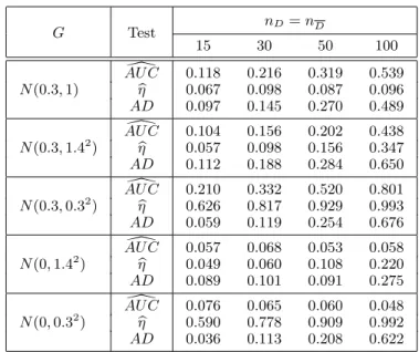
Table 2: Power based on 1,000 independent simulations of Normal ran-dom variables. Healthy subjects follow aN(0,1) distribution while diseased subjects are sampled fromG.
nD=nD G Test 15 30 50 100 [ AU C 0.118 0.216 0.319 0.539 N(0.3,1) ηb 0.067 0.098 0.087 0.096 AD 0.097 0.145 0.270 0.489 [ AU C 0.104 0.156 0.202 0.438 N(0.3,1.42) b η 0.057 0.098 0.156 0.347 AD 0.112 0.188 0.284 0.650 [ AU C 0.210 0.332 0.520 0.801 N(0.3,0.32) ηb 0.626 0.817 0.929 0.993 AD 0.059 0.119 0.254 0.676 [ AU C 0.057 0.068 0.053 0.058 N(0,1.42) b η 0.049 0.060 0.108 0.220 AD 0.089 0.101 0.091 0.275 [ AU C 0.076 0.065 0.060 0.048 N(0,0.32) b η 0.590 0.778 0.909 0.992 AD 0.036 0.113 0.208 0.622 −4 −2 0 2 4 0.0 0.2 0.4 0.6 0.8 1.0 1.2 1.4 Density −4 −2 0 2 4 0.0 0.2 0.4 0.6 0.8 1.0 1.2 1.4 Density −4 −2 0 2 4 0.0 0.2 0.4 0.6 0.8 1.0 1.2 1.4 Density FPF TPF 0.0 0.1 0.2 0.3 0.4 0.5 0.6 0.7 0.80.9 1.0 0.0 0.2 0.4 0.6 0.8 1.0 FPF TPF 0.0 0.1 0.20.3 0.4 0.5 0.6 0.7 0.8 0.9 1.0 0.0 0.2 0.4 0.6 0.8 1.0 FPF TPF 0.0 0.1 0.2 0.3 0.4 0.50.6 0.7 0.8 0.9 1.0 0.0 0.2 0.4 0.6 0.8 1.0
Figure 1: Probability distribution functions and their corresponding ROC
curves (nD =nD = 100) for some cases described in Table 2. From left to right: N(0,1) versus N(0.3,1), N(0.3,0.32) and
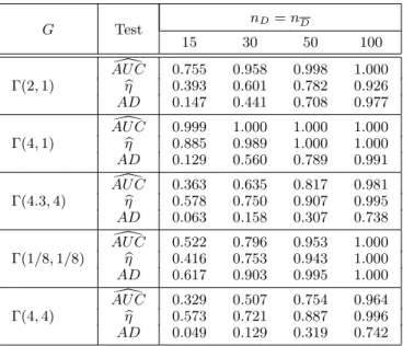
Table 3: Power based on 1,000 independent simulations of Gamma ran-dom variables. Healthy subjects follow a Γ(1/2,1/2) distribu-tion while diseased subjects are sampled fromG.
nD=nD G Test 15 30 50 100 [ AU C 0.755 0.958 0.998 1.000 Γ(2,1) ηb 0.393 0.601 0.782 0.926 AD 0.147 0.441 0.708 0.977 [ AU C 0.999 1.000 1.000 1.000 Γ(4,1) ηb 0.885 0.989 1.000 1.000 AD 0.129 0.560 0.789 0.991 [ AU C 0.363 0.635 0.817 0.981 Γ(4.3,4) ηb 0.578 0.750 0.907 0.995 AD 0.063 0.158 0.307 0.738 [ AU C 0.522 0.796 0.953 1.000 Γ(1/8,1/8) ηb 0.416 0.753 0.943 1.000 AD 0.617 0.903 0.995 1.000 [ AU C 0.329 0.507 0.754 0.964 Γ(4,4) ηb 0.573 0.721 0.887 0.996 AD 0.049 0.129 0.319 0.742
Table 4: Power based on 1,000 independent simulations of LogNormal random variables. Healthy subjects follow a LN(0,1) distri-bution while diseased subjects are sampled fromG.
nD=nD G Test 15 30 50 100 [ AU C 0.976 1.000 1.000 1.000 LN(1.275,0.5) ηb 0.734 0.946 0.995 0.999 AD 0.133 0.424 0.744 0.985 [ AU C 0.055 0.064 0.051 0.051 LN(0,3/2) ηb 0.058 0.083 0.182 0.325 AD 0.089 0.106 0.174 0.420 [ AU C 0.706 0.922 0.999 1.000 LN(0.7,0.2) ηb 0.883 0.987 1.000 1.000 AD 0.038 0.096 0.198 0.541 [ AU C 0.668 0.941 0.995 1.000 LN(−3/2,2) ηb 0.536 0.895 0.993 1.000 AD 0.711 0.976 0.999 1.000 [ AU C 0.132 0.224 0.334 0.584 LN(1/4,1/2) ηb 0.270 0.364 0.517 0.718 AD 0.067 0.159 0.283 0.688
Every table follows the same pattern: in the first three designs the mean of the diseased subjects is larger than the mean corresponding to the healthy ones and in the last two designs it does not change. In the first design, the standard
deviation of both groups of patients is the same, in the second and forth one the standard deviation of the diseased subjects is larger, and in the third and fifth one the standard deviation of the diseased subject is smaller.
As [16] already observed, these results reveal that the AU C[ test is more powerful when location differences between the distributions under consideration are primarily involved. However, in our study, although the mean increases if the standard deviation decreases (design 3) our procedure has higher power than the others. When scale differences are prominent, AU C[ test is incapable of discrim-inating between these distributions. In particular, when the standard deviation of the distribution of the healthy subjects is larger than that for the diseased subjects, the new measure ηbis significantly better than AU C[ and AD tests. If the standard deviation of the distribution of the healthy subjects is smaller than that for the diseased subjects, theADtest is preferable to the others. Therefore, our procedure is the best when the standard deviation of the distribution of the healthy subjects is larger than that for the diseased subjects independently that the location of the distribution of the diseased subjects changes or not (designs 3 and 5). These two designs as can be seen in Figure 1 correspond to ROC curves crossing the diagonal reference line. Moreover, for the other designs it is the sec-ond best except for designs 1 and 2 in Table 2. Although AU C[ test is preferable when location differences between the distributions under consideration are pri-marily involved, we must not use it in the other situations. Finally,AD test has only slight high power than our procedure in one of the five considered designs.
3.1. Assessment of two diagnostic markers
We compare the performance of our test statistic, ∆ηb, to that of [6],T, and Anderson Darling approach, ∆AD, via simulation. In [16] it was concluded that the DeLong test is in general more powerful than the Anderson-Darling approach to assess two diagnostic markers, particularly when the correlation between mea-surements is substantial. In the simulations to obtain the distributions of AD
test and our test we have used bootstrap following [3].
We perform simulations to investigate the empirical power for different un-derlying AUCs, correlations between the markers (ρ = 0,0.5) and different simple sizes (nD =nD = 20,40,80) at level α = 0.05. In these simulations, the marker
values of the healthy subjects were generated from a standard normal distribu-tion and those of the diseased subjects from N(µA, σ2A= 1) and N(µB, σB2) for
markers A and B, respectively. The uniform alternative (where one curve is uniformly above the other) occurs when σA2 =σ2B and the crossing alternative (when the two curves cross) when 4σ2
A =σ2B. For each considered scenario, 1000
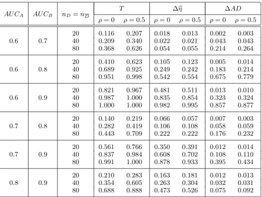
For equalAU Cs arising from crossing ROC curves, the power of our test is the highest as can be seen in Table 5 and the use of theT test is inappropriate. On the other hand, highly correlated biomarkers lead to increase power. For non-crossing ROC curves, the power of T test is the highest as can be seen in Table 6. The power of ∆ηbis higher than the power of ∆AD.
Table 5: Power against crossing alternatives.
T ∆ηb ∆AD AU CA AU CB nD=nD ρ= 0 ρ= 0.5 ρ= 0 ρ= 0.5 ρ= 0 ρ= 0.5 20 0.046 0.066 0.014 0.019 0.015 0.018 0.6 0.6 40 0.063 0.048 0.088 0.075 0.072 0.073 80 0.046 0.049 0.327 0.338 0.162 0.190 20 0.055 0.046 0.042 0.025 0.040 0.039 0.7 0.7 40 0.057 0.045 0.132 0.148 0.095 0.127 80 0.039 0.043 0.421 0.478 0.092 0.136 20 0.054 0.037 0.069 0.074 0.061 0.062 0.8 0.8 40 0.061 0.051 0.193 0.209 0.110 0.155 80 0.051 0.053 0.475 0.577 0.111 0.155 20 0.044 0.038 0.092 0.108 0.070 0.095 0.9 0.9 40 0.049 0.041 0.195 0.218 0.147 0.157 80 0.056 0.054 0.459 0.541 0.232 0.277
Table 6: Power against uniform alternatives.
T ∆ηb ∆AD AU CA AU CB nD=nD ρ= 0 ρ= 0.5 ρ= 0 ρ= 0.5 ρ= 0 ρ= 0.5 20 0.116 0.207 0.018 0.013 0.002 0.003 0.6 0.7 40 0.209 0.340 0.022 0.021 0.043 0.043 80 0.368 0.626 0.054 0.055 0.214 0.264 20 0.410 0.623 0.105 0.123 0.005 0.014 0.6 0.8 40 0.689 0.925 0.249 0.242 0.183 0.214 80 0.951 0.998 0.542 0.554 0.675 0.779 20 0.821 0.967 0.481 0.511 0.013 0.010 0.6 0.9 40 0.987 1.000 0.835 0.854 0.323 0.324 80 1.000 1.000 0.982 0.995 0.857 0.877 20 0.140 0.219 0.066 0.057 0.007 0.003 0.7 0.8 40 0.282 0.419 0.106 0.108 0.058 0.059 80 0.443 0.709 0.222 0.222 0.176 0.232 20 0.561 0.766 0.350 0.391 0.012 0.014 0.7 0.9 40 0.837 0.984 0.608 0.702 0.108 0.110 80 0.991 1.000 0.878 0.933 0.395 0.434 20 0.210 0.283 0.163 0.181 0.012 0.013 0.8 0.9 40 0.354 0.605 0.263 0.304 0.032 0.031 80 0.688 0.888 0.473 0.526 0.075 0.092
In summary, the behavior of our test is the same asAD test studied in [16] and permutation tests introduced in [21]. That is to say, they have clearly superior power in Table 5 to T test but the power of ours is the highest. However, the power of the permutation test proposed in [2] is close to the nominal significance level suggesting that a rejection of the null hypothesis is unlikely to occur. On the other hand, for non-crossing ROC curves, T test is preferable although as sample size increases the power of ∆ηbis closer to the power ofT test. Note that in most of the cases ∆AD test has very low power (see Table 6).
Finally, suppose one is only interested in some range of specificities. For example, acceptable specificities are high for early cancer detection tests. A lower specificity for a large population leads to many more falsely classified non-diseased subjects who may have to undergo a more invasive test subsequently. It is thus desired to compare screening markers at a higher range of specificities. The partial AU C, which summarizes part of the ROC curve in the range of desired specificities, uses to be a better alternative to T test. The value of partial
ROC analysis has been recognized and several methods have been developed. See [14], [15], [20] and [17]. However, the methods for analysing partial ROC presented in these papers use a parametric approach which assumes the data have an underlying normal distribution.
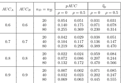
We perform a new simulation to compare pAU C and the proposed bηp,
defined in (2.1), for crossingROC curves only, since in those casesT test doesn’t work properly and pAU C is an alternative to focus on some range of interest. We consider two different ranges (0,0.4) and (0,0.8) although by brevity we only present the results fort0 = 0.4 in Table 7.
Table 7: Power of the partial measures against crossing alternatives. pAU C ηbp AU CA AU CB nD=nD ρ= 0 ρ= 0.5 ρ= 0 ρ= 0.5 20 0.054 0.051 0.031 0.031 0.6 0.6 40 0.140 0.175 0.071 0.078 80 0.255 0.369 0.230 0.314 20 0.042 0.029 0.038 0.051 0.7 0.7 40 0.104 0.117 0.136 0.147 80 0.219 0.296 0.389 0.470 20 0.022 0.024 0.059 0.084 0.8 0.8 40 0.072 0.086 0.207 0.244 80 0.132 0.172 0.470 0.566 20 0.007 0.002 0.071 0.085 0.9 0.9 40 0.032 0.023 0.202 0.247 80 0.069 0.063 0.445 0.555
As can be seen in Table 7,pAU C works better that its counterpartT with higher power in most of the cases. However, our proposed summary statistic ηbp
works much better thanpAU C and similarly to its counterpartbη. That is to say, the new partial summary statistic seems to be a good alternative.
4. REAL DATA EXAMPLES
4.1. Pancreatic cancer biomarker study
The first dataset studied has been used by various statisticians to illustrate statistical techniques for diagnostic tests. First published in [23], it is a case-control study ding 90 cases with pancreatic cancer and 51 case-controls that did not have cancer but who had pancreatitis. Serum samples from each patient were assayed for CA-125, a cancer antigen, and CA-19-9, a carbohydrate antigen, both of which are measured on a continuous positive scale. It can be assumed that both biomarkers are independent. A natural question is to determine which of the two markers best discriminates diseased from healthy subjects. See Figure 2 (a).
FPF
TPF
Empirical ROC curves
FPF TPF 0.0 0.1 0.2 0.3 0.4 0.5 0.6 0.7 0.8 0.9 1.0 0.0 0.2 0.4 0.6 0.8 1.0 CA−19−9 CA−125 FPF TPF
Empirical ROC curves
FPF TPF 0.0 0.1 0.2 0.3 0.4 0.5 0.6 0.7 0.8 0.9 1.0 0.0 0.2 0.4 0.6 0.8 1.0 CA−19−9 CA−125
Figure 2: (a) Empirical ROC curves and (b) Empirical ROC curves once we have eliminated from the data those cases with the smallest values for the second biomarker.
TheAU C[ values are 0.861 and 0.706 for CA-125 (called biomarkerA) and CA-19-9 (called biomarkerB), respectively. TheT statistic, which is based on the methodology described in [6] for paired data, is statistically significantly different from 0 (p = 0.007). The two differences ∆bη =ηbA−bηB and ∆AD =ADA− ADB are also statistically significantly different from 0 (p= 0 and p= 0.015,
respectively). As [23], we have also focus our comparison on the range ofF P F s
The difference is highly significant from 0 based on the bootstrap distribution (p= 0.002 andp= 0, respectively).
In order to illustrate the behaviour of the tests in a different scenario (cross-ingROC curves), we have eliminated from the data those cases with the smallest values for the second biomarker. Therefore, now we consider 80 cases and 51 con-trols. In this case, the two test statistics ∆bη =ηbA−ηbBand△AD =ADA−ADB
are also statistically significantly different from 0 (p = 0) but the statisticT leads us to conclude that both biomarkers are not significantly different (p= 0.128). See Figure 2 (b).
4.2. A method for early recognition of malignant melanoma
The second data set we have considered can be found in [21]. The dataset consists of the clinical scoring scheme without a dermoscope and a dermoscope scoring scheme on 72 suspicious lesions in order to determine whether the der-moscope contributes diagnostic information. The p-value for T for paired data, constructed following [6], is p= 0.882. The p-values for ∆ηband ∆AD are 0.717 and 0.555, respectively. We have also compared both biomarkers through the differences of the partial measures pAU C(0.2) and ηbp(0.2) obtaining p= 0.716
and p= 0.763, respectively. Then, we can conclude that both biomarkers are statistically significantly equal. Therefore, the dermoscope contributes no useful information in this sense.
5. DISCUSSION
There is an interesting relationship between some summary measures for ROC curves and two sample test statistics. Some of them, the Mann-Whitney U-statistic and the Kolmogorov-Smirnov statistic, can be written in terms of functionals of the empirical ROC curve. The former is the well-known AU C
(area under the ROC curve) and the later Youden index. Other test statistics such as Anderson-Darling, Neyman and Watson tests were studied in [16] to assess diagnostic markers. However, it can not be written in terms of functionals of the empiricalROC curve and they do not have value themselves. In this paper, we propose the sum of squared errors between the derivative of the ROC curve and 1, that is the derivative of the 45o line, as aROC summary statistic. This
statistic is closely related to a nonparametric test for two sample problem based on an order statistic introduced in [1]. The exact distribution of this index is known but the simulated version is used ought to computational time since it is checked that the exact test should be essentially the same. For the purpose of
assesing part of a ROC curve, we also define a new partial summary statistic based on the same idea as above but ending the summation as close as possible to the specificF P F of interest.
The simulations show that our ROC summary statistics exhibit much higher power in discriminating between the diseased and healthy distributions and are thus an attractive alternative to ROC-based methodology and indeed constitute in many cases an improvement over AU C and pAU C, respectively. Nevertheless, the fact that our ROC summary statistic does not have value itself is a drawback. The same index value can be obtained for two absolutely different curves. Therefore, after concluding that a new marker is diagnostic, we should study in which way the diseased and healthy distributions are different.
In case of the comparison of two diagnostic markers in the whole range, the use of the difference of our individual ROC summary statistics associated with the two diagnostic markers has higher power than the conventional non-parametric test in [6], the test based on AD test statistic and the permutation test proposed in [21] for crossingROC curves. However, if the primary interest is to detect differences inAU Cs, then the permutation tests of [2] and [4] should be used. On the other hand, when we are interested on a specific range of specificity,
pAU C uses to be an alternative toAU C but we show that our partial summary
statistic ηbp is better to discriminate between two ROC curves that cross each
other when the biomarkers are not correlated as well as when they are correlated.
ACKNOWLEDGMENTS
The authors gratefully acknowledge the constructive comments and sug-gestions of the Associate Editor as well as of an anonymous referee, which led to great improvements in the manuscript. The first author acknowledges support from the project MTM2013-40788-R and the second author from the project MTM2014-55966-P of the Spanish Ministry of Economy and Competitiveness.
REFERENCES
[1] Bairamov, I.G. and Ozkaya, N.¨ (2000). On the nonparametric test for two sample problem based on spacings,J. Appl. Stat. Sci.,10, 57–68.
[2] Bandos, A.I.; Howard, E.R. andGur, D. (2005). A permutation test sensi-tive to differences in areas for comparing ROC curves from a paired design,Stat. Med.,24, 2873–2893.
[3] Bloch, D.A. (1997). Comparing two diagnostic tests against the same “gold standard” in the same sample,Biometrics,53, 73–85.
[4] Braun, T.M. and Alonzo, T.A. (2008). A modified sign test for comparing paired ROC curves,Biostat.,9, 364–372.
[5] Campbell, G.(1994). Advances in statistical methodology for the evaluation of diagnostic and laboratory tests,Stat. Med., 13, 499–508.
[6] DeLong, E.R.; DeLong, D.M. and Clarke-Pearson, D.L. (1988). Comparing the areas under two or more correlated receiver operating charac-teristics curves: A nonparametric approach,Biometrics,44, 837–845.
[7] Gail, M.H. and Green, S.B. (1976). A generalization of the one-sided two-sample Kolmogorov–Smirnov statistic for evaluating diagnostic tests,Biometrics, 32, 561–570.
[8] Greenhouse, S.W.andMantel, N.(1950). The evaluation of diagnostic tests,
Biometrics,6, 399–412.
[9] Hanley, J.A. and McNeil, B.J. (1982). The meaning and use of the area under a receiver operating characteristic (ROC) curve,Radiology,143, 29–36. [10] Hanley, J.A. and McNeil, B.J. (1983). A method of comparing the areas
under receiver operating characteristic curves derived from the same cases, Radi-ology, 148, 839–843.
[11] Linnet, K.(1987). Comparison of quantitative diagnostic tests: Type 1 error, power, and sample size,Stat. Med.,6, 147–158.
[12] Mart´ınez-Camblor, P.; Carleos, C. and Corral, N. (2011). Powerful nonparametric statistics to compare k-independent ROC curves, J. Appl. Stat., 38, 1317–1332.
[13] Mart´ınez-Camblor, P.; Carleos, C.andCorral, N.(2013). General non-parametric ROC curves comparison,J. Korean Stat. Soc.,42, 71–81.
[14] McClish, D.K. (1989). Analyzing a portion of the ROC curve,Med. Decision Making,9, 190–195.
[15] McClish, D.K. (1990). Determining a range of false positive rates for which ROC curves differ,Med. Decision Making,10, 283–287.
[16] Nakas, C.; Yiannoutsos, C.T.; Bosch, R.J. and Moyssiadis, C. (2003). Assessment of diagnostic markers by goodness-of-fit tests,Stat. Med.,10, 2503– 2513.
[17] Obuchowski, N.A.andMcClish, D.K.(1997). Sample size determination for diagnostic accuracy studies involving binormal ROC curve indices, Stat. Med., 16, 1529–1542.
[18] Qin, G.; Jin, X. and Zhou, X.H.(2011). Non-parametric interval estimation for the partial area under the ROC curve,Can. J. of Stat.,39, 17–33.
[19] Shapiro, D.E.(1999). The interpretation of diagnostic tests,Stat. Methods Med. Res.,8, 113–134.
[20] Thompson, M.L.andZucchini, W.(1989). On the statistical analysis of ROC curves,Stat. Med.,8, 1277–1290.
[21] Venkatraman, E.S. and Begg, C.B. (1996). A distribution-free procedure for comparing receiver operating characteristic curves from a paired experiment,
[22] Venkatraman, E.S. (2000). A Permutation Test to Compare Receiver Oper-ating Characteristic Curves,Biometrics,56, 1134–1138.
[23] Wieand, S.; Gail, M.H.; James, B.R. and James, K.L. (1989). A family of nonparametric statistics for comparing diagnostic markers with paired and unpaired data,Biometrika,76, 585–592.
[24] Zhang, D.D.; Zhou, X.H.; Freeman, D.H. and Freeman, J.L. (2002). A non-parametric method for the comparison of partial areas under ROC curves and its application to large health care data sets,Stat. Med.,21, 701–715.
![Table 1 compares the power of b η obtained when the exact distribution studied in [1] is used to obtain the critical values and when 1,000 Monte Carlo replicates are used instead](https://thumb-us.123doks.com/thumbv2/123dok_us/9960029.2488469/8.892.149.723.695.815/table-compares-obtained-distribution-studied-critical-replicates-instead.webp)