Procedia Computer Science 92 ( 2016 ) 188 – 198
1877-0509 © 2016 The Authors. Published by Elsevier B.V. This is an open access article under the CC BY-NC-ND license (http://creativecommons.org/licenses/by-nc-nd/4.0/).
Peer-review under responsibility of the Organizing Committee of ICCC 2016 doi: 10.1016/j.procs.2016.07.345
ScienceDirect
2nd International Conference on Intelligent Computing, Communication & Convergence
(ICCC-2016)
Srikanta Patnaik, Editor in Chief
Conference Organized by Interscience Institute of Management and Technology
Bhubaneswar, Odisha, India
Feature analysis, evaluation and comparisons of classification algorithms based on noisy intrusion
dataset
Jamal Hussain
a, Samuel Lalmuanawma
a* aDepartment of Mathematics & Computer Science, Mizoram University, Aizawl, India, 796004
Abstract
Various studies have been carried on an Intrusion Detection System (IDS) environment bycomparingthe performance of various Machine Learning (ML)based on a refined intrusion dataset with an error-free environment. However, the real-world network data deals with a large amount of noisy information on transmission, and the IDS have to work in such an environment frequently. Dealing with such noisy data is, therefore, a challenging issue in an IDS environment for detecting threads from network activities. In this paper, various Data Mining (DM) and ML algorithms are evaluated and compared by normal and noisy dataset prepared from KDD'99 and NSL-KDD dataset (10%-20% Noise). The empirical results demonstrate that NN (SOM) is far better compared to other tested algorithms regarding robustness tonoisy environment; however,JRip and J48 from the tree family outperform others regarding overall performance matrices. Feature dependency on datasets for a specific classifier is analyzedby Performance-based Method of Ranking (PMR). The evaluation results statistically proved that each classifier has a unique combination of a feature subset to results optimal performance. Empirical results demonstrate that evaluations of IDS based on NSL-KDD give more realistic results compared to theKDD'99 original dataset.
© 2014 The Authors. Published by Elsevier B.V.
Selection and peer-review under responsibility of scientific committee of Missouri University of Science and Technology.
a*
Corresponding Author.Tel:+919436353048 E-mail address: [email protected]
© 2016 The Authors. Published by Elsevier B.V. This is an open access article under the CC BY-NC-ND license (http://creativecommons.org/licenses/by-nc-nd/4.0/).
Keywords:Intrusion Detection System, Machine Learning, anomaly detection, false alarm, ignored attack;
1. Introduction
The advancement of Information Technology (IT) raised numerous security breaches. Therefore, to secure valuable resources over the public network, it is essential to implement an Intrusion Detection System (IDS). IDS aimed to sort out various intrusive attempts on the computer network system based on the three important pillars of information security, i.e., confidentiality, integrity and availability of a resources1. It first gathers and analyze information from various sources within the computer network, triggers alarm to system administrators and blocks unauthorized access if an attack attempt is encountered.
Various recent studies in IDS are evaluated based ona refined intrusion dataset with an error-free environment. However, the real network information deals with a huge amount of noisy data, and the IDS have to work in such an environment repeatedly. Therefore, this paperinvestigates and evaluates on various data mining algorithms to study the performance of each classifier against various datasets,i.e., noise-free and noisy (10% & 20%) environment. We choose top-six classifier from various tested ML algorithms based on evaluating performance. Ranking of significance feature based on performance is done for each selected classifier to study and compare with various feature selection method used in recent research.
2. Theory and Algorithms
2.1.Dataset organization: In this studies, four types of datasets prepared from KDD'99 2and NSL-KDD3intrusion dataset are used to evaluate each classification algorithms. Details of the data preprocess are as follows:
2.1.1. KDD’99 Cup Dataset
This dataset is built and prepared by Stolfoet al.4based on the data captured in DARPA’98 Intrusion Detection
System Evaluation program5.The datasets contain a TCP-dump raw data of about 5 million connections collected from 7 weeks of network traffic records of training sets and 2 weeks records of test set data having around 2 million network traffic records. For each TCP/IP connection, 41 quantitative and qualitative features were extracted. For evaluation, the author used 10% of the original data. After folding the data onto 13 stratified folds, the first folds containing 39461 instances were used for final evaluation.
2.1.2. NSL-KDD Dataset
Tavallaeeetal.3proposed the NSL-KDD datasets thatarean enhanced edition of KDD’99 datasets. The KDD’99
dataset contains large records of redundant data, where 78% training dataset and 75% test dataset are duplicate which may direct classifier algorithm unreasonable towards the further repeated records. Redundant data found on the test dataset can also harm the evaluation performance into a higher degree of detection accuracy. The refined dataset in KDDtrain+.txt and KDDtest+.txt are combined, all the attack traffic in a dataset is grouped into one class named as an anomaly. The ratio of normal and anomaly instances is maintained to meet the preprocess requirement. After folding the data onto six (6) stratified folds, the first fold containing 27526 instances is used for evaluation.
2.1.3. Noisy Dataset (10% & 20%)
Since this studies focus on evaluating the robustness of various data mining algorithms in anoisy environment, the author used the NSL-KDD dataset for noise generation and added noisy data varying percentages of 10% and 20% to specific attributes using the KDD features. Noiseis added to the specific features after analyzing the dependency on thefeature using NSL-KDD. To evaluate and analyzed feature significance, GainRatio6and Info Gain7, based on
k-folds cross-validation technique is used. The author assumed that the noise is added randomly to a specific attributes label and are distributed evenly among the datasets. Every feature can have a noise characteristic, and a few can be cleaned or filtered. However, filtering may require more time complexity and cause delay undesirable for IDS. Besides, for some features, it is not safe to filter away the noise content. Therefore, while performing model evaluation, performance evaluation in the presence of noisy data becomes relevant for the IDS domain.
2.2. Algorithms
The authors utilized the following set of various ML algorithms to study and analyze the applicability and efficiency of a classification algorithm for IDS. The following ML algorithms from various classifier families are evaluated and compared.
Naïve Bayes (NB): NB classifier is based on probabilistic method. It typically relies on assumption and assumes that variables are independent of each class or feature. More specifically, the presence of each particular class or feature is isolated from the absence or occurrence of some other features8. The author9demonstrates its robustness to a noisy environment.
Support Vector Machine (SVM): The basic idea of SVM is to raise dimensions of the samples so that they can be in a separable form. The basic plan is to find a hyperplane to place samples of the same class inside it10.
Artificial Neural Network (NN): An artificial neural network (ANN) is adaptive parallel distributed information processing models. It consists of a set of simple processing units called neurons, a set of synapses, the network architecture and a learning process used to train the network10.
J48: It utilizes a divide-and-conquer approach and recursively create a decision tree based on the greedy algorithm11. It consists of the root node, branches, parent nodes, child nodes and leaf nodes. A node in a tree denotes dataset attributes; every child node derives labeled branches about the possibilities of attribute values from the corresponding node called parent node12.
Bayesian Network (BN): BN is a probabilistic method; representing random variable sets with their conditional dependencies using directed acyclic graph13.
Sequential Minimal Optimization (SMO): SMO is a support vector machines that utilize optimize training method14. Authors used inbuilt libraries in Weka for SMO. It is more sensitive to noise compared to other algorithm9.
Stochastic Variant of Primal Estimated sub-Gradient Solver in SVM (SPegasos): Spegasos used and implements the stochastic variation on the Pegasos technique of Shalev-Shwartzetal.15. All missing values are replaced and transform nominal attributes into binary. All attributes are normalized with the output coefficients are based on the normalized values.
Voted Perceptron (VP): It uses the perceptron algorithm to maps input against one of several feasible non-binary outputs16. The advantages of linearly separable data onto large margins are utilized and are considered to be robust to noisy data 17.
Radial Basis Function Classifier (RBFC): RBF classifier is types of feed-forward network. A general approach is to train the hidden layer of the network based on simple k-means clustering algorithm and the output layer based on supervised learning. However, studies18found that supervised training technique on hidden layer parameters can elevate the performance of prediction. They investigated local variances of the basis functions, learning center locations and attribute weights in a supervised manner.
Ensembles of Balanced Nested Dichotomies for Multi-class Problems (END): END is Meta classifier for managing multi-class data, having 2-class classification strategy by building an ensemble of nested dichotomies. More details of this can be obtained from19.
Stochastic Gradient Descent (SGD): It uses gradient descent optimization technique by taking comparative steps to find local minimum function of the negative gradient based on the objective function, written as a sum of differentiable functions20.
JRip: It is based on the Repeated Incremental Pruning to Produce Error Reduction method. It integrates association rules with reduction error pruning. It divides the dataset into growing sets and pruning set, generating
rules for a subset of the training samples and removes all samples covered by that rules for the training set on all samples21.
Random Forest (RF): RF uses an ensemble technique of unpruned classification; succeed from training data onto the bootstrap samples, using random feature selection in the tree induction process. Final prediction is made based on aggregating the predictions output of the ensemble by majority voting for classification 22.
Decision Table (DT): It is one of the simplest possible hypothesis spaces and is simple enough to be understood. It consists of a hierarchical table where each entry to a higher level table gets broken down into more sub-tables based on the values of a pair of additional attributes forming another table23.
NB-Tree: NB-Tree is proposed by24that integrate a hybrid of decision-tree classifiers and Naïve Bayes classification algorithm. It attempts to utilize the advantages of both decision trees and Naive-Bayes regarding segmentation and evidence accumulation from multiple attributes. A decision tree is built based on univariate splits at every node and Naive-Bayes classifiers at each leaf.
Gaussian Radial Basis Function Network (RBFN): RBF Network uses the simple k-means clustering method to give the basis functions and at the top it uses either a logistic regression or linear regression technique. From each cluster, Symmetric Multivariate Gaussians are fit to the data. It tends to use the given number of clusters per class if the class is nominal. All numeric attributes are standardized to zero mean and unit variance25.
3. Performance analysis
Experimental setup:Experimental environment is carried on Java environment using Weka 3.7.1126 which provides inbuilt libraries containing various machines learning algorithm. The embedded data mining algorithm with default settingsis usedsince most of the relevant studies in Weka used them too. The dataset mentioned in previous sections is preprocessed to meet the ARFF format supported by Weka. Selected 16 classifiers from various classifier families were tested based on k-folds cross-validation (K-FCV) technique within each dataset. K-FCV is one of the most common methods where dataset gets divided into k, k represents the number of folds or subsets, k-1 subsets is used as training sets and k-(k-1) subset is used for thetesting set. More specifically, each fold were analyzed, and the total score results determine the average performance out of k-folds.Our study aimed at two main objectives. Firstly, various classification algorithms were evaluated based on the four datasets to analyze the performance of each model statistically to find the robustness of the analyzed algorithm. Each algorithm was evaluated based on KDD'99, NSL-KDD, 10% Noisy data and 20% Noisy data. A selection of top six classification algorithms is done based on the performance evaluation matrices. Secondly, dependency on each feature based on each classification algorithm was studied using Performance-based Method of Ranking (PMR). Each selected feature subset was once more evaluated on each six classification algorithm to study the effectiveness of each feature selection within each classification algorithms.
Performance evaluation matrices for each simulation result were carefully monitored and measured based on accuracy rate (AC), true positive rate (TPR), false positive rate (FPR), precision, ROC area, # of incorrectly classified rate. RMS error and time complexity is also the key point to measure and determine the reliability of an IDS. Accuracy is the intensity of confidence in detecting intrusive activity. TPR is proportions of instances classified as a given class divided by the actual total in that class (equivalent to Recall). False positive are those normal activities in which the system used to identify as an intrusive attempt. Precision indicates the hit rate of the classification method of detecting intrusive activity. Root Mean Square Error (RMSE) is the distinction between predicting and resultant observed values are each squared and then averaged over the sample. The accuracy of a classification algorithm is measured by Receiver Operating Characteristic (ROC or area under ROC curve), an area of 1 represents a 100% perfect test. Incorrectly classified rate is the rate of false alarm + false negative from the maximum instances, and time complexity is building time in seconds taken to build the model by each classifier.
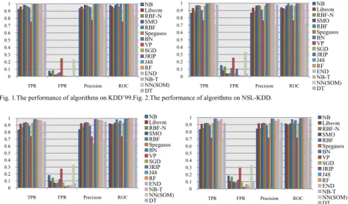
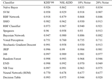
Result analysis: Table 1 and figure 1-4 demonstrate the overall performance of various classification algorithms with each dataset regarding important parameters, i.e., TPR, FPR, Precision and ROC area based on four types of datasets. The evaluation results demonstrate that SGD, Jrip, J48, RF, END and NB-tree results 0.99
Network (SOM) results in the lowest accuracy of 0.77, 0.678, 0.677 and 0.677 based on corresponding datasets (Table 1). Evaluation results derived from NSL-KDD, 10% & 20% noisy datasets results in lower TPR and higher FPR for each evaluated classification algorithms, which was caused by theremoval of redundant instances on NSL-KDD datasets and the existence of noisy information.
Anomaly based IDS suffered from the problem of tension between false alarm and ignored attacks. Reductions of false alarm usually resulted in extra ignored attack rates. So, balance ratios between false alarm rate and ignored attack rate is an important parameter to determine high-quality IDS. False alarm rate is the amount of false positive generated for the abnormal activity. Fig. 5.demonstrate false alarm rate of each evaluated classification algorithms based on each corresponding datasets. DT displays the lowest false alarm rate of 0.16% derived from
KDD’99 dataset while VP results in an extremely high false alarm rate of 38.31% based on theKDD’99dataset.
Fig. 1.The performanceof algorithms on KDD’99.Fig. 2.The performance of algorithms on NSL-KDD.
Figure 3.The performance of algorithms on 10% Noise.Figure 4.The performance of algorithms on 20% Noise.
Ignored attack or alarms are false positives for the normal activity. They are anomaly activity thatis classified as normal cases. Fig 6demonstrate ignored attack rate of each evaluated classification algorithms. RF, NBTree, END, JRip, J48, SMO, RBF and Spegasos results relatively low ignored attack rate based on NSL-KDD dataset. However, NN (SOM) yields relatively high ignored attack rate using NSL-KDD dataset. Overall, JRip and J48 results in more balanced output compared to the others having unbalanced results between each corresponding datasets.
Another important parameter is the time complexity of classification algorithms, RMS error rate and a number of incorrectly classified instances. Time complexity is the time taken by each classification algorithm to build a model within a given set of data and is measured in second (s). # of incorrectly classified instances is the rate of false alarm (Normal instances classified as an anomaly) + False negative (Anomaly instances classified as normal) from the total instances.
Fig. 7.demonstrate the time complexity of each classifier based on various datasets. NB yields the lowest with only 0.19 s derived from both 10% & 20% noisy dataset and proved its robustness to a noisy environment in terms of time complexity. NN (SOM) results in only 0.53 s, 0.59 s, 0.7 s and 1.33 on 20% Noisy, NSL-KDD, 10% noisy
and KDD’99. However, SMO yields relatively high time complexity rate, and authors observed that the addition of noise badly degrades the SMO classification algorithm. Fig. 8 shows that the addition of noisy data in selected features seriously degrades various classification algorithms such as NB, SVM, RBF network, SMO, RBF,
0 0.1 0.2 0.3 0.4 0.5 0.6 0.7 0.8 0.9 1 TPR FPR Precision ROC NB Libsvm RBF-N SMO RBF Spegasos BN VP SGD JRIP J48 RF END NB-T NN(SOM) DT 0 0.1 0.2 0.3 0.4 0.5 0.6 0.7 0.8 0.9 1 TPR FPR Precision ROC NB Libsvm RBF-N SMO RBF Spegasos BN VP SGD JRIP J48 RF END NB-T NN(SOM) DT 0 0.1 0.2 0.3 0.4 0.5 0.6 0.7 0.8 0.9 1 TPR FPR Precision ROC NB Libsvm RBF-N SMO RBF Spegasos BN VP SGD JRIP J48 RF END NB-T NN(SOM) DT 0 0.1 0.2 0.3 0.4 0.5 0.6 0.7 0.8 0.9 1 TPR FPR Precision ROC NB Libsvm RBF-N SMO RBF Spegasos BN VP SGD JRIP J48 RF END NB-T NN(SOM) DT
Spegasos, BN, VP, SGD and DT. However, NN (SOM), JRip, J48, RF, END and NBTree does not change much of their performance and are found to be more robust to the noise environment compared to others.
Figure 5.False alarm rate of classification algorithms.Figure 6. Ignored attack rates of classification algorithms. Table 1.The detection rate of aClassification algorithm for four datasets.
After analyzing each classification algorithm performance based on four datasets, top six classification algorithms are selected based on the weighted evaluation matrices and robustness tonoisy data. Table 2. Shows detail selected classifier that is more robust to the noisy environment. NN (SOM), JRip and J48 are being selected based on its robustness to a noisy environment, while RF, END and NBTree are selected for the overall performance based on the evaluation matrices. However, NN (SOM) yields the lowest accuracy based on each dataset but scores the highest rank based on robustness to anoisy environment. As this study aimed to select a classifier based on the noise tolerance ability, NN (SOM) is, therefore, placed at the first, where JRip J48, NBTree follows. On the other hand, RF and END are selected based on overall performance though they yield relatively high differences between each dataset. 0.00 5.00 10.00 15.00 20.00 25.00 30.00 35.00 40.00 45.00 NB Li bsvm RBF -N SMO RBF Sp eg as o s BN VP SGD JRIP J48 RF EN D NB-T NN(S O M ) DT KDD99 NSL-KDD 10% Noise 20% Noise 0.00 5.00 10.00 15.00 20.00 25.00 30.00 35.00 40.00 NB Li bsvm RBF -N SMO RBF Sp eg as o s BN VP SGD JRIP J48 RF END NB-T NN(S O M ) DT KDD99 NSL-KDD 10% Noise 20% Noise
Classifier KDD’99 NSL-KDD 10% Noise 20% Noise
Naïve Bayes 0.926 0.862 0.833 0.834 SVM 0.958 0.929 0.918 0.907 RBF Network 0.918 0.879 0.868 0.846 SMO 0.982 0.962 0.930 0.913 RBF Classifier 0.973 0.967 0.940 0.921 Spegasos 0.96 0.958 0.93 0.913 Bayesian Network 0.947 0.900 0.886 0.882 Voted Perceptron 0.751 0.760 0.735 0.711
Stochastic Gradient Descent 0.991 0.958 0.930 0.913
JRIP 0.996 0.99 0.984 0.981
J48 0.997 0.989 0.981 0.977
Random Forest 0.998 0.993 0.968 0.946
END 0.998 0.992 0.970 0.949
NB Tree 0.997 0.991 0.963 0.975
Neural Network (SOM) 0.770 0.678 0.677 0.677
Figure 7. Time taken to build model (s). Figure 8.Incorrectly classified and RMS error.
Table 2.Evaluation performance based on robustness to noise.
3.1. Analysis of feature dependency
The dependency of each feature is analyzed based on performance method by ranking each features using selected classification algorithms. This was accomplished by removing unnecessary attributes out of its original dataset. Removal of significant or important features might reduce the performance of the ML algorithm regarding detection accuracy. However, removal of some features that might have ahigh degree of noise or might not have contributions in any way can extensively advance the performance and search speed of a classification algorithm (Lin et al., 2008).
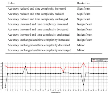
For PMR, one feature is removed from the dataset at a time, the resultant features subset data is then used for training and testing each selected classifier (based on k-folds cross-validation method). Then the evaluation performance of the analyzed classifier is compared with the original classifier derived from the original attributes (41 features overall accuracy). Final ranking (significant, insignificant and minor) of a feature is done using the decision rules set (Table 3) based on the overall accuracy and time complexity. The algorithm below is used to select performance based ranking method.
Algorithm 1: Performance-based method ranking
1. Choose one classification algorithm
2. Read supplied original dataset (with 41 features set)
3. Train and test the classifier (original set)
4. Dothe following procedure foreach feature
a) Removeone feature out of 41 from the dataset (one at a time)
b) Use the resultant subset data to trainand testthe classifier
c) Compare performance results of the classifier with the original
d) Based on the decision rules set(Table 3) rank the analyzed feature
e) Continuetill all feature are analyzed
5. End 0 1000 2000 3000 4000 5000 6000 7000 8000 KDD99 NSL-KDD 10% Noise 20% Noise Ti m e ( S ) Data sets NB Libsvm RBF-N SMO RBF Spegasos BN VP SGD JRIP J48 RF END NB-T NN(SOM) DT 0.00 5.00 10.00 15.00 20.00 25.00 30.00 35.00 # of in correct ly cl assi fi ed RM S e rro r # of in correct ly cl assi fi ed RM S e rro r # of in correct ly cl assi fi ed RM S e rro r # of in correct ly cl assi fi ed RM S e rro r KDD99 NSL-KDD 10% Noise 20% Noise Data sets NB Libsvm RBF-N SMO RBF Spegasos BN VP SGD JRIP J48 RF END NB-T NN(SOM) DT
Classifier NSL-KDD 10% Noise Differences % 20% Noise Differences %
NN (SOM) 0.678 0.677 0.15 0.677 0.15 JRip 0.99 0.984 0.61 0.981 0.91 J48 0.989 0.981 0.81 0.977 1.21 NBTree 0.991 0.963 2.83 0.975 1.61 END+ND+RF 0.992 0.97 2.22 0.949 4.33 RF 0.993 0.968 2.52 0.946 4.73
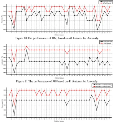
Based on the above algorithm, each 41 features are ranked using decision rules set (table 3) for each selected top 6 classification algorithms. Out of 41 original features, a 16 features subset <2, 3, 4, 23, 24, 27, 28, 29, 30, 31, 35, 36, 37, 38, 39, 40> are significant features selected by NN (SOM) fig. 10, 37 features subset <1, 2, 3, 4, 5, 8, 9, 10, 11, 12, 13, 14, 15, 16, 17, 18, 19, 20, 21, 22, 23, 24, 27, 28, 29, 30, 31, 32, 33, 34, 35, 36, 37, 38, 39, 40, 41> by JRip fig. 11, 23 features subset <2, 3, 4, 6, 10, 12, 14, 16, 17, 22, 24, 25, 26, 28, 32, 34, 35, 36, 37, 38, 39, 40, 41> by J48 fig. 12, 35 features subset <1, 2, 3, 4, 5, 6, 7, 8, 9, 10, 11, 12, 13, 14, 15, 16, 17, 22, 23, 24, 25, 26, 27, 28, 29, 32, 33, 34, 35, 36, 37, 38, 39, 40, 41> by RF fig. 13, 28 features subset <1, 3, 4, 7, 8, 10, 12, 14, 15, 17, 19, 20, 21, 22, 23, 24, 25, 26, 28, 29, 30, 32, 35, 36, 37, 39, 40, 41> by END fig. 14 and 33 features subset <1, 2, 3, 7, 8, 9, 10, 11, 12, 13, 14, 15, 16, 17, 18, 20, 21, 22, 23, 24, 25, 26, 28, 30, 32, 34, 35, 36, 37, 38, 39, 40, 41> are selected based on NBTree fig. 15. Comparisons of each classification algorithm based on Time complexity are shown in fig. 16.
Table 3. Decision rules set based on performance.
Rules Ranked as
Accuracy reduced and time complexity increased Significant
Accuracy reduced and time complexity reduced Significant
Accuracy reduced and time complexity unchanged Significant
Accuracy increased and time complexity increased Insignificant
Accuracy increased and time complexity decreased Insignificant
Accuracy increased and time complexity unchanged Insignificant
Accuracy unchanged and time complexity increased Insignificant
Accuracy unchanged and time complexity decreased Minor
Accuracy unchanged and time complexity unchanged Minor
1 2 3 4 5 6 7 8 91011121314151617181920212223242526272829303132333435363738394041 54 56 58 60 62 64 66 68 70 Accuracy (%) Deleted feature NN-SOM(Anomaly) NN-SOM(W.avg)
Figure 9.The performance of Neural Network (SOM) based on 41 features for Anomaly.
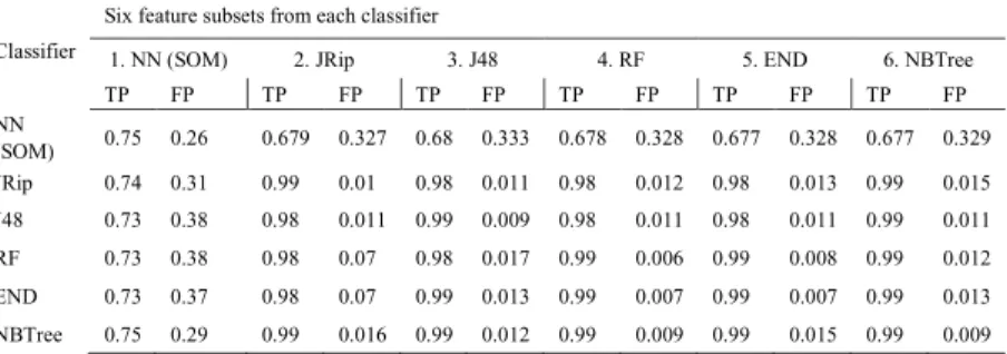
To evaluate the reliability of the performance-based method ranking feature selection, the six feature subsets selected by each classifier are again evaluated and tested for each six classification algorithm (Table 4). Here, each feature subsets are evaluated using six classifiers until all six feature subsets are tested and analyzed. It is being observed that each performance based feature ranking method of each classification algorithm has a unique subset of features. Each feature subset selected by individual classifier is the best for the based classification algorithm. Therefore, it is seen that, feature subset selected by NN (SOM) classifier resulting 0.75 TP, 0.74 TP, 0.73 TP, 0.73 TP, 0.73 TP, 0.75 TP for NN (SOM), JRip, J48, RF, END and NBTree where 0.75 TP with only 0.26 FP based on NN (SOM) classifier is selected as an optimal performance for the analyzed feature subset.JRip classifier shows 0.679 TP, 0.99 TP, 0.98 TP, 0.98 TP, 0.98 TP, 0.99 TP for NN(SOM), JRip, J48, RF, END and NBTree respectively, showing that 0.99 TP with only 0.01 FP is scored based on the JRip classifier for the analyzed feature subset. The same observations for each classification algorithms J48, RF, END and NBTreeis shown in Table 4.
1 2 3 4 5 6 7 8 91011121314151617181920212223242526272829303132333435363738394041 98.5 98.6 98.7 98.8 98.9 99.0 Accuracy (%) Deleted feature JRip(Anomaly) JRip(W.avg)
Figure 10.The performance of JRip based on 41 features for Anomaly.
1 2 3 4 5 6 7 8 91011121314151617181920212223242526272829303132333435363738394041 98.3 98.4 98.5 98.6 98.7 98.8 98.9 99.0 Accuracy (%) Deleted feature J48(Anomaly) J48(W.avg)
Figure 11.The performance of J48 based on 41 features for Anomaly.
1 2 3 4 5 6 7 8 91011121314151617181920212223242526272829303132333435363738394041 98.9 99.0 99.1 99.2 99.3 99.4 Accuracy (%) Deleted feature Random Forest(Anomaly) Random Forest(W.avg)
Figure 12.The performance of Random Forest based on 41 features for Anomaly.
1 2 3 4 5 6 7 8 91011121314151617181920212223242526272829303132333435363738394041 99.00 99.05 99.10 99.15 99.20 99.25 99.30 99.35 99.40 Accuracy (%) Deleted feature END(Anomaly) END(W.avg)
Figure 13.The performance of END based on 41 features for Anomaly.
1 2 3 4 5 6 7 8 91011121314151617181920212223242526272829303132333435363738394041 98.5 98.6 98.7 98.8 98.9 99.0 99.1 Accuracy (%) Deleted feature NBTree(Anomaly) NBTree(W.avg)
Figure 14.The performance of NB Tree based on 41 features for Anomaly. 1 2 3 4 5 6 7 8 910 11 12 13 14 15 16 17 18 19 20 21 22 23 24 25 26 27 28 29 30 31 32 33 34 35 36 37 38 39 40 41 0 20 40 60 80 100 120 140 Time (s) Deleted feature NEURAL NETWORK(SOM) JRIP J48 RANDOM FOREST END NB TREE
Figure 15.The time complexity of each classifier based on 41 features for Anomaly.
Table 4.The performance of each classification algorithms based on six feature subsets.
4. Conclusions
In this paper, the performance of various classification algorithms has been compared and evaluated based on
KDD’99 dataset, NSL-KDD dataset, and a noise-added dataset. Various classification algorithms like NB, SVM, RBF Network, SMO, RBF classifier, Spegasos, BN, VP, SGD, JRIP, J48, RF, END, NB-Tree, NN (SOM), DT from various classification algorithm families were tested and compared.
Finally, the comparison results of show that recent studies from various classification algorithms in the absence of noisy environment or noise free dataset could misinform about evaluation performance to a much higher degree. The empirical results demonstrate that the algorithm thatperforms well on the original KDD’99 dataset does not
result in the same with NSL-KDD, 10% noisy data and 20% noisy data, which proves that the NSL-KDD dataset represents more realistic environment for evaluation of classification algorithms compared to theKDD’99dataset.
Among various tested classification algorithms, JRip and J48 were generally (overall performance, fig. 1-4) advanced compared to the other tested algorithms followed by RF, END and NB-Tree. However, Neural Network (SOM) is far more superior to all the others regarding robustness to a noisy environment (Table 2). The presence of noise in the datasets does not harm the performance of the algorithm (i.e., 10% & 20% noisy data).
The studies of feature selection evaluation based on Performance-based Method of Ranking statistically show thateach classification algorithm has unique combinations of feature subset for the best optimal performance (Table 4). Empirical results statistically demonstrate that the feature subsets selected by each classification algorithm are different from each other; dependency of each feature subset depends on the type of classification algorithm. It is provedthat, each classification algorithm has its unique combination of feature subsets. In other words, the use of significant or dependent features based on PMR for each class in a given classifier results in the most
Classifier
Six feature subsets from each classifier
1. NN (SOM) 2. JRip 3. J48 4. RF 5. END 6. NBTree
TP FP TP FP TP FP TP FP TP FP TP FP NN (SOM) 0.75 0.26 0.679 0.327 0.68 0.333 0.678 0.328 0.677 0.328 0.677 0.329 JRip 0.74 0.31 0.99 0.01 0.98 0.011 0.98 0.012 0.98 0.013 0.99 0.015 J48 0.73 0.38 0.98 0.011 0.99 0.009 0.98 0.011 0.98 0.011 0.99 0.011 RF 0.73 0.38 0.98 0.07 0.98 0.017 0.99 0.006 0.99 0.008 0.99 0.012 END 0.73 0.37 0.98 0.07 0.99 0.013 0.99 0.007 0.99 0.007 0.99 0.013 NBTree 0.75 0.29 0.99 0.016 0.99 0.012 0.99 0.009 0.99 0.015 0.99 0.009
optimalperformance.
The results of our studies and evaluation encourage us to carry on further research on various hybrid IDS techniques. Exploration of various uncovered classification algorithms against real network traffic along with the effect of various feature dependent selection method will be the focus of our future works.
References
1. Bishop M. Introduction to computer security. Addison-Wesley Professional; 2004.
2. KDD Cup 1999: Computer Network Intrusion Detection http://www.sigkdd.org/kdd-cup-1999-computer-network-intrusion-detection
3. Quinlan JR. Introduction of decision trees. Machine Learning1986; 1: 81–106.
4. Tavallaee M, Bagheri E, Lu W, Ghorbani A. A detailed analysis of the KDD CUP 99 data set. In: Proceeding of the IEEE symposium on computational intelligence for security and defense applications;2009. p. 53–58.
5. Stolfo SJ, Fan W, Lee W, Prodromidis A, Chan PK. Cost based modeling for fraud and intrusion detection: Results from the jam project. In: Proceedings of DARPA Information survivability conference and exposition, DISCEX '00; 2000. 2. p 130-144.
6. Lippmann RP, Fried DJ, Graf I, Haines JW, Kendall KR, McClung D, Weber D, Webster SE, Wyschogrod D, Cunningham RK, Zissman MA. Evaluating intrusion detection systems: the 1998 DARPA off-line intrusion detection evaluation.In Proceedings of the DARPA Information survivability conference and expositionDISCEX '00; 2000. p. 12-26.
7. Liu H, Setiono S. Chi2: Feature Selection and Discretization of Numeric Attributes. In: Proceedings of the 7th IEEE International conference on Tools with artificial intelligence (TAI '95); 1995. p. 88-90.
8. Ganchev T, Zervas P, Fakotakis N, Kokkinakis G. Benchmarking feature selection techniques on the speaker verification task.In: Proceeding of the 5th International symposium on Communication system, network and digital signal processing; 2006. p. 314-318.
9. George H. John, Langley P (1995). Estimating Continuous Distributions in Bayesian Classifiers.In Proceedings of the 11th Conference on uncertainty in artificial intelligence, Morgan Kaufmann, San Mateo; 1995. p. 338-345.
10. Nettleton DF, Puig AO, Fornells A. A study of the effect of different types of noise on the precision of supervised learning techniques. Artificial Intelligence Review2010; 33(4): 275-306.
11. Ghorbani AA, Lu W, Tavallaee M. Network Intrusion Detection and Prevention Concepts and Techniques, Springer New York Dordrecht Heidelberg London; 2010.
12. Kim G, Lee S, Kim S. A novel hybrid intrusion detection method integrating anomaly detection with misuse detection.Expert Systems with Applications2014; 41(4): 1690–1700.
13. Pearl J. (1985). Bayesian Networks: A Model of Self-Activated Memory for Evidential Reasoning (UCLA Technical Report CSD-850017). In Proceedings of the 7th Conference of the Cognitive science society, University of California, Irvine, CA; 1985. p. 329–334.
14. Platt JC. Sequential Minimal Optimization: A Fast Algorithm for Training Support Vector Machines. In Proceedings of International conference on Advance in kernel methods - Support vector learning; 1998.
15. Shwarz SS, Singer Y, Srebro N. Pegasos: Piramal estimated sub-gradient solver for SVM. In: Proceedings of the 24th International conference on machine learning; 2007. p. 807-814.
16. Freund Y, Schapire RE. Large margin classification using the perceptron algorithm.Machine Learning1999; 37(3): 277-296.
17. Khardon R, Wachman G. Noise tolerant variants of the perceptron algorithm. The Journal of Machine Learning Research2007; 8: 227-248.
18. Wettschereck D, Dietterich T. Improving the performance of radial basis function networks by learning center locations. In Neural Information Processing Systems 4. Denver, CO: Morgan Kaufmann NIPS 1992; 4: 1133–1140.
19.Dong L, Frank E, Kramer S. Ensembles of balanced nested dichotomies for multiclass problems. In: Proceedings of the 9th European
conference on Principles and practice of knowledge;2005.
20. Bottou L. Online Algorithms and Stochastic Approximations. Online Learning and Neural Networks.Cambridge University Press; 1998.
21. Cohen WW. Fast effective rule induction. In Proceedings of the 12th International Conference on Machine learning; 1995. p. 115–123.
22. Breiman L. Random Forests. Machine Learning2001; 45(1): 5-32.
23. Kohavi R. The power of decision tables.In: Proceedings of the 8th European Conference on Machine Learning; 1995. p. 174-189. 24. Kohavi R. Scaling up the accuracy of Naive Bayes Classifier: a Decision-Tree Hybrid. In: Proceedings of the 2nd International conference
on knowledge discovery and data mining; 1996. p. 202-207.
25. Howlett RJ, Lakhmi CJ. Radial Basis Function Networks 2: New Advances in Design. Springer-Verlang Berlin Heidelberg; 2001.
26. Hall M, Frank E, Holmes G, Pfahringer B, Reutemann P, Witten IH. The WEKA data mining software: An update. ACM SIGKDD Explorations Newsletter2009; 11(1): 10–18.