Image-Based Localization Using Deep Neural Networks

(1)

Image-Based Localization Using Deep

Neural Networks

Xiaotian Li

School of Electrical Engineering

Thesis submitted for examination for the degree of Master of Science in Technology.

Espoo 2.10.2017

Thesis supervisor:

Prof. Juho Kannala

Thesis advisor:

(2)

aalto university

school of electrical engineering

abstract of the master’s thesis

Author: Xiaotian Li

Title: Image-Based Localization Using Deep Neural Networks

Date: 2.10.2017 Language: English Number of pages: 6+72

Degree programme: Automation and Electrical Engineering Major: Control, Robotics and Autonomous Systems

Supervisor: Prof. Juho Kannala Advisor: D.Sc. (Tech.) Juha Ylioinas

Image-based localization, or camera relocalization, is a fundamental problem in computer vision and robotics, and it refers to estimating camera pose from an image. It is a key component of many computer vision applications such as navigating autonomous vehicles and mobile robotics, simultaneous localization and mapping (SLAM), and augmented reality.

Currently, there are plenty of image-based localization methods proposed in the literature. Most state-of-the-art approaches are based on hand-crafted local features, such as SIFT, ORB, or SURF, and efficient 2D-to-3D matching using a 3D model. However, the limitations of the hand-crafted feature detector and descriptor become the bottleneck of these approaches. Recently, some promising deep neural network based localization approaches have been proposed. These approaches directly formulate 6 DoF pose estimation as a regression problem or use neural networks for generating 2D-3D correspondences, and thus no feature extraction or feature matching processes are required.

In this thesis, we first review two state-of-the-art approaches for image-based localization. The first approach is conventional hand-crafted local feature based (Active Search) and the second one is novel deep neural network based (DSAC).

Building on the idea of DSAC, we then examine the use of conventional RANSAC and introduce a novel full-frame Coordinate CNN. We evaluate these methods on the 7-Scenes dataset of Microsoft Research, and extensive comparisons are made. The results show that our modifications to the original DSAC pipeline lead to better performance than the two state-of-the-art approaches.

Keywords: computer vision, machine learning, deep neural networks, image-based localization

(3)

iii

Preface

This thesis was carried out under the supervision of Prof. Juho Kannala, and I would like to thank him for his guidance and support. I am grateful to my advisor Dr. Juha Ylioinas for all the help. Finally, I would like to thank my family for the love and constant encouragement.

Otaniemi, 02.10.2017

(4)

iv

Abbreviations and Acronyms

ANN Artificial Neural Network

CNN Convolutional Neural Network

DLT Direct Linear Transformation

DNN Deep Neural Network

DoF Degrees of Freedom

DSAC Differentiable Sample Consensus

ELU Exponential Linear Unit

FCN Fully Convolutional Network

FLANN Fast Library for Approximate Nearest Neighbors

GPS Global Positioning System

IBL Image-Based Localization

LSTM Long-Short Term Memory

MLP Multilayer Perceptron

ORB Oriented FAST and Rotated BRIEF

PnP Perspective-n-Point

RANSAC Random Sample Consensus

ReLU Rectified Linear Unit

RGB Red-Green-Blue

RGB-D Red-Green-Blue-Depth

SCoRF Scene Coordinate Regression Forests

SfM Structure from Motion

SIFT Scale Invariant Feature Transform

SLAM Simultaneous Localization and Mapping

SURF Speeded Up Robust Features

(7)

1 Introduction

Image-based localization (IBL) is an important problem in computer vision and robotics. It addresses the problem of estimating the 6 DoF camera pose in an environment from an image. Recently, with the widespread use of smartphones equipped with modern cameras, IBL has received increasing attention since it is an important component of many interesting applications such as robot localization [10], simultaneous localization and mapping (SLAM) [13], place recognition [40], and augmented reality [6, 43].

There are also other forms of localization available to smartphones such as GPS and WiFi based localization. Unfortunately, GPS is only suitable for outdoor, rather than indoor environments, and is often inaccurate in urban environments with tall buildings. Although WiFi based localization is a good alternative for indoor environments, it, however, suffers several drawbacks. For example, its accuracy critically depends on the number of available access points, thus requiring the setup and maintenance of a significant number of devices, especially for large buildings. Besides, WiFi based localization system cannot provide the orientation of a user, thus being unsuitable for augmented reality applications.

Unlike GPS or WiFi based localization approaches, image-based localization does not have these limitations. It can be operated in both indoor and outdoor environments using the low-cost camera without the setup and maintenance of infrastructure. In addition, with the rapid development of computer vision, image-based localization is becoming more and more robust and accurate.

1.1 Problem Statement

Currently, there are plenty of image-based localization methods proposed in the literature. Most state-of-the-art approaches [56, 57, 58] are based on local features, such as SIFT, ORB, or SURF [42, 54, 2], and efficient 2D-to-3D matching. Given a 3D scene model, where each 3D point is associated with the image features from which it was triangulated, localizing a new query image against the model is solved by first finding a large set of matches between 2D image features and 3D points in the model via descriptor matching, and then using RANSAC [15] to reject outlier matches and estimate the camera pose on inliers. Although these local feature based methods have been proven to be very accurate and robust in many situations (mainly in outdoor environments), due to the limitations of the hand-crafted feature detector and descriptor, extremely large viewpoint changes, occlusions, repetitive structures and textureless scenes often produce a large number of false matchings which will lead to localization failure. Therefore, indoor image-based localization is still a very challenging problem since indoor scenes often have repetitive structures, less texture and insufficient local features for matching.

Recently, some promising neural network based localization approaches have been proposed. Approaches such as PoseNet [33] formulate 6 DoF pose estimation as a regression problem, and thus no traditional feature extraction, feature description, or feature matching processes are required. It has been shown that these approaches

(8)

2 overcome the limitations of the local feature based approaches, i.e., they are able to recover the camera pose in very challenging indoor environments where the traditional methods fail. However, their localization performance is still far below traditional approaches in other situations where local features perform well. Unlike PoseNet, approaches such as DSAC [3] obtain the 6 DoF pose by a two-stage pipeline: first, regressing a 3D point position for each pixel in an image and, then, determining the camera pose using RANSAC based on these correspondences as in the conventional localization pipeline. Although these methods require depth maps associated with input images at training time, their localization performance even surpasses the state-of-the-art local feature based approaches on indoor scenes.

In this thesis, the main task is to determine how well a state-of-the-art neural network based method can perform compared to a state-of-the-art conventional local feature based method and how can we improve upon the state-of-the-art neural network based method. We first review two state-of-the-art approaches for image-based localization. The first approach is Active Search [57, 58] which is conventional hand-crafted local feature based. The second approach is DSAC [3] based on patch-based Coordinate CNN and novel differentiable RANSAC. We then further explore the DSAC method and examine the use of conventional RANSAC in the DSAC pipeline. Finally, a novel full-frame Coordinate CNN is introduced. Experiments on a widely used dataset are conducted to evaluate the performance of these approaches.

1.2 Structure of the Thesis

The rest of the thesis is structured as follows. In Chapter 2, the background literature related to image-based localization and deep neural networks is presented. Here we give a brief introduction to several IBL methods and the building blocks of the neural network based methods. The detailed descriptions of the two state-of-the-art methods, Active Search and DSAC, are presented in Chapter 3 and 4 respectively. Chapter 5 discusses the modifications to the DSAC method. Chapter 6 describes the details of experiments and presents results of the experiments to determine the performance of the discussed methods and provide extensive comparisons between them. In Chapter 7, we discuss the results, and some directions of future study are given. Finally, Chapter 8 summarizes and concludes this thesis.

(9)

3

2 Background

Before diving deeper, we first review the theoretical background necessary for un-derstanding the approaches discussed in the rest of the thesis. This includes a brief introduction to the history of image-based localization and some approaches to solving the localization task. Additionally, we present the theoretical background on deep neural networks required for the better understanding of the neural network based approaches.

2.1 Image-Based Localization

Solving the image-based localization problem consists of estimating the 6 DoF camera pose (3 DoF position and 3 DoF orientation) of a query image in an arbitrary scene. This is also known as camera relocalization. More specifically, the localization system takes only one image as input, and then outputs camera pose according to a given representation of the scene. The representation of the scene depends on the approach used. It can be a database of images, a reconstructed 3D model, or a trained deep neural network. Here we only consider one image as input, although the image-based localization task can be extended by using a sequence of images as input. The input images are usually RGB-only without depth information, since current low-cost devices are not commonly equipped with depth sensors.

In the earliest stages, image-based localization was solved by treating it as a location recognition problem [75]. In these approaches, image retrieval techniques are often applied to determine the location of the query image by matching it to a database of images and finding the most similar images to it. The locations of the database images are known. Thus, the location of the query image can be estimated according to the known locations. Initially, these methods worked on databases consisting of tens of thousands of images and then they were improved to deal with more than a million images. However, the localization performance provided by these approaches is limited by the accuracy of the known locations of the database images [56] and the density of the key-frames.

To obtain a better localization performance, more recent techniques [29] are based on more detailed and structured information, i.e., they use a reconstructed 3D point cloud model, usually obtained from Structure-from-Motion, to represent the scene. This is enabled by some powerful SfM approaches such as Bundler [63]. It is even possible to construct huge models with millions of points [65]. Thus, image-based localization systems are enabled to work on a city-scale level.

Instead of matching the query image to the database images, these keypoint based methods solve the localization task by finding correspondences between the query image and the 3D model. This is achieved by the use of the conventional hand-crafted features, e.g., SIFT [42]. The features of the 3D points are computed during the 3D reconstruction, and the features of the query image are detected and extracted at test time. Therefore, the correspondence search is formulated as a descriptor matching problem. After establishing the 2D-3D correspondences, the camera pose is determined by a Perspective-n-Point [35] solver inside a RANSAC

(10)

4 [15] loop.

It is obvious that the pose estimation step can only succeed if the quality of the established correspondences is good enough. When the 3D model is too big in size or too complex, an efficient and effective descriptor matching step is essential. There are several techniques in the literature to handle this problem, such as 2D-to-2D-to-3D matching [29], 3D-to-2D-matching [40], prioritized matching [56] and co-visibility filtering [57]. However, even if the matching process is enough effective and efficient, limitations of the hand-crated features will still cause these keypoint based localization systems to fail.

Recently, it has been shown that machine learning methods have great potential to tackle the problem of image-based localization. PoseNet [33] demonstrates the feasibility of formulating 6 DoF pose estimation as a regression problem. The pose of a query image is directly regressed by a deep CNN with GoogLeNet [66] architecture pre-trained on large-scale image classification data. However, its performance is still below the state-of-the-art keypoint based methods and far from ideal for practical camera relocalization. In order to improve the accuracy of PoseNet, several variants have been proposed in recent papers. For example, LSTM-Pose [69] makes use of LSTM units [26] on the CNN output to exploit the structured feature correlation. The LSTM units play the role of a structured dimensionality reduction on the feature vector and lead to drastic improvements in localization performance. Another variant, Hourglass-Pose [48], is based on hourglass architecture which consists of a chain of convolution and upconvolution layers followed by a regression part. The upconvolution layers are introduced to preserve the fine-grained information of the input image and this mechanism has been proven to be able to further improve the accuracy of image-based localization using CNN based architectures. Besides, it has been shown that the use of a novel loss function based on scene reprojection error can also significantly improve PoseNet’s performance [32].

Unlike PoseNet, the scene coordinate regression forests (SCoRF) approach [61] adopts a regression forest [9] to generate 2D-3D matches from an RGB-D input image instead of directly regressing the camera pose. The final camera pose is then determined via a RANSAC based solver. This whole pipeline is similar to the keypoint based localization approaches, but no traditional feature extraction, feature description, or feature matching processes are required. The original SCoRF pipeline is further improved by exploiting uncertainty in the model [68]. Training the random forest to predict multimodal distributions of scene coordinates results in increased pose accuracy. Although these methods are extremely accurate, they require depth information during test time.

In order to localize RGB-only images as well, the original SCoRF is extended by utilizing the increased predictive power of an auto-context random forest [4]. In the most recent DSAC paper [3], a neural network based SCoRF pipeline for RGB-only images is proposed. In contrast to previous SCoRF pipelines, two CNNs are adopted for predicting scene coordinates and for scoring hypotheses. Moreover, the conventional RANSAC is replaced by a new differentiable RANSAC, which enables the whole pipeline to be trained end-to-end.

(11)

5

2.2 Approaches to Localization

In this section, we present three approaches to solve the localization problem related to this thesis.

2.2.1 Keypoint Based Localization

In order to determine the full camera pose, i.e., both position and orientation, we need to know the detailed 3D structure of the scene. Fortunately, such a 3D model of discriminative feature points can be obtained efficiently from a set of images using modern Structure-from-Motion techniques. During the reconstruction process, as each 3D point is obtained by triangulation made on corresponding image features, every 3D point in sparse point cloud model is already associated with feature descriptors. Thus, registering a 2D image to the 3D model can be solved by matching 2D image points and 3D model points. Then, the pose of the query image can be solved by feeding theses 2D-3D correspondences into a PnP [35] algorithm. Since the correspondences are usually not perfect but rather noisy, the PnP algorithm is used in combination with random sample consensus (RANSAC) [15] to be robust to outliers.

Keypoint based localization problem is essentially a descriptor matching problem. However, if the 3D point cloud model is too large or dense, the descriptor matching is typically inaccurate and computationally expensive. Therefore, several matching techniques have been proposed to make the descriptor matching efficient and effective. The matching techniques can be divided into two main classes: indirect and direct matching. Indirect matching approaches usually use an intermediate construct to represent the 3D point descriptors. For example, since 3D point descriptors are generated from database images, we can establish 2D-3D correspondences by first finding database images similar to the query image and then matching the query image against these database images (2D-to-2D-to-3D matching). Another example is to do 3D-to-2D matching, i.e., matching the model against the query image with co-visibility information. Contrary to indirect matching, direct matching techniques directly match the 2D image features against 3D points, i.e., they try to find the nearest neighbors of a 2D image feature in the space containing the 3D point descriptors.

It has been shown that classical direct matching techniques such as approximative tree-based search [49] achieve a better performance than indirect matching techniques, but they are much more computationally expensive, especially when the 3D point cloud model is very large and dense. In contrast, indirect matching methods are memory efficient and extremely faster than direct matching. However, they are not effective as they are more prone to fail to register an image.

In order to perform the matching both efficiently and effectively, Active Search [57, 58], which combines direct matching and indirect matching via a visual vocabulary based prioritization scheme, has been proposed. More details of Active Search are presented in Chapter3.

(12)

6

2.2.2 PoseNet

PoseNet [33] first demonstrates the feasibility of casting pose estimation of a single RGB image as a regression problem and solves it using a deep neural network. Contrary to formulating localization as a classification problem which can estimate only the position of the image, this method recovers the full camera pose p= [x,q], where xis the 3D camera position andqis a quaternion representing the orientation. The PoseNet system is simple. Only a convolutional neural network is used to estimate the camera pose. Therefore, it only takes 5ms to run, meeting the real-time requirement of many applications [33]. However, its localization performance is far below the state-of-the-art methods.

To regress pose, the convolutional neural network is trained in an end-to-end manner with the following objective loss function:

loss(I) =kxˆ−xk2+βkqˆ−

q

kqkk2 (1)

where [x,q] and [ˆx,qˆ] are ground truth pose and estimated pose respectively. Here

β is a coefficient used to balance the position and orientation errors, and thus it is in general bigger for outdoor scenes due to larger positional error [33]. It has been found that learning position and orientation jointly can achieve better results than learning to regress them separately. Since the orientation here is represented by quaternions and the network cannot be regularized to generate only valid unit quaternions, the estimated quaternion should be normalized.

PoseNet adopts GoogLeNet model [66] as a basis to do pose regression. The final PoseNet architecture is illustrated in Figure 1. Some modifications are made to the original GoogLeNet architecture:

– All three softmax classifiers are replaced by affine regressors.

– A fully connected layer of width 2048 is added before the final regressors. In addition, it has been shown that leveraging the idea of transfer learning to start the pose training from a network pre-trained on giant ImageNet [12] and Places [76] datasets can result in better localization performance and allow training on only a few examples.

A number of variants of PoseNet have been proposed to improve the localization performance, such as LSTM-Pose [69] and Hourglass-Pose [48]. Their architectures are illustrated in Figure 2 and Figure3 respectively.

2.2.3 Scene Coordinate Regression Forests

Scene coordinate regression forests (SCoRF) [61] system is similar to the traditional keypoint based approaches: first generates point correspondences and then determines the final pose inside a RANSAC loop. However, unlike the traditional methods which formulate the 2D-3D correspondence search as a descriptor matching problem, SCoRF uses a regression forest [9] to directly regress the 3D scene coordinates in

(13)

7

Figure 1: Architecture of PoseNet. Conv and fc are the convolutional layer and fully connected layer respectively (described in Section2.3.3). Icp is the Inception module of GoogLeNet [66]. Figure adapted from [71].

Figure 2: Architecture of LSTM-Pose. Figure adapted from [69].

the world space from the pixels of an RGB-D query image. Since at test time, the 3D coordinates of image pixels in camera space can be computed from the depth information and known camera intrinsics, 2D-3D correspondences become 3D-3D correspondences and the final pose is solved by the Kabsch algorithm [31] instead of the PnP algorithm. The whole SCoRF pipeline is illustrated in Figure 4.

In the SCoRF pipeline, the dense 2D pixel to 3D scene coordinate correspondences are learned using a dataset of RGB-D images. The ground truth camera poses of these images are obtained using KinectFusion [30, 51]. Using the known camera intrinsics, the depth information and the ground truth camera poses, 3D world coordinates of image pixels can be determined. This gives the ground truth 2D-3D correspondences. Then, a regression forest is trained using these correspondences. Both RGB and depth features at a pixel location are used by this regression forest to predict the corresponding 3D position of the pixel in the world space. Because the forest is trained using the densely sampled 2D-3D correspondences, it can be evaluated at any pixel location of a test image. Therefore, at test time, the forest can be efficiently applied to only a sparsely sampled set of image pixels to generate 2D-3D

(14)

8

Figure 3: Architecture of Hourglass-Pose. Figure adapted from [48].

correspondences. In this way, the regression forest can be seen as an implicit 3D map of the scene. Finally, with this sparse set of correspondences and the computed 3D coordinates in camera space, an adapted version of preemptive RANSAC is used to obtain an accurate final camera pose.

The SCoRF localization pipeline has been extended in several works. In the recent DSAC paper [3], an RGB-only CNN-based SCoRF pipeline is introduced. The DSAC method is explained in detail in Chapter4.

2.3 Artificial Neural Networks

Deep learning is currently one of the most popular and important research topics in machine learning, computer vision and artificial intelligence.

Traditional artificial neural networks (ANNs) are usually composed of one input layer, one output layer, and a few hidden layers in between. Deep neural networks (DNNs) are distinguished from the traditional ones by their depth. That is, they are ANNs with multiple hidden layers.

In this section, we first discuss the basics of artificial neural networks and then give an introduction to the convolutional neural network (CNN) which is a class of successful deep learning models applied to solve visual tasks.

2.3.1 Multilayer Perceptrons

Artificial neural networks are inspired by our understanding of the biological neural networks which constitute animal brains. They are designed to mimic both the structure and the functionality of the biological neural networks. However, biological neural networks and their activity are far more complex than artificial neural networks and the mysteries of the brain are still unsolved. Therefore, it is misleading to overemphasize the connection between them.

An artificial neuron is the fundamental building block of a neural network. The standard model of a single artificial neuron is shown in Figure5. It consists of four basic elements: a set of weightswij, a linear combiner which sums the weighted inputs,

a bias term b added to the weighted sum, and an activation function φ(·) applied to the linear response of a neuron, which introduces the nonlinearity. Mathematically,

(15)

9

Figure 4: SCoRF pipeline. Figure adapted from [61].

given the weight vectorwj (the weightswij), the biasb, and the non-linear activation

function φ(·), the output of a single artificial neuron with n input values can be written as: Oj =φ( n X i=1 wijxi+b) =φ(wTjx+b) (2)

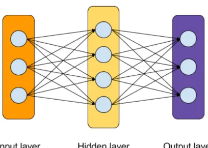
Several artificial neurons can further be interconnected to compose a neural network. Multilayer perceptron (MLP) is one of the most basic types of neural networks. A set of neurons with a common activation function is typically grouped into a layer. Multiple consecutive layers are then arranged into a neural network in a fully connected and feedforward manner. That is, all the neurons between subsequent layers are connected and output of a previous layer is fed as input to the next layer. A multilayer perceptron consists of three types of layers: input layer,

(16)

10

Figure 5: Basic model of an artificial neuron.

hidden layer, and output layer. Typically, there is only one input layer and one output layer, but the number of hidden layers can be larger than one. Figure 6

shows an illustration of a fully connected multilayer perceptron with one hidden layer. Formally, a one-hidden-layer MLP is a function f(·):

f(x) = φ2(W2φ1(W1x+b1) +b2) (3)

whereb1andb2 are bias vectors,W2 andW2are weight matrices,φ1(·) andφ2(·) are activation functions. This can be easily extended to represent multilayer perceptron with more hidden layers.

The width of each layer is determined by the number of artificial neurons in each layer and the depth of the network is determined by the number of layers. A multilayer perceptron with at least one hidden layer has universal approximation property [27]. That is, it can approximate smooth nonlinear mappings with any desired degree of accuracy provided that the hidden layers are sufficiently wide. In fact, a deep but narrow neural network is usually more efficient to approximate the same function.

2.3.2 Backpropagation

Artificial neural networks are typically highly non-linear and thus have no closed-form analytical solutions. Therefore, they are trained numerically in a supervised manner using backpropagation algorithm. The standard backpropagation algorithm [55] is essentially an instantaneous stochastic gradient algorithm.

A neural network can be seen as a function f(x|θ) of input x parameterized by its weight parametersθ. The goal to train a neural network is to find the θ such that

(17)

11

Figure 6: A fully connected multilayer perceptron.

the neural network can approximate a target functionf∗(x). That is, we want to find the θ that minimize the error between the desired output of the target function and the corresponding output of the neural network. Typically, the entire target function is unknown and only a set of training data is given, which can represent the function to some extent. Therefore, the error minimized during training is computed using the training data. In principle, the backpropagation algorithm tries to minimize the error and solve the weighs iteratively.

The mathematical description and derivation of the backpropagation algorithm are presented in many books (e.g. [22]) and thus we skip it. Here we briefly explain the steps of the standard backpropagation algorithm.

The first step of training is to initialize the weights of the network, for example to small random values. Then, a mini-batch of training data is sampled and the set of corresponding outputs of the network is calculated. The generated output predictions are compared with the corresponding ground truth training labels, and the training error is computed based on this comparison. Subsequently, the output error is propagated back through the network, and the gradient of each weighting parameter is calculated. Finally, the weights are updated using these gradients according to some specific rule. These steps except the initialization are repeated until the weight parameters converge.

The standard backpropagation algorithm converges slowly due to the use of the vanilla stochastic gradient descent, and bad choices for the learning rate can cause problems. Therefore, more efficient versions of backpropagation algorithm have

(18)

12 been proposed. One variant of it, Levenberg-Marquardt backpropagation (LMBP) algorithm [23, 45], uses a simplified version of Newton’s method for training to speed up the convergence. Some other variants, such as RMSProp [67] and Adam [34], use adaptive learning rate when updating the weights.

2.3.3 Convolutional Neural Networks

Convolutional Neural Networks (CNNs) [38] are variants of MLPs which are well-suited to process data with grid-like structure such as images. CNNs allow processing of large digital images, which is impossible using conventional fully connected MLP networks. They are extremely successful in practical applications, such as [19, 25, 36, 44, 52, 62]. Therefore, the development of convolutional networks has tremendously increased the popularity of deep learning.

Convolutional neural networks are specially structured neural networks using convolution operation in at least one layer, but typically using a stack of convolutional layers. Due to the use of convolution operation and weight-sharing, CNNs have translation invariance characteristics.

Convolutional neural networks were inspired by biological visual processes [28]. Animal visual cortex has many simple neurons acting as local feature detectors. Each neuron is responsible for a particular region of the visual field (i.e. its receptive field) and is sensitive to a certain type of stimulus. For example, some neurons respond to edges with a specific orientation. The receptive fields of neurons are restricted in size, but they overlap each other and cover the whole visual field. On top of these simple neurons, there are more complex neurons which pool the responses of the simple ones, and thus there is a feature hierarchy.

In convolutional neural networks, the function of the neurons in the visual cortex is mimicked by applying convolution operation between the image and filters. That is, the filter is slid over the image spatially to compute dot products. Filters are trained to represent different features. A sequence of convolutional layers approximates the feature hierarchy in the visual cortex. It has been shown that the lower layers closer to the input learn to recognize simple features of the image, such as edges and bright spots, and the higher layers closer to the output learn to represent complex features of the image, such as shapes and patterns.

Similar to an MLP, a CNN also has one input and one output layer, and several hidden layers in between. Typically, three types of layers are used in convolutional neural networks: convolutional, pooling and fully connected.

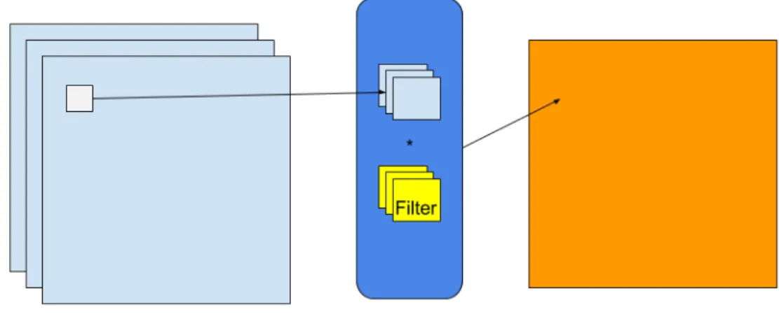
Typically, a convolutional layer consists of N filters of size Fx ×Fy ×d and

operates on an input volume of size Ix×Iy ×d. As mentioned before, each filter is

slid over the input volume spatially to compute dot products at each 2D position to yield an output volume of size Ox×Oy ×1. The output volume is called activation

map or feature map. This operation is also known as the convolution of two functions and thus we call the layer convolutional. Figure 7 is an example of convolution operation.

The size of the output feature map is determined by the strides of the convolution operation and the padding scheme. Strides determine the number of pixels with

(19)

13

Figure 7: Convolution operation.

which we slide the filter at a time, horizontally or vertically. In other words, in case the strides are both one, we move our filter one pixel at each step, and the convolution output for every pixel is computed. Convolution operation typically does not preserve the spatial size of the input volume. Thus, it is usually useful to add zero padding to the border of the input volume. Without padding, the size of the output volume is always smaller than the input if the size of the filter is larger than 1×1.

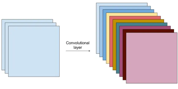
Finally, the N separate activation maps generated by theN filters are stacked along the 3rd dimension. This yields the final output of a convolutional layer of size

Ox×Oy ×N. A convolutional layer with ten filters is illustrated in Figure8.

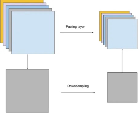
Pooling layers are used to make the feature representations smaller in size and thus more manageable, while preserving the most important information in them. As illustrated in Figure9, a pooling layer operates over each activation map independently to reduce the size of an input volume. This is done by sliding a small window across an input activation map and taking the maximum value or average value of the window at each step. These two different pooling schemes are known as max pooling and average pooling. As an example, max pooling is illustrated in Figure 10.

Since pooling reduces the size of the activation maps, it is a useful way to manage the computational complexity of the network. In addition, applying pooling makes the feature representations more invariant to small translations in the input. That is, the output remains almost the same when the input volume is slightly shifted.

(20)

14

Figure 8: A convolutional layer.

spatial information. Therefore, in many convolutional neural networks, pooling layers are simply replaced by convolutional layers with increased stride and this results in no loss in accuracy [64]. In this thesis, all the neural networks we use do not contain pooling layers.

Typically, fully connected layers are used at the end of a convolutional neural network, i.e., they are the final hidden layers. In principle, they are the same as layers in the aforementioned traditional MLPs, which connect every neuron in the previous layer to every neuron in the next layer. There are also convolutional networks without fully connected layers which are called fully convolutional networks (FCNs) [41]. Unlike traditional convolutional neural networks, they are able to manage different input sizes.

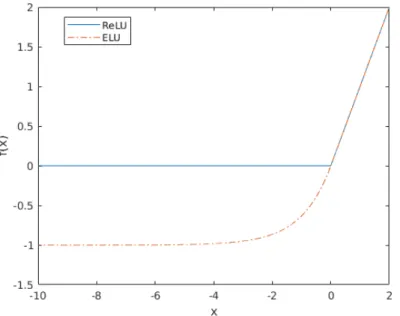
Activation functions are used between layers of a CNN to introduce nonlinearity. The rectified linear unit (ReLU) [50], which was first proposed for restricted Boltzmann machines, is currently the most commonly used activation function for convolutional neural networks. The main advantage of ReLU is that it can alleviate the vanishing gradient problem. Formally, ReLU is defined as:

f(x) = max(0, x) (4)

In this thesis, another activation function exponential linear unit (ELU) [8] is also used. It speeds up the learning in deep neural networks and has improved learning

(21)

15

Figure 9: A pooling layer.

Figure 10: Max pooling with 2×2 filter and stride 2.

characteristics compared to other activation functions. ELU is defined as:

f(x) =

(

x x >0

α(exp(x)−1) x≤0 (5)

where α >0. ReLU and ELU are illustrated in Figure 11.

(22)

16

Figure 11: The rectified linear unit (ReLU) and the exponential linear unit (ELU,

α= 1.0).

12. It is composed of a sequence of convolutional layers combined with pooling layers and one fully connected layer at the end.

Figure 12: An example of a convolutional neural network.

2.3.4 Fully Convolutional Networks

A fully convolutional network (FCN) [41] is a variant of the traditional convolutional neural network where all the learnable layers are convolutional, and thus it does not include any fully connected layers. By building the CNN fully convolutional with

(23)

17 upsampling layers inside the network, FCN could be applied to input of arbitrary size and output pixel-wise predictions efficiently. Note that the upsampling layers are not always needed, e.g., due to the use of dilated convolutions [72].

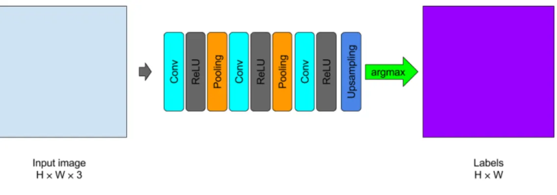
FCN was initially proposed for semantic segmentation task. Semantic segmenta-tion is the task of labeling each pixel in the image with one of the predetermined category labels. Its goal is to understand the image in pixel level. Before the existence of FCN, solving semantic segmentation with CNN was performed in a patch-based manner [7, 14]. As illustrated in Figure 13, in order to classify an image pixel, the traditional patch-based approaches use an image patch around a pixel together with the label of that pixel as a sample to train a CNN. This is known as patch-wise training. During test time, again an image patch is extracted around a pixel and fed into the CNN to produce a category label for that pixel. This is done for every pixel in the image to produce a dense final prediction. However, these approaches have several deficiencies. First, it requires much memory at test time. For example, if the size of the extracted image patch for each pixel is 40×40, the required amount of memory is 1600 times larger that of the original image. Besides, it is time-consuming and inefficient. Although the neighboring image patches are always overlapping, these approaches fail to reuse the shared features between patches, and this results in unnecessarily repeated computations. In addition, the size of the image patch limits the size of the receptive field. Typically, the size of the image patch is much smaller than the size of the entire image, and thus only local information without global context can be extracted, which affects the performance of the algorithm.

Figure 13: Patch-based sematic segmentation using CNN.

Unlike the patch-based approaches, FCN can be trained end-to-end simply using whole images and ground truth labels of the same size to make dense predictions for semantic segmentation efficiently at test time [41]. FCN and its variants have demonstrated a significant improvement in segmentation accuracy over traditional methods on standard datasets. Therefore, FCN has driven great breakthrough on semantic segmentation task and the idea of FCN has been successfully applied to other computer vision tasks.

(24)

18

Figure 14: Fully convolutional network.

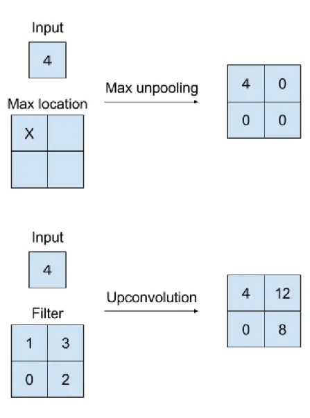
An example of the FCN structure is shown in Figure 14. Typically, a FCN-based model used for producing dense predictions is composed by successive convolutional layers with downsampling and upsampling inside the network. As discussed before, downsampling can be done by pooling layers or convolutional layers with larger stride value. In order to upsample the activation maps, upconvolution (sometimes called deconvolution) [52] and unpooling [73, 74] are introduced. Unpooling is the reverse operation of pooling which can enlarge the size of activation maps without learnable parameters. Similar to unpooling, upconvolution is the reverse operation of convolution. Here the reverse operation means the reverse of the forward and backward passes of convolution operation rather than the reverse of the convolutional effect (the mathematical deconvolution). In contrast to unpooling, the parameters of upconvolution can be learned. upconvolution and unpooling operations are illustrated in Figure 15.

2.3.5 Transfer Learning and Data Augmentation

Transfer learning is a machine learning technique for applying the knowledge gained during solving one problem to a related problem. Transfer learning with deep neural networks is usually performed by initializing the network with weights of a pre-trained network instead of random initialized ones and then finetuning the network [1, 53]. In practice, training an entire deep neural network from scratch with random initialization is usually not feasible, because of the insufficient size of a dataset. Even when the dataset is large enough, transfer learning can often help to boost generalization performance. Besides, training from scratch usually takes much more time. Therefore, transfer learning has become a common trend for training deep neural networks.

Typically, the weights are initialized from a classification network which is pre-trained on a very large dataset such as ImageNet [12]. Since the lower layers closer to the input learn to represent more generic features that are useful for almost all tasks,

(25)

19

Figure 15: Upconvolution (deconvolution) and unpooling operations.

we usually freeze the weights of the lower layers and only finetune or retrain the higher layers of the network. It has been shown that transferring the learned representations of classification networks to solve other tasks such as semantic segmentation is often useful.

Data augmentation is a common machine learning technique that can improve the generalization capabilities of machine learning models by increasing the amount of training data, and thus avoid them from overfitting and increase their accuracy at test time [70]. It has been proven to be useful for training deep neural networks, especially on smaller datasets. Typically, data augmentation generates new samples from the existing data by applying transformations. For example, we can translate, rotate, warp, flip, scale, and crop the images. Even more realistic and representative samples can be generated synthetically.

(26)

20

2.3.6 VGGNet

VGGNet [62] is a deep convolutional neural network architecture proposed by the Visual Geometry Group (VGG) from the University of Oxford. It explores the rela-tionship between the depth of the convolutional neural network and its performance. By increasing the depth to 16-19 layers, VGGNet shows significant improvement in accuracy. To reduce the number of parameters, only 3×3 filters are used in all convolutional layers. Compared to networks with fewer layers but larger filters, it has more non-linearities and fewer parameters. Two VGG based models VGG16 and VGG19 are shown in Figure 16. In the DSAC localization pipeline, the two CNNs are based on the VGGNet architecture.

2.3.7 DispNet

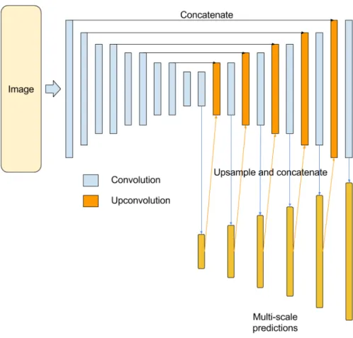
DispNet has been proposed in [47]. It is a fully convolutional neural network model with multi-scale predictions, which can be trained end-to-end to predict the dense disparity map from a pair of images. It adopts an encoder-decoder architecture where the encoder is used to compute abstract features and encode the global context, and the decoder recovers the original resolution by an expanding upconvolutional architecture [47]. Shortcut connections are added between the encoder and decoder to better preserve finer details of the input image. An example of the DispNet architecture is shown in Figure 17. In this thesis, our full-frame Coordinate CNN is based on the DispNet architecture.

(27)

21

(28)

22

(29)

23

3 Active Search Pipeline

In this chapter, we explain the state-of-the-art Active Search method [57, 58]. As described in Section2.2.1, it is a traditional keypoint based localization approach which solves the localization task by correspondence search. In this thesis, we primarily focus on improving neural network based methods. However, as we compare the neural network based methods to Active Search, we describe its pipeline in detail.

Active Search consists of a powerful prioritized keypoint search pipeline which is able to efficiently and effectively generates 2D-3D matches for pose estimation. It is called Active Search because the key component of it is an algorithm which can actively search for additional matches to improve the registration performance.

Figure 18: Active Search pipeline. Figure adapted from [58].

Active Search uses a visual vocabulary based prioritization scheme to accelerate the 2D-to-3D descriptor matching, where the SIFT [42] descriptors of the 3D models are clustered for faster indexing and estimating matching cost. Due to the quantization of the descriptor space, potential correct matches could be lost. Thus, a 3D-to-2D search scheme is used to reestablish these matches. Co-visibility of 3D points in the 3D model is further considered to speed up the matching. An overview of the Active Search pipeline is illustrated in Figure18.

(30)

24

3.1 Vocabulary-Based Prioritized Search (VPS)

As discussed in Section 2.2.1, there are two types of matching schemes: indirect and direct matching. Many previous methods adopt indirect matching to obtain efficiency. Although an indirect way of feature matching is faster than direct 2D-to-3D matching, the quality of the established correspondences in this way is much lower. Contrary to previous methods, the Active Search pipeline demonstrates the power of direct 2D-to-3D matching. The FLANN library [49] can be used to perform the 2D-3D matching between the query image descriptors and 3D points in the scene model represented by a kd-tree. If the ratio test of two nearest neighbors with the threshold set to 0.7 is passed, a potential 2D-to-3D match is accepted [56]. It has been shown that the quality of the matches established by the direct 2D-to-3D matching is higher [56].

However, the direct search based on kd-tree is time-consuming. In order to perform fast localization while preserving the quality of the matches, a better search scheme is needed. In fact, tree-based search spends most of the time on features which do not result in correspondences [56]. Therefore, we could first consider the most promising features which could lead to a match during the search by prioritizing the search using a meaningful strategy. And once enough matches have been established, the search can be terminated. To address this issue, the vocabulary-based prioritized search (VPS) scheme is proposed. VPS uses a visual vocabulary to estimate the matching cost of features. First, the 3D points associated with SIFT descriptors are clustered and assigned to a visual vocabulary consisting of a predefined number of visual words. This step is done offline. During test time, the extracted image features are also assigned to this set of visual words. Then, for each image feature, only the 3D points with which the same visual word is associated are the candidates for the nearest neighbor search. In this way, the number of feature descriptors assigned to the visual word of an image feature is proportional to the cost of finding the nearest neighbors of this image feature. Thus, the number of descriptors can be a good estimate of the matching cost to prioritize the search. VPS first processes the image features with lower matching costs. That is, features assigned to words with fewer points are evaluated first. The search stops when enough correspondences have been found. An illustration of VPS is shown in Figure 19.

3.2 Active Correspondence Search

Although the use of prioritization scheme results in far more efficient direct 2D-to-3D matching, VPS is not as robust as the search based on kd-tree. This is because of the quantization effects introduced by the use of a visual vocabulary. That is, if corresponding features have different visual words, the correspondence could not be established during the search. Therefore, the number of high-quality correspondences is limited. Using soft assignments could be a solution to recover the matches, but at the cost of computational efficiency. In contrast, active correspondence search is able to achieve this efficiently.

(31)

25

Figure 19: Vocabulary-based prioritized search(VPS). Figure adapted from [56].

Figure 20: Active correspondence search. Figure adapted from [57].

be recovered by active correspondence search through 3D-to-2D matching. When a 2D-to-3D match has been found by VPS, we know that the nearby region of the 3D point could also be seen in the query image. Thus, we can consider finding matches for the neighboring 3D points via 3D-to-2D search. Similar to VPS, searching for the nearest neighbors of a 3D point can be again accelerated by using a visual vocabulary. Unlike the one used for 2D-to-3D matching, the vocabulary for 3D-to-2D matching is supposed to be coarser to guarantee that each word is associated with enough image features, since the number of features in the query image is tremendously fewer than

(32)

26 that of a 3D model. This coarse visual vocabulary can be obtained efficiently by extending the fine one used for 2D-to-3D matching to a hierarchical vocabulary tree and extracting the high-level words. Using such a coarser vocabulary also leads to fewer quantization effects such that some of the lost matches during the 2D-to-3D search can be recovered.

The 3D-to-2D matching is actively triggered, and it shares the same prioritization scheme with the 2D-to-3D matching. Once a 2D-to-3D match has been found, K

nearest neighbors of the 3D point in 3D space are inserted to the prioritization scheme as candidates for 3D-to-2D matching. These 3D points are also prioritized by their matching costs, i.e., the numbers of features assigned to their visual words, together with other 2D features and 3D points that are already in the scheme. Once a 3D point is processed by the prioritization scheme, 3D-to-2D matching is performed rather than 2D-to-3D matching. Here, the same ratio test is used, and again the matching only considers the image features with the same visual word. Note that the search of K nearest neighbors of a 3D point in the 3D space is only performed when an 2D-to-3D match is accepted. There are also two other strategies to prioritize the search. One is to process all candidates for 3D-to-2D matching intermediately after a 2D-to-3D match is found. However, this can result in a large number of matches concentrated in a few parts of the image which should be avoided for pose estimation. The other one is to process all the 3D points only after all the 2D candidates are evaluated. In this way, active correspondence search could be useless, since enough correspondences can already be found before performing the 3D-to-2D matching.

3.3 Co-Visibility Information

Active correspondence search utilizes the assumption that the nearest neighbors of a found 3D point in the model can also be seen in the query image. However, this is not necessarily true. Therefore, the co-visibility information could be used to filter out unreliable neighboring points, and thus speed up the localization.

The co-visibility information can be approximated using the information obtained from the SfM pipeline. Since 3D points are generated from database images, two 3D points are unlikely to be seen at the same time in the query image if they are never seen together in a database image. Therefore, once the K nearest neighbors of a 3D point are found, only those have been co-visible in at least one database image are inserted into the prioritization scheme as candidates for 3D-to-2D matching. Other points are simply discarded. In this way, the correspondence search is accelerated.

The co-visibility information can also be used as a RANSAC pre-filter that can remove false matches before applying RANSAC. Once we have a set of 2D-3D matches ready to be fed into the RANSAC loop, we can connect two 3D points if they are co-visible in at least one database image. This results in a graph with multiple connected components, if we consider these 3D points as vertices of a graph. Points in different components should not be observed together in the query image. Therefore, only matches contained in the largest component should be used for pose estimation. By removing the false matches, the RANSAC-based pose estimation can be accelerated.

(33)

27 However, using only the database images results in merely an approximation to the true co-visibility information. Thus, the two filtering steps can also remove correct points and matches. In order to achieve better performance, cameras can be merged to obtain better and more continuous approximation of the true co-visibility relationship. For each image in the database, k images with the closest camera centers are found. Then the set of similar images are defined by the subset of thesek

images with relative orientation difference within 60◦. This results in a set of image clusters. When determining the co-visibility of two points, the images clusters are used instead. That is, if two points can be found together in at least one image cluster, they are considered co-visible. As a result, however, the filtering steps become far more computationally expensive. In order to reduce the running time, we can select only a minimal set of image clusters that covers all the database images using a greedy set cover algorithm.

(34)

28

4 DSAC Pipeline

In this chapter, we discuss the neural network based DSAC localization pipeline [3] which is based on the SCoRF pipeline [61] explained in Section 2.2.3. The DSAC pipeline is the main focus of this thesis, as we present two modifications to the DSAC pipeline in the next chapter.

As mentioned in Section 2.2.3, the original SCoRF pipeline requires the depth information during test time, which makes it limited. Instead of using a random forest to predict the 3D coordinates from a combination of RGB and depth features, the DSAC pipeline adopts a powerful deep neural network which can be discriminative enough without using the depth information. This enables the camera localization from RGB-only images.

Figure21 gives an overview of the DSAC pipeline. It consists of two stages, each of them containing a CNN. In the first stage, a Coordinate CNN is adopted to generate 2D-3D correspondences from a given RGB image. In the second stage, a differentiable RANSAC (DSAC) scheme is performed to determine the final pose estimate. Here several pose hypotheses are generated, and they are evaluated by a Score CNN. Due to the use of two CNNs and the differentiable RANSAC, the entire pipeline can be trained in an end-to-end manner.

Although the 6 DoF camera pose can also be directly regressed by a single CNN as demonstrated by PoseNet, the localization performance obtained in this way is inferior. Therefore, the intermediate step of generating 2D-to-3D correspondences contained in both the Active Search pipeline and the DSAC pipeline is critical for high-quality camera localization.

4.1 Differentiable RANSAC

Random sample consensus (RANSAC) algorithm [15] is one of the most famous tools in computer vision. It is a simple but powerful framework for model fitting when outliers are present. It is applicable to numerous problems in computer vision, such as pose estimation, camera calibration and 3D reconstruction, and often works well in practice.

RANSAC runs in a hypothesize-and-verify manner. Firstly, multiple hypotheses are generated by fitting models to randomly selected minimal subsets of data points. Then, these hypotheses are scored by how much they are consistent with the entire dataset. This is usually done by counting the inliers of each model, which fit the model within some error threshold. Finally, the hypothesis with the highest score is selected as the final output. Typically, an optional step can be performed to obtain a better estimation by refining the final output using all its inliers.

In the context of image-based localization, the RANSAC algorithm is usually used in combination with a PnP algorithm which can generate a camera pose estimation from a set of 2D-3D correspondences. A minimal subset of four correspondences is used to generate the pose in the case of known intrinsic parameters, and at least six correspondences are needed if intrinsic parameters are unknown. In this thesis, we consider the situation where the intrinsic parameters are known. Once a pose

(35)

29

Figure 21: DSAC pipeline. Figure adapted from [3].

hypothesis is generated, a 3D point can be projected onto the image plane using the hypothesized camera pose and the known intrinsic parameters. The reprojection error is then defined by the distance between its corresponding 2D pixel and the reprojected one. A 2D-3D correspondence is considered as an inlier of a pose hypothesis if the reprojection error is less than some threshold. The selected hypothesis is the one with the highest number of inliers and it can be further refined.

(36)

30 However, the traditional RANSAC algorithm is not differentiable, thus cannot be integrated into an end-to-end deep learning pipeline. If we want to propose an image-based localization pipeline which contains the intermediate step of predicting 2D-to-3D correspondences and at the same time can be trained end-to-end by directly minimizing the localization error (e.g. training PoseNet), a differentiable RANSAC is needed.

In order to make the traditional RANSAC differentiable, a differentiable score function, e.g., a Score CNN (explained in the next section), can be used instead of counting inliers. More importantly, the non-differentiable argmax operator which select the best hypothesis with the highest score should be replaced by a differentiable one. There are two different ways to achieve this. The first way (SoftAM) is to use soft argmax instead of argmax which turns the hard selection into a weighted average of all hypotheses. However, this results in learning a good average of hypotheses instead of learning to select the best one. Inspired by the policy gradient approaches in reinforcement learning, the second way is to preserve the hard selection but make it probabilistic. It is called DSAC (Differentiable SAmple Consensus). It has been shown experimentally that DSAC is less sensitive to overfitting than the first option for image-based localization. An overview of the traditional RANSAC and the two differentiable variants are shown in Figure 22.

Figure 22: A graphical representation of the traditional RANSAC and two differen-tiable variants of it. Figure adapted from [3].

Using this proposed differentiable RANSAC together with a Coordinate CNN and a Score CNN (discussed in the next section), an end-to-end trainable image-based localization pipeline is enabled, although componentwise training for good initialization is needed.

(37)

31

4.2 Coordinate CNN and Score CNN

As already mentioned, the DSAC pipeline contains two separate CNNs, a Coordinate CNN and a Score CNN. The Coordinate CNN is used to predict 2D-3D correspon-dences, and the Score CNN is for scoring hypothesis. Both CNNs are based on the VGGNet architecture [62].

The Coordinate CNN generates the 2D-3D correspondences as follows. For a 2D pixel in the image, a 42×42 image patch centered at the pixel is cropped and fed into the Coordinate CNN, and a 3D scene coordinate estimate is generated by this CNN. The location of the 2D pixel in the image and the predicted 3D position in the world space form a 2D-3D correspondence. During test time, only 40×40 pixels per image are randomly sampled and processed to reduce the running time. The sampling is done by first dividing the image into 40×40 cells and choosing a random pixel location for each cell.

The Score CNN predicts a score for a hypothesis from a reprojection error image. Once a pose hypothesis is generated from a minimal subset of the 40×40 2D-3D correspondences using a PnP algorithm, we can calculate the reprojection error for each of the 40×40 correspondences using this hypothesis. This results in a 40×40 reprojection error image for the hypothesis. To assess the quality of the hypothesis, the reprojection error image is directly fed into the Score CNN.

The detailed configurations of the Coordinate CNN and the Score CNN are described in Table 1. All layers expect the output layers in both the Coordinate CNN and the Score CNN are followed by a ReLU non-linearity. Unless indicated, all the convolutional layers are zero-padded with 1-pixel border. Unlike the original VGGNet architecture, there are no pooling layers in the networks. Convolutional layers with stride equal to 2 are used instead for downsampling.

Training the two CNNs jointly in an end-to-end fashion from scratch quickly reaches a local minimum, thus making the procedure useless. Hence, training the two components separately to provide a good initialization for end-to-end training is necessary.

The Coordinate CNN can be trained directly by minimizing the following loss:

losscoord(ˆy,y) =kyˆ−yk (6)

where y is the ground truth scene coordinate label of an image pixel and ˆy is the prediction of the Coordinate CNN. Here the Euclidean distance is used instead of the squared distance since it is more robust to outliers. The ground truth scene coordinates of a 2D pixel can be obtained using the 2D pixel coordinates, the depth value of the pixel and the camera intrinsic parameters. Hence, only image patches with valid depth information are sampled for training.

The Score CNN is trained using synthetically generated data. Given a training image, synthesized pose hypotheses can be generated by adding noise to the ground truth pose of this image. Then for each synthesized pose hypothesis, its reprojection error image can be computed using the predictions of the trained Coordinate CNN. Using the synthesized pose hypotheses and reprojection error images generated from training images and their ground truth poses, the Score CNN can be trained by

(38)

32 minimizing the following loss:

lossscore(ˆs, s) = |ˆs−s| (7)

where ˆs is the score predicted by the Score CNN ands is the ground truth score. To define the ground truth score, we need the loss between the ground truth pose and the pose hypothesis. It is given by:

losspose(ˆh,h) = max(∠(ˆθθθ, θθθ),kˆt−tk) (8)

whereh= [t, θθθ] and ˆh= [ˆt,ˆθθθ] are ground truth pose and pose hypothesis respectively. The camera rotations ˆθθθandθθθare in axis-angle form and the angular distance between them are measured in degree. The camera translations ˆt and tare measured in cm. Then the ground truth score is defined as:

s =−βlosspose(ˆh,h) (9)

where β is a hyperparameter that controls the broadness of the distribution after applying softmax to the scores of hypotheses. As illustrated in Figure 22, this distribution is used for weights in SoftAM or as the sampling distribution in DSAC. It is set to 10 in the original DSAC paper. Training in this way, the Score CNN learns to predict small scores for hypotheses with large errors and large scores for hypotheses with small errors.

Coordinate CNN Score CNN

42×42×3 RGB image patch 40×40×1 reprojection error image 3×3 conv, 3/64, s= 1, no padding 3×3 conv, 1/32, s= 1

3×3 conv, 64/64, s= 2 3×3 conv, 32/32, s= 2 3×3 conv, 64/128, s= 1 3×3 conv, 32/64, s= 1 3×3 conv, 128/128, s = 2 3×3 conv, 64/64, s= 2 3×3 conv, 128/256, s = 1 3×3 conv, 64/128, s= 1 3×3 conv, 256/256, s = 1 3×3 conv, 128/128, s= 2 3×3 conv, 256/256, s = 2 3×3 conv, 128/256, s= 1 3×3 conv, 256/512, s = 1 3×3 conv, 256/256, s= 2, no padding 3×3 conv, 512/512, s = 1 3×3 conv, 256/512, s= 1 3×3 conv, 512/512, s= 2, no padding 3×3 conv, 512/512, s= 2

FC 2048/4096 FC 512/1024

FC 4096/4096 FC 1024/1024

FC 4096/3 FC 1024/1

Table 1: Configurations of Coordinate CNN and Score CNN.

4.3 End-to-End Training

After initializing the Coordinate CNN and the Score CNN with componentwise training as described in the previous section, the entire DSAC pipeline can be trained

(39)

33 end-to-end. The differentiable loss of the entire pipeline is the loss between the ground truth camera pose and the estimated pose which can be computed according to Equation8. However, some parts of the pipeline are still not directly differentiable. They are the pose hypothesis generation step using the PnP algorithm [35] and the final iterative pose refinement step.

For the pose estimation using the PnP algorithm, the derivatives can be calculated using central differences [17, 39]. The final refinement step is performed by iterating inlier sampling and pose estimation multiple times. Since it contains hard inlier selection operation, it is non-differentiable. However, because of the large number of inliers that are chosen, the refined poses typically change smoothly with regard to the scene coordinate prediction. Therefore, the derivatives can be again calculated using central differences by considering the refinement step as a whole. In order to make the derivatives more stable, refinement step is stopped if the number of inliers found is less than 50. In addition, to calculate the central differences efficiently, only 1% of the scene coordinates are sampled and the gradient is corrected by multiplying it by 100.

(40)

34

5 DSAC Variants

In this chapter, we present two modifications to the DSAC pipeline which is described in the previous chapter. First, we propose to discard the use of the Score CNN and the differentiable RANSAC, meaning that instead of first training the two CNNs separately and fine-tuning the entire pipeline end-to-end, we only train the Coordinate CNN to predict the 2D-3D correspondences and use the traditional RANSAC which is non-differentiable and contains no learnable parameters to generate the final poses. The second modification is that instead of performing scene coordinate regression in a patch-based manner, we propose to use a fully convolutional Coordinate CNN which takes the whole image as input and efficiently produce correspondingly-sized dense scene coordinate predictions.

5.1 Non-Differentiable RANSAC

As explained in Section 4.2, in the original DSAC pipeline, the Score CNN is used to regress the scores of hypotheses from their reprojection error images instead of directly scoring them by counting inliers. This makes the scoring function differentiable, and thus it enables the end-to-end training of the entire pipeline together with the differentiable hypothesis selection operation and the Coordinate CNN. However, while compared to the scoring scheme that uses only the number of inliers, the CNN-based score function has more discriminative power such that it can utilize more information from a reprojection error image to assess the quality of the hypothesis, it can easily overfit the training data. Furthermore, the componentwise training of the Score CNN is performed by using synthetically generated data. The pose hypotheses are generated by adding noise to the ground truth poses of training images, and the reprojection error images of these poses are generated using the scene coordinate predictions of the trained Coordinate CNN. Hence, the quality of the Score CNN is highly correlated with the quality of the Coordinate CNN and the density of training poses in the whole pose space. This can result in even more severe overfitting. For example, it is possible that during training the synthesized hypotheses with smaller errors have worse reprojection error images due to the quality of the Coordinate CNN, and thus the Score CNN learns to predict higher scores from worse reprojection error images. At test time, if the test image is similar to the training images, it will still work. However, if the test image is far from the training images, the generated hypotheses with better reprojection images which are actually the ones with smaller errors will not be recognized by the Score CNN and small scores will be given to them. Therefore, we argue that the use of the Score CNN can lead to worse performance for scenes with few training images or that are difficult for the Coordinate CNN (e.g. scenes contain repeated structures).

On the other hand, the conventional RANSAC has been already proven to be robust for many computer vision applications. Although the scoring using inlier count is simple and not as discriminative as a CNN-based score function, it can generalize well to different scenarios and is not sensitive to the size of training data and the quality of the Coordinate CNN. Therefore, we propose to use the conventional