Department of Economics
University of St. Gallen
Forecasting Implied Volatility Surfaces
Francesco Audrino and Dominik Colangelo
Editor:
Prof. Jörg Baumberger
University of St. Gallen
Department of Economics
Bodanstr. 1
CH-9000 St. Gallen
Phone
+41 71 224 22 41
Fax
+41 71 224 28 85
Email [email protected]
Publisher:
Electronic Publication:
Department of Economics
University of St. Gallen
Bodanstrasse 8
CH-9000 St. Gallen
Phone
+41 71 224 23 25
Fax
+41 71 224 22 98
http://www.vwa.unisg.ch
Forecasting Implied Volatility Surfaces
Francesco Audrino and Dominik Colangelo
Author’s address:
Prof. Dr. Francesco Audrino
Institute of Mathematics and Statistics
Bodanstrasse 6
9000 St. Gallen
Tel.
+41 71 224 2431
Fax
+41 71 224 2894
Email [email protected]
Website www. istituti.usilu.net/audrinof/web/
Author’s address:
Dominik Colagelo
Swiss Finance Institute
Via Buffi 13
CH-6904 Lugano
Tel. +41 58 666 44 92
Fax +41 58 666 47 34
Abstract
We propose a new semi-parametric model for the implied volatility surface, which
incorporates machine learning algorithms. Given a starting model, a tree-boosting algorithm
sequentially minimizes the residuals of observed and estimated implied volatility. To
overcome the poor predicting power of existing models, we include a grid in the region of
interest, and implement a cross-validation strategy to find an optimal stopping value for the
tree boosting. Back testing the out-of-sample appropriateness of our model on a large data
set of implied volatilities on S&P 500 options, we provide empirical evidence of its strong
predictive potential, as well as comparing it to other standard approaches in the literature.
Keywords
Implied Volatility, Implied Volatility Surface; Forecasting; Tree Boosting; Regression Tree;
Functional Gradient Descent
JEL Classification
1
Introduction
Despite the discrepancy between the Black and Scholes (BS) theory and reality, the concept of implied volatility surfaces (IVS) is still very popular. The mapping from observed market prices to implied volatilities (IV) is used as a way to make option prices more comparable. IVs of options are calculated and stored in financial databases. Market makers, traders, and risk managers rely on IV to calibrate their pricing models.
In efficient markets, new information has an instantaneous influence on option prices, which reflect expectations about future prices of the underlying stock. Hence IV can be seen as predictor for future volatility. This concept was formalized by Dupire (1994). Conditional on the market level of the underlying stock at some future date, T, which is set as equal to K, and conditional on the available information up to time t, the market’s expectation of the instantaneous volatility under the risk-neutral measure is defined as the local volatility. The Dupire formula represents local volatility as a function of observed call prices and their derivatives. Under certain conditions, IV can be thought of as an average of local volatility through the lifetime of the option.
Classical approaches assume that instantaneous volatility is a deterministic function in spot price and time. This implies that local and instantaneous volatility coincide. Dumas, Fleming, and Whaley (1998) find that estimated parameters are highly unstable over time, allowing only for short time predictions. As Poon and Granger (2003) point out, classical time series-based methods do not perform well in predicting instantaneous volatility. In Chapter 6 they also report that forecasting the instantaneous volatility based on option implied standard deviation has superior performance across different assets and over quite long forecast horizons (up to three years). This approach needs a strategy to decide which point on the IVS or which weighting scheme should be used to obtain a forecast of the instantaneous volatility, used as input in a option pricing framework.
In contrast to previous approaches, we model the whole implied volatility surface in order to price options simultaneously via BS formula as mapping from option prices to IV. Gon¸calves and Guidolin (2005) combine a cross-sectional approach similar to that of Dumas, Fleming, and Whaley (1998) with vector autoregressive models, but with exactly this idea in mind. The findings are mixed, and provide only a good in-sample fit, but questionable out-of-sample performance. Even the more complex and computational demanding dynamic semi-parametric factor model (DSFM) of Fengler, H¨ardle, and Mammen (2007) has quite limited predicting power. In a comparison of the one-day prediction error, the DSFM performs 10 percent better than a simple sticky-moneyness model, where IV is taken to be constant over time at a fixed moneyness.
Following this direction, we propose a new semi-parametric model based on an additive expansion of simple fitted regression trees, which can be easily estimated using boosting tech-niques. Any starting model can be enhanced with the help of our framework by including exogenous factors. The relevant ones are chosen automatically by the regression trees used in our model to minimize the residuals of observed and estimated IV. In this way, it fits the IVS in-sample to any accuracy by construction. An additional contribution of this paper is a method which improves the out-of-sample prediction of the IVS and which can handle very high values of IV, of both in- and out-of-the-money options.
We explore the out-of-sample performance of our model on a large data set of S&P 500 options, along the way collecting strong empirical evidence of the predictive potential of our model. We also compare our to a number of other approaches recently proposed in the literature on IVS. For example, our method can considerably improve on average IV forecast accuracy of a simple sticky-moneyness approach or an ad-hoc Black and Scholes model when focusing on forecasting horizons up to some months.
The paper is organized as follows. Section 2 briefly discusses the concept of IV and defines the IVS. Section 3 presents our model in detail and Section 4 contains the empirical part. We fit our model to S&P 500 option data, trying not to lose any information by filtering. We then discuss the included exogenous factors and compare the performance of our model in terms of IV forecast accuracy with a number of other approaches, including a simple sticky-moneyness model, an ad hoc BS model, and a principal component analysis (PCA) based model. Section 5 summarizes the main results and concludes.
2
Implied volatilities
Option pricing in the BS framework is easy and straightforward. Given the price of the underlying (non-dividend paying) stock St, the option’s strike price K, the risk-free interest
rate r, and the expiry date T of the option, the fair price of a call option CBS
t , and a put
option PBS
t at timetare given by:
CBS t (St, K, T, σ, r) = Stφ(d1)−Ke−r(T−t)φ(d2) (1) PBS t (St, K, T, σ, r) = Ke−r(T−t)φ(−d2)−Stφ(−d1) (2) where: d1 = log St K +r+σ2 2 (T −t) σ√T−t d2 = d1−σ √ T−t
The underlying stock price is assumed to follow a geometric Brownian motion with constant driftµand constant instantaneous volatility σ:
dSt
St
=µ dt+σ dWt
This implies that the log return process of St has a normal distribution:
log ST St ∼N (µ−1 2σ 2)(T−t), σ2(T −t)
The only unobservable variable in this setting is the most crucial one: the volatility σ. By equating the observed market price (Ct, Pt) of an option with the BS price (CtBS, PtBS) and
monotonicity of the BS price inσ. According to the BS assumptions, this implicitly calculated volatility should be constant. Unfortunately, it can be easily shown empirically that options with different strikes and expiry dates have an inconstant IV, not only contemporaneously (existence of volatility smiles/smirks), but also over time.
In fact, implied volatility should be considered as a mapping from time, strike, and expiry date. The mapping:
˜ σIV
t : (K, T)7−→σ˜tIV(K, T) (3)
is called the implied volatility surface (IVS). Plugging St, K, r, T, and ˜σIVt (K, T) back in the
BS formula leads (by definition of IV) to the observed market price. So, knowing the price of the underlying stock, the risk-free interest rate, and the IVS at timetis equivalent to knowing the market price of any option with any given contract characteristic1. The mapping allow
us to compare two options, even with different characteristics. The one with the higher IV is priced relatively higher compared to the other one with lower IV.
As it is usually done in the IV literature, we also describe the IVS in relative coordinates. Let m =K/St denote the moneyness and τ = T −t the time to maturity. The IVS is then
given by: σIV t : (m, τ)7−→σ IV t (m, τ) = ˜σ IV t (m·St, t+τ) (4)
3
Method
As a starting point, let us consider the non-parametric least square kernel (LSK) smoothing estimator for the IVS introduced by Gouri´eroux et al. (1995):
ˆ σIV(m t, τ) = arg min ˜ σ n X i=1 (cti−c BS( ·,σ˜))2ω(mti)K1 mt−mti h1 K2 τ −τti h2 (5) The observed call prices are normalized by the price of the underlying stock, andct=Ct/St,
andcBSis the BS formula in terms of moneyness, that isCBS
t (St, K, T, σ, r) =StcBS(m, τ, σ, r).
No inversion of the BS formula is needed, because observed market prices act as inputs. The estimate for a particular point on the IVS is given by the minimum of the loss function, in this case, the weighted sum of least squares. K1 andK2 are univariate kernel functions with
bandwidths of h1 and h2 respectively. ω(m) denotes a uniformly continuous and bounded
weight function, depending on m.
Fengler (2005) presents a summary of possible weight functions from the early literature on IV. Gouri´eroux et al. (1994) prove that under some weak conditions, the LSK estimator ˆ
σIV(m
t, τ) converges in probability to the true volatility of the underlying asset price process.
Out-of-sample prediction is the greatest disadvantage of smoothing techniques, because kernel functions explicitly depend on observed data. Nevertheless, the LSK method appears a quite attractive way of modeling the IVS in-sample. It belongs to the class of kernel M estimators and is therefore not only consistent, but also asymptotically normal.
1
It may be desirable to incorporate several features in our model. First, for our purpose it is convenient to use directly implied volatilities in the quadratic loss function instead of normalized observed market prices. Second, the weight function will also more explicitly take time to maturity into account, and guarantee good predicting power in certain areas of interest, for example, the area where in-the-money options will shortly expire. Third, we want to overcome the above-mentioned out-of-sample prediction problem.
3.1 Model
Given the remarks above, this section describes the model by which we propose to estimate and forecast the dynamics of IVS. The next section introduces an easy and computationally feasible algorithm which can be used to estimate the model.
Our approach relies on a fixed grid in the (m, τ) domain, which should be laid over the region where forecasts of the IVS are to be calculated. Using the following indexing:
[1] := (m(1), τ(1)), [2] := (m(2), τ(1)), ..., [Nm] := (m(Nm), τ(1)), [Nm+ 1] := (m(1), τ(2)), [Nm+ 2] := (m(2), τ(2)), ..., [2·Nm] := (m(Nm), τ(2)), .. . [(y−1)·Nm+x] := (m(x), τ(y)), x∈ {1, ..., Nm}, y∈ {1, ..., Nτ} (m(1)< m(2)< ... < m(Nm), τ(1) < τ(2) < ... < τ(Nτ)) a grid with grid points GP ={[1],[2], ...,[Nm ·Nτ]} is obtained.
Starting from an initial model, additive expansions in the form of regression trees1 with a small number of leaves (typically L = 2,3 or 5) are used to fit the data. To overcome the poor predictive power of off-the-shelf regression trees, the grid must be laid over the region where the IVS is to be predicted. This helps to obtain reasonable forecasts, because the model is fitted via kernel weighting in such a way that the focus is set to the region of the grid. Observations distant from grid points have less influence in the loss function. In the same manner of (5), we focus on a quadratic loss function which depends directly on implied volatilities: L(σIV ,σˆIV ) = (σIV −σˆIV )2.
The empirical local criterion to minimize over the grid specified before is then defined by: Λgrid= N X t=1 Lt X i=1 X [g]∈GP (σIV ti −σˆ IV ti) 2 wt(i,[g]), (6)
with weights specified by:
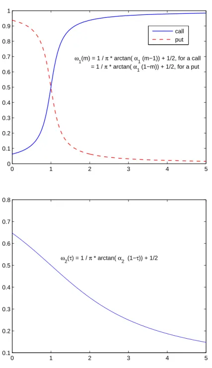
wt(i,[g]) =ω1(mti)·ω2(τti)·K m (x)−mti h1 ,τ(y)−τti h2 , (7)
In the above equation, the different quantities are specified by: [g] = (m(x), τ(y))∈GP, x∈ {1, ..., Nm}, y∈ {1, ..., Nτ} K(u, v) = 1 2π ·e −1 2(u 2+v2) ω1(mti) =
1/π·arctan(α1(mti−1)) + 1/2, if option i is a call
1/π·arctan(α1(1−mti)) + 1/2, if option i is a put
ω2(τti) = 1/π·arctan(α2(1−τti)) + 1/2
(mti, τti, σtiIV), i∈ {1, ..., Lt} denote the observations of moneyness, time to maturity, and
IV at day t. The daily number of observations Lt is varying over time, when new options
are issued or when others expire. In contrast, the grid points are fixed, and a model can be evaluated at those grid points at any point in time. This makes it possible to estimate a (Nm·Nτ)-dimensional time series of IV on the fixed grid.
The weighting function (7) consists of three factors. The first is ω1, taken from Fengler
et al. (2007), with slight corrections such that out-of-the-money options have more influence than in-the-money options. The second one is ω2, and depends on the time to maturity. It
was chosen to reduce the influence of options which expire far in the future, and to increase the importance of options that are due soon.
The choice of the kernel is less important as the choice of the grid. To compare the efficiency of different initial estimation models, a Gaussian kernel with constant stepwidth of h1 =h2 = 0.5 was chosen. α1 is set to 5 andα2 to 0.5. From a numerical point of view, it is
convenient to normalize the weighting function in such a way that:
Lt X
i=1
wt(i,[g]) = 100
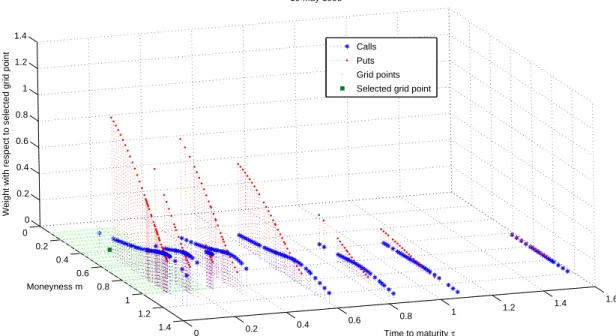
for every [g]∈GP and t, because the product of three small factors can become very small. An illustrative example of the weights with respect to a selected grid point on 19 May 1998, as well as the weight functions w1(m) and w2(τ), are shown in Figure 1 and 2.
[Figure 1 about here.] [Figure 2 about here.]
3.2 Estimation procedure
Tree boosting is a simple version of the functional gradient descent (FGD) method2, using regression trees as base learner and a quadratic loss function. In this case, the negative gradients are linear in the implied volatilities, and each FGD step reduces to an iterative refitting of generalized residuals.
A cross-validation scheme is needed to prevent the model from over-fitting. The first 70 percent of the days in the training data are considered to be a learning sample, and
the remaining 30 percent as a validation sample. The model is fitted on the aggregated IV observations in the learning sample only. The more additive components in the expansion there are, the smaller the error in the learning sample becomes. It tends to zero as the number of iterations increases, but this generally accompanies a worsening predictive power. The empirical local criterion (6) was tailored to highlight importance of prediction errors in the grid region. The addition of expansions is ceased when the empirical criterion takes its minimum on the validation sample. Slow convergence is desired in order to find the optimal number of iterations M, but using the negative gradient of the loss function in (6):
X [g]∈GP 2(σIV ti −σˆ IV ti)wt(i,[g])
requires too many iterations (>500). To make computation feasible, we use the un-weighted residuals in growing the additive expansion (see step 2 of the algorithm below). The learning rate can be further controlled by introducing a small shrinkage factor ν >0.
Taking all the above considerations into account, the following algorithm is proposed to estimate the IVS.
Algorithm: Tree-boosting for Implied Volatility Surfaces (treefgd)
1. Fit initial model F0(m, τ,cp flag,factors) to the datat∈ {1, ..., N}, i∈ {1, ..., Lt}:
ˆ σIV,0
ti = Fˆ0(mti, τti,cp flagti,factorst) (8)
= Fˆ0c(mti, τti,factorst)1I{cp flagti=call}+ ˆF
p
0(mti, τti,factorst)1I{cp flagti=put}, where “cp flag” indicates the type of the option (call or put), and “factors” indicates that relevant exogenous factors may be included as additional predictor variables fitting the model (see Section 4.3 for more details).
2. Forj= 1, ..., M:
(a) Fort= 1, ..., N, i= 1, ..., Lt compute:
residualti=σtiIV−σˆ
IV,j−1
ti
=σIV
(mti, τti,cp flagti)−Fˆj−1(mti, τti,cp flagti,factorst).
(b) Fit a regression tree withL leaves to the targets residualti:
d
tree(m, τ,cp flag,factors) =tree[c(m, τ,factors)1I
{cp flag=call}
+tree[p(m, τ,factors)1I
{cp flag=put}.
(c) Update: ˆ
Fj(m, τ,cp flag,factors) = ˆFj−1(m, τ,cp flag,factors)+ν·tree(d m, τ,cp flag,factors),
3. Choose ˆM such that Λgrid( ˆFMˆ) is minimal over the validation sample. Use only the
learning sample for fitting the models in Steps 1 and 2.
4
Application
4.1 Data
Implied volatilities of call and put options with different strikes and maturities on the S&P 500 index are analyzed for this project. The data ranges from 4 January 1996 to 29 August 2003 and consists of 777,887 observations on 1,928 days. Figure 3 shows the prices and log-returns of the S&P 500 index under consideration.
[Figure 3 about here.]
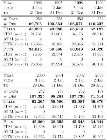
There are approximately 400 observations of IV per day on average over the whole sample. They appear in a so-called string structure, which means that usually only options with a few standardized time to maturities are traded, but for each τ there are many different strikes. The observations of the next day contain yesterday’s options where the times to maturities are net of 1/365 and the moneyness of each option has changed because the underlying has also. Tables 1 and 2 show summarized statistics of the option data under investigation.
[Table 1 about here.] [Table 2 about here.]
We fitted our model to 10 different sub-samples. Half are 250 days long, the other half 60 days. They are chosen to occur before five special days of interest, where – from today’s perspective – a more or less heavy structural break is expected to happen. On 7 August 1998 two bomb attacks on US embassies in Africa occurred. The impeachment trial of President Clinton was opened in the senate on 7 January 1999. The first date for which we have IVS observations in our sample after President Bush’s oath of office and the disruption caused by the unclear outcome in the presidential election 2000 is 22 January 2001. 17 September 2001 is six days after the 11 September terrorist attacks, and 20 March 2003 marks the official beginning of the military campaign against Iraq. The explicit sub-samples are summarized in Table 3.
[Table 3 about here.]
The 10 sub-samples end four to 25 days before these special days of interest. Our goal is to attain 60 days out-of-sample predictions of the IVS, such that we can compare the observed IV with the predicted one, before and after a supposed structural break. The accuracy of fit is measured by evaluating our fitted model at the exactly same (m, τ) locations as observed, and finally by calculating the sum of squared residuals (SSR) and the value of the empirical criterion.
4.2 Keeping extremal IV in the sample
The IVS literature often contains only out-of-the-money options (OTM,m >1 for call,m <1 for a put) for consideration. It is claimed that those options contain the most information about the IVS; see Cont and da Fonseca (2002), for example. Another argument for excluding in-the-money (ITM) options is that they contain a liquidity premium3.
Gon¸calves and Guidolin (2005) apply five exclusionary criteria to filter their IVS data. They exclude thinly traded options, options that violate at least one basic no-arbitrage condi-tion, options with fewer than six trading days to maturity or more than one year, options with moneyness smaller than 0.9 and larger than 1.1, and finally, contracts with price lower than three-eighths of a dollar. Cassese and Guidolin (2005) investigate the pricing efficiency in a bid-ask spread and transaction cost framework. They find a frictionless data set by dropping 51 percent of the original observations.
The model proposed in this study should be able to handle all options in the database, including ITM options, at-the-money (ATM) options, and even those with very high IV.
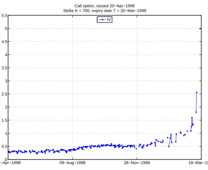
The option with the highest IV in the sample was a call issued in 20 April 20 1998 with a strike of 700 and expiry date 20 March 1999. With three days to maturity left, it reached an IV of 4.99, which is extremely high compared to the mean IV of the whole sample, which was 0.2748. Figure 4 shows the time series plot of the IV.
[Figure 4 about here.]
The S&P 500 started at $US1,123.7 (m= 0.6229), ended at $US1,299.3 (m= 0.5388), and was never below $US957.3 (m= 0.7312) during this period; hence this call option was always ITM. It is known that ITM calls and OTM puts are traded at higher prices compared to corresponding ATM options in general, but when the expiry date nears, observed prices, and IV reacts violently, as seen in the previous example. So, excluding these strangely behaving options from the sample should help any model to perform better, but might neglect the reality of having such high IV values. Regardless of what causes very high IV (miscalculation, wrong risk-free interest rate, illiquidity and so on), removing such extreme IV values would lead to a loss of information that may be important for prediction. There are 6,449 options with IV>1 in the sample, 4,748 of which are call options (3,743 ITM; 1,005 OTM), and 1,701 put options (1,093 ITM; 608 OTM). The mean of those options with IV>1 is 1.6517.
An essential feature of our proposed model is to be able to handle options shortly before the expiry date, where small measurement errors of the noisy prices of the underlying could lead to large errors in the IV for options away from the money (see, for example, Hentschel, 2003). The weighting function (7) guarantees that extremal IV can be kept in the sample and controls their influence.
4.3 Factors
Unlike its behavior in the theoretical BS framework, the option price depends on its contract characteristics, the price of the underlying, and the risk-free interest rate. However, exogenous factors can also be taken into account. Our proposed model allows for an arbitrary number
of exogenous factors, because the algorithm for constructing the additive expansion chooses automatically suitable L−1 split variables in order to set up a tree with L leaves. It is prudent to consider lagged factors, with lags both in the past and in the future4. The factor time series can easily be modeled and forecasted with standard time series approaches5. The
split variables are finally chosen among the location variables m, τ, the lagged prices of the underlying, and the lagged factors.
Possible exogenous factors to consider are implied asset prices (Garcia, Luger, and Renault, 2003), the bid-ask spread, net buying pressure (Bollen and Whaley, 2004), trading volume, other stock or index returns, and interest rates. In this study, the three-, six-month, and the one-, three-, five-, and 10-year treasury constant maturity rates6 represent the term structure
of interest rates. The set of exogenous factors contains these and also the prices of 18 options with different characteristics (call and put, m ∈ {0.8,1,1.2}, and τ ∈ {30,60,90 days}, see Table 4), calculated according to the model of Heston and Nandi (2000) in a rolling window of 500 days, shifted every 30 days.7
[Table 4 about here.]
The Heston and Nandi (2000) model is based on an asymmetric GARCH process for the spot asset price, and offers closed-form solutions for option prices. Including these 18 Heston-Nandi-GARCH (HNG) factors in the set of exogenous factors acts as a guidance for our model. Intuitively, if the estimation procedure chooses as splitting variable a HNG factor, it implies realigning the minimization of the residuals of observed and estimated IV to option prices calculated with the analytical Heston-Nandi pricing formula.
4.4 Relative importance of predictor variables
Similar to what is produced by interpreting boosting algorithms, we here address the question about the relevance of the different predictors in our real data application. As mentioned earlier, the model is fitted on 10 different sub-samples. Cross-validation on each reveals
P10
i=1Mˆi = 920 additive expansions in total. An additive expansion consists of two regression
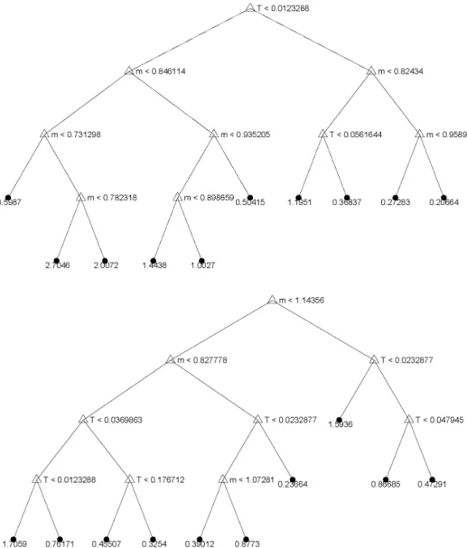
trees with L = 5 leaves, one for the calls and one for the puts. This leads to a total of 2·920·(L−1) = 7,360 split variables. Two illustrative examples of regression trees estimated by our procedure are shown in Figures 5 and 6.
[Figure 5 about here.] [Figure 6 about here.]
The location parameters m and τ were selected as splitting variables 5,674 times (77 percent), and are by far the most important predictors. Lagged treasury constant maturity rates were chosen 404 times (5.5 percent). More relevant for prediction of the IVS are lagged HNG factors; they were chosen 1,227 times (16.7 percent). Forecasting information included in lagged close prices of the underlying appears negligible; they were chosen only 55 times (0.8 percent).
Looking at the time lags that have been chosen reveals an interesting insight, and confirms that taking into account both past and future estimated lagged exogenous factors was indeed wise. Past lagged close prices, DGS and HNG factors were chosen 747 times, whereas future lagged factors were selected 716 times, and contemporaneous factors only 223 times.
4.5 Comparisons
The first five sub-samples introduced in Section 4.1 are 250 days in length. Our model is fitted on them, using a linearly spaced 15 ×15 grid with values from m= 0.2 to 2 and from τ = 3651 to 3. Achieving adequate 60-day forecasts over the whole (m, τ) domain with only 60 days of observed IVS to fit the model on is impossible, so we were satisfied with at least good predictions of the soon-expiring in-the-money calls. Hence a linearly spaced 20×20 grid with values from m = 0.1 to 1 and from τ = 3651 to 36590 is used for the second five sub-samples in Section 4.1 of 60 days in length. Before presenting the results, we briefly introduce the competing methods to the model proposed in Section 3.1 (treefgd).
4.5.1 Ad hoc BS model (adhocbs)
Dumas, Fleming, and Whaley (1998) proposed a framework in which local and instantaneous volatility coincide, because volatility is considered to be deterministic. Several functions of quadratic form are estimated by minimizing the sum of squared errors between the reported option prices and those obtained by solving the forward partial differential equation of Dupire (1994): 1 2σ 2(K, T)K2∂2C ∂K2 = ∂C ∂T
with the initial conditionC(K,0) = max(FT−K,0), whereFtdenotes the forward price of the
underlying at timet. Also, the option priceC is expressed as a forward price to the maturity date of the option. A goodness-of-fit test showed that the best parametrization is:
σ(K, τ) = max(0.01, a0+a1K+a2K2+a3τ +a4Kτ). (9)
Three exclusionary criteria are applied to the data. Dumas, Fleming, and Whaley (1998) eliminate options withτ <6 days andτ >100 days from their sample. Options with a forward moneyness K
Ft >1.1 and< 0.9 are also excluded. Option prices during the last half hour of trading are not taken into account.
We use an adapted version of the ad hoc BS model to compare it with our method. In analogy to (9), we fitted:
σIV
ti =at0+at1mtiSt+at2(mtiSt)2+at3τti+at4mtiStτti+ǫti (10)
by least square, using all Lt observed data points on day t. In case of negatively estimated
IV, values are set to 0.01. The a coefficients estimated on the last day in the data sample are used to calculate the IV out-of-sample. A second version of the ad hoc BS model is daily updated and uses previous day’s observed data to estimate theacoefficients and today’s IV.
4.5.2 Sticky moneyness model (stickym)
The sticky moneyness model is a ‘na¨ıve trader model.’ It assumes that IV is constant at fixed moneyness. To calculate the IV on a future datetat location (mt, τt), the following procedure
is implemented:
Data griddingOn a reference day ˜t < t, Delaunay triangulation-based cubic interpolation is used to fit the IVS as a function of the location parameters (m, τ) to the observed data
{(m˜ti, τ˜ti, σti˜IV)|i= 1, ..., L˜t}on that day.
Table lookup The function found before is evaluated at the sites:
{(mt, τ)|τ ∈ {100 linearly spaced values from min(τti˜) to max(τ˜ti), i= 1, ..., L˜t}}
to obtain a table. Because IVt is assumed to be equal to IV˜t for (mt,·), the tabulated IV
values can be used to calculate IVtat (mt, τt) via piece-wise cubic Hermite interpolation. This
method preserves monotonicity and the shape of the data. No extrapolation is conducted, and out-of-range values are set to the average IV on day t.
4.5.3 Principal components analysis (pca)
Our method is used to calculate the IV in-sample for call and put options separately on a linearly spaced 20×20 grid fromm= 0.2 to 2 and fromτ = 1/365 to 3. The 800-dimensional time series obtained in this way mirrors the IVS, where each component covers the in-sample evolution of the IV for a specific option characteristic (m, τ,cp flag). Principle components analysis (PCA) is then conducted after dividing each component by its standard deviation. The number p of considered principal components is determined in such a way that at least 90 percent of the variance of the standardized data is explained by them, usuallyp≤6.
To get an out-of-sample prediction for the IVS, the p considered principal components are forecasted within an ARMA-GARCH framework. The data is then transformed back in its original coordinate system. A Delaunay triangulation-based cubic interpolation is used to calculate the IV at any (m, τ,cp flag) location between the grid locations.
4.5.4 Out-of-sample results
We measured goodness-of-fit of the different competitors with respect to the daily and overall averaged sum of squared residuals:
daily SSRt= 1 Lt Lt X i=1 (σIV ti −σˆ IV )2, (11) overall SSR = 1 N N X t=1 daily SSRt, (12)
and the daily and overall averaged empirical criterion, daily ECt and overall EC.
As two illustrative examples, let us first consider the first and fourth sub-sample results. The first sub-sample covers the period from 21 July 21 1997 to 16 July 16 1998. We plotted the
sum of squared residuals divided by the number of observed IVs against the 60 out-of-sample days.
[Figure 7 about here.]
The maximum daily average of SSR before the day of interest (7 August 1998) is 0.0405, reached by the PCA method. All other methods perform very well until the 13th OS day, when the error of the ad hoc BS model and the sticky moneyness model start to increase. The latter recovers after the 26th OS day, but it is not apparent in Figure 7 that after the
47th OS day the daily averaged SSR for the sticky moneyness model climbs to 2’921; whereas
the others remain under 0.1. Our model is only improved on 11 times after 7 August 1998, all but once by the ad hoc BS model, which has 40 percent less averaged SSR on the 34th OS day. As Figure 7 shows, the SSR of the competing approaches vary considerably relative to our model. Out-of-sample relative gains range up to more than 500 percent. The further the models are predicted out-of-sample, the greater the error. There is no sign of a structural break around 7 August 1998, because the daily averaged empirical criterion tends to increase for all considered methods.
The fourth sub-sample lasts from 15 August 2000 to 10 August 2001, and ends 21 sample days before 17 September 2001. That 9/11 was a structural break with a large impact on the US economy is shown in Figure 8.
[Figure 8 about here.]
Both plots of the daily averaged SSR and of the daily averaged empirical criterion show higher errors for all considered models that were fitted in the pre-9/11 regime. While the sticky moneyness model works quite well here in-sample, as well as for short OS predictions before 9/11, the PCA method does not; the empirical criterion summed over 250 IS days equals 135,504 and the SSR is 5,617 for the PCA method. This is higher than the sticky moneyness model, where the numbers are 3,059.4 and 169.45, and for our model, 4,702.89 and 182.89 respectively. Again, this demonstrates the focus on the predictive power of our model. It would have been easy to continue with the tree boosting in order to minimize the IS error, but the ability to produce a reasonable, stable OS forecast would have been lost. Instead, the cross-validation procedure determined ˆM = 32 to be the right number of additive expansions. Our model clearly outperforms all competitors in out-of-sample IV predictions, delivering a more stable forecast than can the other methods.
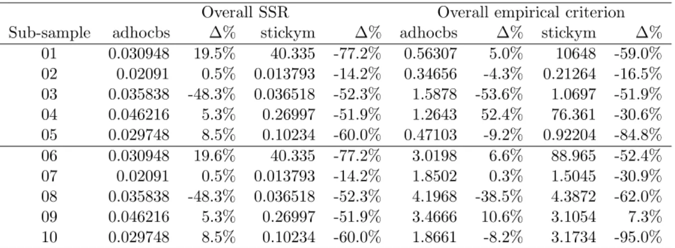
Table 5 summarizes the appropriateness of fit results over the whole 10 sub-samples. [Table 5 about here.]
The treefgd model has the lowest overall averaged SSR and empirical criterion among the methods under consideration. The ad hoc BS model has between 84 percent and 365 percent more overall SSR and 4 percent and 1200 percent more overall EC compared to treefgd. The out-of-sample performance of stickym and pca is even poorer. This result highlights the fact that reducing the dynamics of the whole IVS to only a small number of components, building a forecasting tool for such components, and then back-transforming to produce predictions of
the whole IVS, should be avoided, because some important information seems to go astray. For adhocbs and stickym, overall SSR does not depend on the size of the training data by construction, but overall empirical criterion values vary because the grid has changed. A training sample of only 60 days increases the overall averaged SSR for treefgd up to 100 percent. Thus, having enough information in the training sample is crucial to produce reliable predictions.
IV predictions with the sticky moneyness model and the ad hoc BS model depend only on the location parameter (m, τ) and on observed data in the past, as opposed to our model, which relies on a third location parameter (cp flag), several tuning parameters, exogenous factors and their predictions. It is much more complex, has a higher degree of freedom and is more difficult to fit than the models mentioned above.
Let us now examine as an illustrative example, 25 January 1999, the 15th OS day of the second sub-sample from 6 January 1998 to 31 December 1998. There are 242 calls and 218 puts in our database for that day. The IV for these options is estimated by the updated sticky moneyness model and updated ad hoc BS model, that is the models are fitted to the observed data of the day before, and not to the last day in the in-sample period of the sub-sample. Figures 9 and 10 show the results for call and put options separately.
[Figure 9 about here.] [Figure 10 about here.]
Although our model is not updated, it nevertheless produces predictions with reasonably small relative errors. The first 46 call and 38 put options with a time to maturity ofτ = 36526 are better estimated with our method 15 days out-of-sample than with the updated models and their one day out-of-sample estimate. This result supports the demonstrated high-predictive power of our model.
While comparing the middle- and long-term forecasting accuracy of updated models with our approach is unfair and inappropriate, adding cp flag as a third location parameter to stickym and adhocbs is a straightforward extension of these models. Based on either call or put options at the reference day, stickym and adhocbs are calculated separately for each type.
[Table 6 about here.]
As we shown in Table 6, the overall SSR of the three location parameter stickym model diminishes on all sub-samples (up to 77.2 percent!). Nevertheless, it is at least 193 percent higher than the overall SSR of treefgd. The out-of-sample forecasts still appear unstable. The introduction of the third location parameter in the adhocbs model can even increase its overall SSR.
5
Conclusions
We proposed a new methodology to estimate and, in particular, predict implied volatility surfaces. Our model is based on a semi-parametric additive expansion of simple fitted functions
using regression trees for the dynamics of implied volatilities. The proposed model can also be easily estimated in very high dimensions using a modified version of classical boosting procedures. Consequently, there is no need for variance reduction or other excluding data techniques to fit the model to real data, avoiding the possibility of a dangerous information loss.
We tested the predictive potential of our model on a huge data set of S&P 500 options collecting strong empirical evidence that our method performs reasonably well in forecasting short- and middle-term future implied volatilities (up to 60 days), and also under possible structural breaks in the time series. Moreover, our model outperforms different alternative approaches introduced in the literature if the final goal is implied volatility surface prediction.
A
Appendix: Functional gradient descent method
Gradient descent methods are an iterative way for finding a minimum of a functionf of several real-valued variables. The negative gradient gi = −∇f(Pi) is the direction of the steepest
descent at the pointPi. In the line search step, we findλi ∈R, such that Pi+1=Pi+λigi is
the lowest point along this path. Iterating those two steps leads to a sequence of points which converges to the minimum of f. The drawback of this method is that it converges slowly for functions which have a long, narrow valley. A better choice for the direction would be in this case the conjugate gradient.
Applying the steepest descent method in a function space F = {f | f : Rd −→ R}
leads, as the name indicates, to the FGD technique. Based on data (Yi, Xi), i = 1, ..., n, an
estimation of a function F ∈ F which minimizes an expected loss function E[λ(Y, F(X))], whereλ:R×R−→R+ is developed.
The FGD estimate of F(·) is found by minimizing Λ, the empirical risk, defined as: Λ(F)(x1, ..., xn, y1, ..., yn) = 1 n n X i=1 λ(yi, F(xi)). (13)
Starting from an initial function ˆF, the steepest descent direction would be given by the negative functional derivative −dΛ( ˆF). Due to smoothness and regularization constraints on the minimizer of Λ( ˆF), we must restrict the search to finding a function ˆf which is in the linear span of a class of simple base learnersSand close to−dΛ( ˆF) in the sense of a functional metric. This is equivalent to fit the base learner h(x, θ)∈ S to the negative gradient vectors:
Ui =− ∂λ(Yi, Z) ∂Z Z = ˆF(Xi) , i= 1, ..., n (14)
The minimal function F ∈ F is approximated in an additive way with simple functions ˆ fm(·) =h(·,θˆU,X)∈ S: ˆ FM(·) = M X m=0 ˆ wmfˆm(·), (15)
where the ˆwms are obtained in a line search step as in the previous procedure.
FGD is a derivative of boosting and bagging (cf. Friedman et al., 2000; Friedman, 2001). Audrino and B¨uhlmann (2003) already successfully apply FGD to estimate volatility in high-dimensional GARCH models, and Audrino et al. (2005) used it to model interest rates.
Some nonsymmetric loss functions are described in Granger (1999) and could be easily adapted to work in this framework. One of those loss functions is the LINEX function, which weights positive errors differently to negative errors. Most investors would agree on treating gains and losses differently. So for a >0:
LINEX = 1 N N X i=1 [exp{−a(ˆσIV i −σ IV i )}+a(ˆσ IV i −σ IV i )−1]
Acknowledgements
Financial support from the Foundation for Research and Development of the University of Lugano is gratefully acknowledged.
Notes
1The classification and regression tree (CART) algorithm was popularized by Breiman et
al. (1984). It is a set of logical if/then conditions for predicting or classifying.
2For a short introduction to FGD see the Appendix.
3ITM options have an intrinsic value. Therefore they cost more and there is less leverage
for speculation. The costs in portfolio hedging is higher with those options, hence they are traded less frequently.
4IV can be seen as predictor of future volatility.
5For simplicity, we modeled the log returns of each factor time series as an
ARMA(1,1)-GARCH(1,1) and used its mean forecast as predictor variable in the regression trees. Boot-strapping methods (such as filtered historical simulation) may reduce the forecast errors.
6Publicly available on the St. Lous Fed Homepage in the FRED data base.
7Other exogenous factors thought to be relevant for prediction can be easily taken into
References
Audrino, F., B¨uhlmann, P. (2003). “Volatility Estimation with Functional Gradient Descent for Very High-Dimensional Financial Time Series”, Journal of Computa-tional Finance 6, 1-26.
Audrino, F., Barone-Adesi, G., and Mira, A. (2005). “The Stability of Factor Models of Interest Rates”, Journal of Financial Econometrics 3, 422-441.
Bollen, N., and Whaley, R. E. (2004). “Does net buying pressure affect the shape of implied volatility functions?”, Journal of Finance, Vol. LIX, No. 2, 711-753. Breiman, L., Friedman, J.H., Olshen, R.A. and Stone, C.J. (1984). “Classification
and Regression Trees”, Wadsworth, Belmont (CA).
Cassese, G. and Guidolin, M. (2005). “Modelling the MIB30 Implied Volatility Sur-face. Does Market Efficiency Matter?”, Working Paper 2005-008A, Federal Reserve Bank of St. Louis.
Cont, R. and da Fonseca, J. (2002). “Dynamics of implied volatility surfaces”, Quan-titative Finance 2, 45-60.
Dumas, B., Fleming, J., and Whaley, R.E. (1998). “Implied Volatility Functions: Empirical Tests”, Journal of Finance, Vol. LIII, 6, 2059-2106.
Dupire, B. (1994). “Pricing with a smile”,RISK,7(1), 18-20.
Fengler, M. (2005).“Semiparametric Modeling of Implied Volatility”, Springer, Berlin. Fengler, M., H¨ardle, W., and Mammen, E. (2007). “A Semiparametric Factor Model for Implied Volatility Surface Dynamics”,Journal of Financial Econometrics, Vol. 5, No. 2, 189-218.
Friedman, J.H., Hastie, T., and Tibshirani, R. (2000). “Additive Logistic Regression: A Statistical View of Boosting”, Annals of Statistics 28, 337-407.
Friedman, J.H. (2001). “Greedy Function Approximation: A Gradient Boosting Ma-chine”, Annals of Statistics 29, 1189-1232.
Garcia, R., Luger, R., and Renault, E. (2003). “Pricing and Hedging Options with Implied Asset Prices and Volatilities”, Working Paper, CIRANO, CIREQ and Universit´e de Montr´eal.
Gon¸calves, S. and Guidolin, M. (2005). “Predictable Dynamics in the S&P 500 Index Options Implied Volatility Surface”, Working Paper 2005-010A, Federal Reserve Bank of St. Louis.
Granger, C.W.J. (1999). “Empirical Modeling in Economics: Specification and Eval-uation”, Cambridge University Press.
Gouri´eroux, C., Monfort, A., and Tenreiro, C. (1994). “Nonparametric diagnostics for structural models”, Document de travail 9405, CREST, Paris.
Gouri´eroux, C., Monfort, A., and Tenreiro, C. (1995). “Kernel M-estimators and functional residual plots”, Document de travail 9546, CREST, Paris.
Hentschel, L. (2003). “Errors in Implied Volatility Estimation”,Journal of Financial and Quantitative Analysis, Vol. 38, Issue 4, 779-810.
Heston, S.L., and Nandi, S. (2000). “A closed-form GARCH option valuation model”,
Review of Financial Studies, Vol. 13, Issue 3, Fall 2000, 585-625.
Poon, S.H., and Granger, C.W.J. (2003). “Forecasting volatility in financial markets: A review”, Journal of Economic Literature, 41, 478-539.
Implied volatilies of options on the S&P 500 index
Year 1996 1997 1998 1999
from 4 Jan 2 Jan 2 Jan 4 Jan
to 31 Dec 31 Dec 31 Dec 31 Dec
# Days 252 253 252 252 # Obs 69,705 100,554 106,571 116,207 Calls 35,090 49,986 56,522 62,187 ITM(m <1) 21,731 31,801 34,176 36,915 ATM (m= 1) 4 0 0 1 OTM(m >1) 13,355 18,185 22,346 25,271 Puts 34,615 50,568 50,049 54,020 ITM(m >1) 7,755 12,574 12,475 13,863 ATM (m= 1) 4 0 0 1 OTM(m <1) 26,856 37,994 37,574 40,156 Year 2000 2001 2002 2003
from 3 Jan 2 Jan 2 Jan 2 Jan
to 29 Dec 31 Dec 31 Dec 29 Aug
# Days 252 248 252 167 # Obs 107,325 98,281 107,730 71,514 Calls 62,265 59,586 62,087 36,870 ITM(m <1) 29,921 23,071 21,387 14,707 ATM (m= 1) 0 0 0 0 OTM(m >1) 32,344 36,515 40,700 22,163 Puts 45,060 38,695 45,643 34,644 ITM(m >1) 12,398 13,921 21,748 15,442 ATM (m= 1) 0 0 0 0 OTM(m <1) 32,662 24,774 23,895 19,202
Table 1: Implied volatilies of options on the S&P 500 index, total 777,887 observations on 1,928 days.
Descriptive statistics of the options’ data
1996 min Q1 mean median Q3 max std
m 0.5063 0.8751 0.9334 0.9526 1.0131 1.2367 0.1123
τ 0.0082 0.1205 0.4652 0.2575 0.6630 1.9699 0.4783
τ days 3 44 ≈170 94 242 719 ≈175
σIV, obs 0.0400 0.1400 0.1932 0.1700 0.2100 4.4400 0.1023
1997 min Q1 mean median Q3 max std
m 0.4066 0.8426 0.9199 0.9436 1.0162 1.4234 0.1382
τ 0.0082 0.1205 0.4912 0.2822 0.7315 1.9671 0.4918
τ days 3 44 ≈179 103 267 718 ≈180
σIV, obs 0.0700 0.1900 0.2540 0.2200 0.2600 4.9100 0.1585
1998 min Q1 mean median Q3 max std
m 0.3366 0.8236 0.9229 0.9414 1.0273 1.5669 0.1719
τ 0.0082 0.1205 0.5297 0.3288 0.8274 1.9644 0.5125
τ days 3 44 ≈193 120 302 717 ≈187
σIV, obs 0.0900 0.2100 0.3045 0.2600 0.3400 4.9000 0.1903
1999 min Q1 mean median Q3 max std
m 0.2861 0.8091 0.9177 0.9440 1.0297 1.4430 0.1743
τ 0.0082 0.1397 0.5668 0.4082 0.8740 2.2356 0.5141
τ days 3 51 ≈207 149 319 816 ≈188
σIV, obs 0.0400 0.2300 0.3032 0.2700 0.3400 4.9900 0.1642
2000 min Q1 mean median Q3 max std
m 0.3273 0.8451 0.9557 0.9706 1.0579 1.5774 0.1808
τ 0.0082 0.1288 0.5613 0.3781 0.8767 1.9699 0.5198
τ days 3 47 ≈205 138 320 719 ≈190
σIV, obs 0.0500 0.2000 0.2732 0.2400 0.2900 4.9200 0.1738
2001 min Q1 mean median Q3 max std
m 0.5460 0.8836 1.0279 1.0059 1.1357 2.0656 0.2110
τ 0.0082 0.1205 0.5166 0.3288 0.8110 1.9699 0.4954
τ days 3 44 ≈189 120 296 719 ≈181
σIV, obs 0.1000 0.2000 0.2786 0.2300 0.2900 4.8700 0.2001
2002 min Q1 mean median Q3 max std
m 0.5194 0.9017 1.0698 1.0371 1.2007 2.4461 0.2493
τ 0.0082 0.1288 0.5481 0.3589 0.8548 2.0082 0.5126
τ days 3 47 ≈200 131 312 733 ≈187
σIV, obs 0.0900 0.2000 0.2884 0.2400 0.3100 4.9500 0.2021
2003 min Q1 mean median Q3 max std
m 0.3954 0.8808 1.0432 1.0105 1.1787 2.1231 0.2493
τ 0.0082 0.1370 0.5833 0.3945 0.8932 1.9863 0.5427
τ days 3 50 ≈213 144 326 725 ≈198
σIV, obs 0.0800 0.1900 0.2693 0.2300 0.2900 4.7400 0.1813
Sub-samples description
Sub-sample Training data length CV ˆM Forecasting length Special day Special day In-sample period Out-of-sample period of interest of OS period 01 21 Jul 1997 - 16 Jul 1998 250 65 17 Jul 1998 - 09 Oct 1998 60 07 Aug 1998 16 02 06 Jan 1998 - 31 Dec 1998 250 106 04 Jan 1999 - 30 Mar 1999 60 07 Jan 1999 4 03 20 Dec 1999 - 13 Dec 2000 250 111 14 Dec 2000 - 13 Mar 2001 60 22 Jan 2001 25 04 15 Aug 2000 - 10 Aug 2001 250 32 13 Aug 2001 - 09 Nov 2001 60 17 Sep 2001 21 05 18 Mar 2002 - 13 Mar 2003 250 149 14 Mar 2003 - 09 Jun 2003 60 20 Mar 2003 5 06 22 Apr 1998 - 16 Jul 1998 60 21 17 Jul 1998 - 09 Oct 1998 60 07 Aug 1998 16 07 07 Oct 1998 - 31 Dec 1998 60 93 04 Jan 1999 - 30 Mar 1999 60 07 Jan 1999 4 08 20 Sep 2000 - 13 Dec 2000 60 74 14 Dec 2000 - 13 Mar 2001 60 22 Jan 2001 25 09 17 May 2001 - 10 Aug 2001 60 144 13 Aug 2001 - 09 Nov 2001 60 17 Sep 2001 21 10 16 Dec 2002 - 13 Mar 2003 60 125 14 Mar 2003 - 09 Jun 2003 60 20 Mar 2003 5 Table 3: In-sample (IS) and out-of-sample (OS) periods, as well as the special days of interest in the OS periods for the 10 different sub-samples under investigation. The optimal number ˆM of additive expansions is determined using cross-validation (CV) on the training data.
Specifications of the Heston-Nandi-GARCH (HNG) factors
HNG01 HNG02 HNG03 HNG04 HNG05 HNG06
m 0.8 1 1.2 0.8 1 1.2
τ 30 days 30 days 30 days 60 days 60 days 60 days
cp flag call call call call call call
HNG07 HNG08 HNG09 HNG10 HNG11 HNG12
m 0.8 1 1.2 0.8 1 1.2
τ 90 days 90 days 90 days 30 days 30 days 30 days
cp flag call call call put put put
HNG13 HNG14 HNG15 HNG16 HNG17 HNG18
m 0.8 1 1.2 0.8 1 1.2
τ 60 days 60 days 60 days 90 days 90 days 90 days
cp flag put put put put put put
Table 4: A time series of option prices for each constant option specification in the table is calculated via closed form solution in Heston and Nandi (2000). A rolling window of 500 days is used to fit the HNG model. It is shifted 30 days each time.
Appropriateness of fit
Overall SSR Overall empirical criterion Sub-sample treefgd adhocbs stickym pca treefgd adhocbs stickym pca
01 0.0141 0.025866 176.6954 0.034 0.51558 0.5363 25’968 0.68368 02 0.003167 0.020815 0.016084 0.056333 0.086613 0.36229 0.25465 0.88018 03 0.002873 0.069266 0.076482 0.064178 0.084765 3.4252 2.2222 1.458 04 0.010997 0.043908 0.5618 0.068075 0.26546 0.82934 110 1.4734 05 0.004024 0.027414 0.25583 0.101 0.14126 0.51867 6.0585 1.926 06 0.01537 0.025866 176.6954 0.049999 1.9137 2.8329 187.05 4.8194 07 0.004697 0.020815 0.016084 0.06723 0.48571 1.844 2.1758 8.6047 08 0.005764 0.069266 0.076482 0.050179 0.52494 6.8237 11.54 7.8384 09 0.013685 0.043908 0.5618 0.061624 0.93381 3.133 2.8952 6.6366 10 0.005902 0.027414 0.25583 0.083678 0.54276 2.0336 63.741 9.5796
Table 5: Overall SSR and empirical criterion (6) for the 10 sub-samples under investigation (see Table 3). The competing approaches are our new methodology based on tree-boosting (treefgd), an ad hoc Black and Scholes model (adhocbs), the sticky moneyness approach (stickym), and a principal components decomposition based model (pca).
Appropriateness of fit of three location models
Overall SSR Overall empirical criterion Sub-sample adhocbs ∆% stickym ∆% adhocbs ∆% stickym ∆%
01 0.030948 19.5% 40.335 -77.2% 0.56307 5.0% 10648 -59.0% 02 0.02091 0.5% 0.013793 -14.2% 0.34656 -4.3% 0.21264 -16.5% 03 0.035838 -48.3% 0.036518 -52.3% 1.5878 -53.6% 1.0697 -51.9% 04 0.046216 5.3% 0.26997 -51.9% 1.2643 52.4% 76.361 -30.6% 05 0.029748 8.5% 0.10234 -60.0% 0.47103 -9.2% 0.92204 -84.8% 06 0.030948 19.6% 40.335 -77.2% 3.0198 6.6% 88.965 -52.4% 07 0.02091 0.5% 0.013793 -14.2% 1.8502 0.3% 1.5045 -30.9% 08 0.035838 -48.3% 0.036518 -52.3% 4.1968 -38.5% 4.3872 -62.0% 09 0.046216 5.3% 0.26997 -51.9% 3.4666 10.6% 3.1054 7.3% 10 0.029748 8.5% 0.10234 -60.0% 1.8661 -8.2% 3.1734 -95.0%
Table 6: Overall SSR and empirical criterion (6) for the 10 sub-samples under investigation (see Table 3). The ad hoc Black and Scholes model (adhocbs) and the sticky moneyness approach (stickym) now depend on the three location parameters (m, τ,cp flag). The ∆% columns show their performances with respect to the same model with only two location parameters (m, τ).
0 0.2 0.4 0.6 0.8 1 1.2 1.4 0 0.2 0.4 0.6 0.8 1 1.2 1.4 1.6 0 0.2 0.4 0.6 0.8 1 1.2 1.4 Time to maturity τ 19 May 1998 Moneyness m
Weight with respect to selected grid point
Calls Puts Grid points Selected grid point
Figure 1: Illustrative example of weighting function. Weights with respect to a selected grid point, calculated with the weighting function (7) for 19 May 1998
0 1 2 3 4 5 0 0.1 0.2 0.3 0.4 0.5 0.6 0.7 0.8 0.9 1 ω1(m) = 1 / π * arctan( α 1 (m−1)) + 1/2, for a call = 1 / π * arctan( α 1 (1−m)) + 1/2, for a put call put 0 1 2 3 4 5 0.1 0.2 0.3 0.4 0.5 0.6 0.7 0.8 ω2(τ) = 1 / π * arctan( α 2 (1−τ)) + 1/2
Figure 2: Illustrative example of weighting function on 18 May 1998. Plots of the w1(m)
Jan96 Jan97 Jan98 Jan99 Jan00 Jan01 Jan02 Jan03 Jan04 400 600 800 1000 1200 1400 1600
S & P 500 daily close prices
Jan96 Jan97 Jan98 Jan99 Jan00 Jan01 Jan02 Jan03 Jan04 −0.08 −0.06 −0.04 −0.02 0 0.02 0.04 0.06
S & P 500 daily log returns
Figure 3: Close and log return of the S&P 500. The circles mark the following dates: 7 August 1998 (bomb attacks on US embassies in Africa), 7 January 1999 (opening of impeachment trial against President Clinton), 7 November 2000 (presidential election), 22 January 2001 (1st day after President Bush’s oath of office), 17 September 2001 (few days after the 11 September terrorist attacks), 20 March 2003 (invasion of Iraq)
20−Apr−19980 09−Aug−1998 28−Nov−1998 19−Mar−1999 0.5 1 1.5 2 2.5 3 3.5 4 4.5 5 5.5
Call option, issued 20−Apr−1998 Strike K = 700, expiry date T = 20−Mar−1999
IV
Figure 5: Initial model F0(m, τ,cp flag,factors) fitted on 20 December 1999 to 13 December
2000. In theupper panel,Fc
0(m, τ,factors) has been fitted as regression tree with 10 leaves. In
thelower panel, the same forF0p(m, τ,factors). No other variables thanm andτ were chosen by the regression tree algorithm. Note that superscriptsc and p indicate that the tree is fit for call and put options separately.
Figure 6: This figure shows the 21st step of ˆM = 111 in an additive expansion of regression trees with five leaves. tree[c(m, τ,factors) in the upper panel, tree[p(m, τ,factors) in the lower
panel. Past and future values of Heston Nandi GARCH (HNG) factors have been chosen by the regression algorithm for treec. The data ranges from 20 December 1999 to 13 December
2000. Note that superscripts c and p indicate that the tree is fit for call and put options separately.
0 10 20 30 40 50 60 0 0.05 0.1 0.15 0.2 0.25 Daily average of SSR Out−of−sample day t Daily SSR t treefgd adhocbs stickym pca 7 Aug 1998 0 10 20 30 40 50 60 −50 0 50 100 150 200 250 300 350 400 450 500
SSR relative to our model
Out−of−sample day t Difference in % 0 10 20 30 40 50 60 0 0.5 1 1.5 2 2.5 3
Daily average of loss
Out−of−sample day t
Daily EC
t
Figure 7: OS performance results on sub-sample 1. Upper panel: Daily averaged SSRt as in
(11). Central panel: Daily averaged gains/losses with respect to our treefgd model. Lower
panel: Daily averaged empirical criterion (6). Performance measures are reported for the four competing approaches introduced in the paper: our model (treefgd), an ad hoc Black and Scholes model (adhocbs), the sticky moneyness approach (stickym), and a principal
compo-0 10 20 30 40 50 60 0 0.05 0.1 0.15 0.2 0.25 Daily average of SSR Out−of−sample day t Daily SSR t treefgd adhocbs stickym pca 17 Sep 2001 0 10 20 30 40 50 60 −100 0 100 200 300 400 500
SSR relative to our model
Out−of−sample day t Difference in % 0 10 20 30 40 50 60 0 0.5 1 1.5 2 2.5 3
Daily average of loss
Out−of−sample day t
Daily EC
t
Figure 8: OS performance results on sub-sample 4. Upper panel: Daily averaged SSRt as in
(11). Central panel: Daily averaged gains/losses with respect to our treefgd model. Lower
panel: Daily averaged empirical criterion (6). Performance measures are reported for the four competing approaches introduced in the paper: our model (treefgd), an ad hoc Black and Scholes model (adhocbs), the sticky moneyness approach (stickym), and a principal
compo-0 50 100 150 200 250 0 0.5 1 1.5 2 2.5 Call option nr. IV treefgd observed 0 50 100 150 200 250 −1 −0.5 0 0.5
Relative error: (treefgd−observed)/observed
Call option nr. Relative error 0 50 100 150 200 250 0 0.5 1 1.5 2 2.5 Call option nr. IV stickym updated observed 0 50 100 150 200 250 −1 −0.5 0 0.5
Relative error: (stickym updated−observed)/observed
Call option nr. Relative error 0 50 100 150 200 250 0 0.5 1 1.5 2 2.5 Call option nr. IV adhocbs updated observed 0 50 100 150 200 250 −1 −0.5 0 0.5
Relative error: (adhocbs updated−observed)/observed
Call option nr.
Relative error
Figure 9: Comparing 15thOS day predictions of our model with the ones of the updated sticky moneyness and of the updated ad-hoc BS model. 242 observed IVs from call options on 25 January 1999 are plotted in a row. Increasing τs from left to right.
0 50 100 150 200 250 0 0.5 1 1.5 2 Put option nr. IV treefgd observed 0 50 100 150 200 250 −1 −0.5 0 0.5
Relative error: (treefgd−observed)/observed
Put option nr. Relative error 0 50 100 150 200 250 0 0.5 1 1.5 2 Put option nr. IV stickym updated observed 0 50 100 150 200 250 −1 −0.5 0 0.5
Relative error: (stickym updated−observed)/observed
Put option nr. Relative error 0 50 100 150 200 250 0 0.5 1 1.5 2 Put option nr. IV adhocbs updated observed 0 50 100 150 200 250 −1 −0.5 0 0.5
Relative error: (adhocbs updated−observed)/observed
Put option nr.
Relative error
Figure 10: Comparing 15th OS day predictions of our model with the ones of the updated sticky moneyness and of the updated ad-hoc BS model. 218 observed IVs from put options on 25 January 1999 are plotted in a row. Increasing τs from left to right.