Determinants of Capital Structure in Listed Norwegian Firms

(1)

NHH – Norges Handelshøyskole

and

Lancaster University

Bergen/ Lancaster, Fall 2014

Determinants of Capital Structure in Listed

Norwegian Firms

Cathrine Marie Nilssen

Supervisors: Floris Zoutman (NHH) & Robert Read (Lancaster University)

Master’s Thesis, Double Degree (NHH & Lancaster University)

This thesis was written as a part of the Double Degree programme between NHH MSc in Economics and Business Administration, Major Financial Economics, and Lancaster University Management School MSc in International Business. Neither the institutions, the supervisor(s), nor the censors are - through the approval of this thesis -

responsible for neither the theories and methods used, nor results and conclusions drawn in this work.

(2)

Abstract

The main goal for most firms is to maximise firm value and the wealth of shareholders. In order to achieve this goal, firms should use an optimal combination of equity and debt that will result in a low weighted average cost of capital for the firm. It is therefore necessary for firms to be aware of the factors that influence their capital structure decision.

Several empirical studies have attempted to explain what determines the choice of capital structure in firms. However few have focused solely on Norwegian firms. Hence, the primary objective of this study is to examine what determines the capital structure in listed Norwegian firms.

DataStream was used to obtain the data needed for the statistical analysis and previous studies were used to calculate the measures for the firm-specific characteristics. The study was conducted over a period of 7 years, from 2007 to 2013, and there were a total of 90 firms in the sample, resulting in 876 observations.

The results from the study indicate that tangibility is the most important firm

characteristic to consider when making capital structure decisions. Furthermore, the results indicate a difference between the book value and market value of debt. Book value of leverage finds support in the pecking order theory, while none of the theories fully explains the observed capital structure in Norwegian firms. Based on the evidence obtained from this research, firms should take these firm-specific factors into account when making capital structure decisions.

(3)

Acknowledgements

I would like to express my gratitude to the people in my life that has shown their support throughout my entire learning, research and writing process.

To all the lecturers and classmates from NHH and Lancaster University that has made my years as a master’s student into an unforgettable experience.

Although words will never be enough, I want to thank my parents and my brothers for always being there for me. Their support, care and love is what got me here today. I never could have done it without them.

(4)

Chapter 1: Introduction

The first chapter in this paper will give an introduction to the topic of capital structure and an overview of the thesis. This chapter will consist of four sections, background to the research topic, purpose of study, aims and objectives and an outline of the structure. 1.1Background

Modern theory of capital structure began with Miller and Modigliani (1958) and their famous proposition that described how and why capital structure is irrelevant. Since then, an extensive amount of research has focused on how companies decide between equity and debt for financing. The financial crisis of 2008 contributed to increased attention towards capital structure decisions, as it highlighted the importance of deviations from Miller and Modigliani’s irrelevance theorem (Kashyap and Zingales, 2010).

Several researchers have tried to determine what factors affect companies’ financing decision. Overall this has resulted in two main theories, the pecking order theory and the trade-off theory. The trade-off theory explains that the choice of capital structure is a result of a trade-off between the benefits of debt, such as the debt tax shield, and the costs of debt, including bankruptcy costs and costs of financial distress. By contrast, the pecking order theory advances that companies prefer the cheapest source of funding. Because of information asymmetry, companies will prefer internal to external funding and debt over equity (Myers, 1984).

The two theories of capital structure represents the basis for many studies that have been done later, in which the analysis try to determine which model best explains the choice of financing and what factors might make up the capital structure decision.

(8)

However past empirical research has provided contradictory results and evidence of the theories’ ability to explain capital structure remains limited. Researchers

continuously strive to determine the most important determinants of capital structure and how it varies across companies, industries and countries.

This thesis analyses the explanatory power of established theories and firm-specific factors from the literature in explaining the choice of capital structure across

Norwegian listed firms. This study is based on a panel data set from 2007 to 2013 and consists of 90 companies listed on the Oslo Stock Exchange. This study will use panel data regression analysis to empirically understand how different firm-specific factors impact firms’ leverage ratio.

1.2 Research problem

The combination of debt and equity for a firm represents a firm’s target capital structure, and is one of the most important decisions a firm has to make. In order to determine the target, firms should be aware of the factors that can influence their choice of capital. Based on previous empirical research, six firm-specific characteristics were chosen for this study; profitability, size, growth, tangibility, liquidity and non-debt tax shield. Furthermore, the effect of these characteristics will be examined for two measurements of leverage, book value and market value.

Several studies on this topic have already been conducted for different countries. However, except for Frydenberg (2004) and his research on capital structure in the Norwegian manufacturing sector, few have focused solely on the determinants of capital structure for Norwegian firms. This represents a gap in the existing literature and provides a purpose for this study.

(9)

1.3 Aims and Objectives

The aim of this study is to determine the effect firm-specific characteristics have on the capital structure of Norwegian listed firms. Based on this, the following secondary objectives have been formulated:

 Analyse whether firm-specific characteristics can explain the variation in capital structure across Norwegian firms.

 Determine if book value of leverage and market value of leverage produce different results.

 Look at the dominant theories of capital structure and examine if the trade-off theory and the pecking order theory can explain the observed capital structure of Norwegian firms.

1.4 Outline

Following the introduction, this paper is structured into four chapters 1. Introduction

The first chapter describes the background for this paper, followed by the purpose of study and a presentation of the aims and objectives of this thesis. 2. Theoretical Framework:

This chapter will present capital markets in a perfect and an imperfect setting, discuss the propositions of Miller and Modigliani and present the two most dominant theories of capital structure, the pecking order theory and the trade-off theory. Furthermore, previous empirical research will be analysed and discussed and an overview of how Norwegian companies have access to capital

(10)

will be presented. Finally, the determinants of capital structure used in this paper will be presented.

3. Methodology:

This chapter will present hypotheses that will be tested in this paper, as well as the research methods used. How the data is collected will also be described and estimation methods will be evaluated and illustrated.

4. Analysis:

The fourth chapter will analyse the data by using the most feasible estimation model found in the previous chapter. The hypotheses will be tested and based on this the findings will be presented.

5. Conclusion:

This chapter will summarise this research paper and provide a conclusion, present the limitations of the study and provide recommendations for future research

(11)

Chapter 2: Theoretical framework

This chapter will first explain capital structure in a perfect market and present Miller and Modigliani proposition I and II. Thereafter, capital structure in an imperfect market will be explained by using the two main theories of capital structure; the trade off theory and the pecking order theory. Then I will discuss imperfect capital markets, before previous empirical research on the determinants of capital structure will be evaluated. This section will also include cross-country studies that involve Norway.

2.1 Defining capital Structure

The overall purpose of a firm is to maximise firm value and create value for

shareholders. Firm value is calculated by the present value of its expected future cash flows, discounted by the weighted average cost of capital. In order to maximise the value of the firm, management need to make investments in order to generate cash flows. These investments requires funds and companies have to decide whether they want to use debt or equity. The optimal mix of debt and equity can minimise the weighted average cost of capital and increase shareholder value, and consequently the value of the firm (Berk and DeMarzo, 2013). Capital Structure is an expression of how a company is financing its total assets and is a decision that poses a lot of challenges for firms. Determining an appropriate mix of equity and debt is one of the most strategic decisions companies are confronted with (Modugu, 2013, p. 14). A firm has three main sources of financing at their disposal to fund their investments. This includes the use of retained earnings, issuing new shares and borrowing money. Together these financing options represent a firm’s capital structure, as well as its ownership structure.

In 1958 Miller and Modigliani stated that capital structure was irrelevant as the value of the company would be the same regardless of how a company is financed. Based on

(12)

this, discussions and theories have been developed in the literature aiming to explain if an optimal capital structure exists and what factors are determining the choice of capital structure. According to Myers (2003, p. 3) there does not exist a universal theory of capital structure, only useful conditional theories that differ in the factors that affect the choice of capital structure. The following chapter will present theories that are relevant for my research question and I will explain and discuss why I believe these theories are important for my analysis. Furthermore I will briefly present past studies on the determinants of capital structure.

2.2 Capital structure in a perfect market

With perfect capital markets there is not possible to influence a company’s value through how the company is financed. Capital markets are said to be perfect in the absence of agency costs, taxes, transaction costs and asymmetrical information. In the real world, capital markets are not perfect. However, it can be useful to evaluate how closely the assumptions hold and consider the consequences of any deviations (Berk & Demarzo, 2013).

2.2.1. Miller and Modigliani

“The pizza delivery man comes to Yogi Berra after the game and says, Yogi, how do you want this pizza cut, into quarters or eights? And Yogi says, cut it in eight pieces. I’m feeling hungry tonight” 1_{(Miller, 1997 explains the irrelevance theorem)}

(13)

The first important insights into the choice of capital structure and its correlation with firm value started with Miller and Modigliani in 1958. Under the conditions of perfect capital markets they demonstrated the following regarding the role of capital structure in determining firm value (Berk & Demarzo, 2013):

M&M proposition I: In a perfect capital market, a company’s total market value is independent of its capital structure

Formula 1: Miller & Modigliani Proposition I:

VL = VU = VA

The proposition implies that the total market value of a firm’s securities is equal to the market value of its assets, regardless of whether the firm is leveraged or not. The cost of debt has traditionally been lower then that of equity when calculating the capital requirements, as debt is less risky. Arguably it will therefore be more beneficial to finance a company with debt, as it is relatively cheaper. However Miller and Modigliani states that the capital composition of a company is irrelevant as it does not affect the company’s cash flow or its market value (Miller and Modigliani, 1958). On the balance sheet, the total market value of a firm’s assets equals the total market value of the firm’s liabilities, including securities issued to investors. Changing the capital structure will therefore only alter how the value of the assets is divided across securities, but not the total value of the firm (Berk and Demarzo, 2014). In a perfect capital market it would not be a problem for an investor to replicate any capital composition.

Their second proposition, which is a direct development of the first one, discusses how risk and return on equity change as a result of alterations in the debt ratio:

M&M proposition II:The expected return on equity in a leveraged company will increase proportionally with the debt-to-equity ratio.

(14)

By interpreting formula 1 in terms of market values we get the following expression:

Formula 2: Cost of unlevered equity (Pretax WACC)

By solving formula 2 for rE we get the following expression for the levered return on

equity (Berk and Demarzo, 2013):

Formula 3: Miller & Modigliani Proposition II

The return on levered equity (rE) equals the unlevered return (rU), plus and extra

“kick” because of leverage (D/E*(rU-rD)). This effect causes an even higher return on

levered equity when the firm performs well (rU > rD), but makes it drop even lower

when the firm performs poorly (rU < rD) (Berk and Demarzo, 2013).

Miller and Modigliani’s theory provides a theoretical framework for understanding capital structure. However, it does not provide a realistic description of how

companies should decide on an optimal capital structure (Frank & Goyal, 2005). By assuming perfect capital markets, they rather highlight the factors such as, taxes, asymmetry, bankruptcy etc. that makes capital structure relevant. As a result, their theory has been groundbreaking in the field of corporate finance and provides an important foundation for understanding capital structure.



r_u  E

EDre D EDrd

(15)

2.3 Capital structure in an imperfect market

In reality, capital markets are not perfect, and the assumptions that Miller and Modigliani made did not consider factors such as the tax advantages of debt, asymmetric information, bankruptcy costs and financial distress. However in 1963 they modified their propositions in order to account for the tax benefits of debt. Today there are two main theories trying to explain how companies allocate their capital in an imperfect market, the “Trade-off theory” and the “Pecking order theory” (Myers, 1984).

2.3.1 Taxes and Capital structure

Miller and Modigliani (1963) modified their propositions and considered the interest rate on debt to be offset by the tax savings from the interest tax shield. They assumed that debt was risk-free and would be held permanently, so that the value of the tax shield could be considered a perpetuity (Berk and DeMarzo, 2013):

PV (interest tax shield) =

Proposition I can now be rewritten as: VL = VU +

By including taxes in formula 2, we can an expression for the weighted average cost of capital.

Formula 4: The Weighted Average Cost of Capital

 _c(r_f D) r_f cD  _c D  r_wacc E EDrE D EDrD(1c)

(16)

The weighted average cost of capital represents the effective cost of capital to the firm, after including the benefits of the interest tax shield. The higher the firm’s leverage, the more the firm will exploit the tax advantages of debt, and the lower its WACC is. When making financing decisions, the capital used should be a weighted average of the various costs of each capital component. (Berk and DeMarzo, 2013)

2.3.2 The Static Trade-Off theory

The Trade-Off theory emerged as a result of the debate over the Miller & Modigliani theorem (Frank and Goyal, 2008). The theory states that the “…total value of a levered firm equals the value of the firm without leverage plus the present value of the tax savings from debt minus the present value of financial distress costs” (Berk and DeMarzo, 2013, p. 574).

Formula 5: VL = VU + PV (Interest Tax Shield) – PV (Financial Distress Costs)

Where VL_{is leveraged firm value, V}U_{is unleveraged firm value and PV is present value.}

The optimal level of debt is what maximizes VL_{. To maximise firm value, companies will}

operate at the top of the curve in figure 1.

(17)

According to Myers (1984), more debt involves increased costs associated with

bankruptcy and financial distress. When the risk of incurring these costs increases, the value of the firm will decrease and capital will become more expensive. As a result, there exists an optimal capital structure that reflects a trade-off between the costs of bankruptcy or financial distress and the tax benefits of debt. This implies that

companies should set a target financial debt ratio (Frank and Goyal, 2008; Swinnen et al., 2005). However the optimal debt ratio will vary across firms because tax rate, bankruptcy costs and the impact of financial distress vary across firms. With regards to determinants of capital structure, the theory claims that profitable firms will try to protect their profits from debt, resulting in a higher level of leverage. Furthermore, growth will have a negative impact on debt because the risk of financial distress will be higher for growing firms.

2.3.3 Pecking order theory

The Pecking order theory was developed by Stewart C. Myers in 1984 and defines a ranking of preferred capital. Furthermore Myers (2003, p. 3) claims that“…financing adapts to mitigate problems created by differences in information between insiders and outside investors”. The theory can be explained from the existence of transaction costs and the perspective of asymmetric information (Swinnen et al. 2005). Because of this, companies prefer retained earnings to debt and will only under extreme circumstances use equity as financing (Myers, 1984). As a result, variation in a company’s debt level is driven by the company’s net cash flow and not by the trade-off between the costs and benefits of debt (Fama & French, 2002). Information asymmetry occurs when the owner-managers have full information about the true value and quality of the company, whereas

(18)

investors have less information. This makes it difficult for investors to separate good and bad quality companies. Investors make up for this uncertainty by requiring a higher rate of return and thus make capital more expensive for companies (Frank & Goyal, 2008). Asymmetric information can in turn lead to adverse selection problem

Under pecking order conditions companies prefer internal to external financing. Therefore profitable firms will borrow less as they have more internal financing

available (Myers, 2003, p. 27) and less profitable firms will use more debt. There is no specific debt-to-value ratio for firms in this theory, so the level of debt a company has incurred reflects the need for external finance, rather than a specific target (Myers, 1984, p. 576). Furthermore, companies with more volatile net cash flows are according to the theory, are more likely to have less leverage (Fama & French, 2002)

Figure 2: Pecking order Theory

Source: Own contribution

1 Internal

Financing

Retained Earnings

2 External

Financing

Debt

3 External

Financing

Equity

(19)

2.3.4 International Capital Markets

International capital markets have experienced rapid changes since the mid 1970’s. Financial markets have been deregulated, capital controls have been reduced, new financial instruments have emerged and investors have seen the benefit of reduced risk in holding a diversified portfolio. In addition, new technology has led to lower transaction costs and made the access to international markets easier (Errunza & Miller, 2000). Despite this, research have shown that investors prefer to invest in their home country regardless of the lower risk associated with holding an international portfolio. This implies that it exist barriers to international capital mobility and thus capital markets are imperfect (Bayoumi, 1997). The literature presents several factors that may serve as barriers to international capital mobility. Medeiros & Quinteiro (2008) suggest that transaction costs is the main barrier, stressing that it will induce concentration in domestic portfolios. Transaction costs include taxes and restrictions to capital markets, as well as informational disadvantages. Additionally, Eiteman et al (2013) states that other barriers include exchange rate risk, illiquidity in the domestic financial market and different market risk-return trade offs.

2.3.4.1 The Cost of Capital

The capital market imperfects have important influence on a firms’ marginal cost of capital, and thus their weighted average cost of capital (See appendix A).

The availability of capital depends on whether a firm can gain liquidity for its securities and their price based on international rather than national standards. Eiteman et al. (2013, p. 382) stresses that firms that are able to attract foreign investors can

“…escape the constraints of their own illiquid or segmented market”. Furthermore the international availability of capital to firms may let them lower their cost of equity and

(20)

debt. In addition, it allows firms to maintain a desired debt ratio, even if significant amounts of debt need to be raised. Arguably, as a result, firm’s that have the

opportunity to source funds internationally have a constant marginal cost of capital for large parts of their capital budget (Eiteman, 2013). However empirical studies differ in their results regarding whether or not multinational firms have a higher cost of capital compared to firms that only source funds domestically.

Henderson et al. (2006) mentions several reasons for why firms would choose to raise capital in globally rather than in their home country, including risk sharing, lower cost of capital and potentially lower transaction costs. They find evidence of credit market segmentation and that a volatile environment affects capital structure choice for firms. Moreover, they argue that a firms’ decision to issue equity is influenced by both firm-specific factors and macroeconomic conditions. They show that firms are more likely to issue equity in favourable macroeconomic conditions where the equity market is overvalued. This research is supported by studies conducted by Stultz (1995), Singh & Nejadmalayeri and Errunza & Miller (2000) who also provide evidence of the beneficial impact of sourcing funds internationally in order to gain a lower cost of capital.

However Lee & Kwok (1988) arrived at the opposite conclusion when they discovered evidence that international funding could potentially lead to a higher cost of capital. Their study found that multinational firms have higher bankruptcy costs, political risk and asymmetric information compared to firms that kept to their domestic capital markets.

(21)

2.4 Empirical research

Previous empirical research regarding capital structure provides no general model on the determinants of capital structure. Appendix B.1 lists some recent studies on the matter and it shows that each researcher considers different factors when analysis the level of debt for companies. After considering the available data, the most common determinants based on previous research and theory was decided upon. As a result, the final set of independent variables includes six factors; Profitability, non-debt tax shield, tangibility, firm size, liquidity and growth.

2.4.1 Analysis of selected previous empirical research

Antoniou et al. (2002) researched the determinants of capital structure of French, British and German companies using panel data from 1969-2000. They chose to examine these countries together as they are characterised by different financial systems and traditions, something that may affect the amount of leverage in a company. Surprisingly enough, their findings suggest that factors affect the three countries in the same way despite of this. Further they get a positive relationship between leverage and size, while the opposite is the case for growth and leverage. For fixed assets, profitability and effective tax rates, they discover that the factors varies in the direction and degree of influence on leverage across the sample countries. This shows that capital structure decisions do not only depend on firm-specific factors, but also the environment the company operates in.

Nunkoo & Boateng (2009) researched non-financial Canadian companies between 1996 and 2004 using panel data and a dynamic regression model. Their result suggested that firms have long-term target debt ratios, but with a slow adjustment ratio. Furthermore they find that profitability and tangibility have a positive effect on

(22)

the amount of leverage a company has, while there was a negative effect based own size and growth opportunities.

Titman & Wessels (1988) researched the explanatory power of different factors from theories of optimal capital structure. Their data is collected from American industrial companies from 1974-1982. They did not find any significant relationship between leverage and volatility, tangibility, growth and non-debt tax shield. However, they discovered a negative relationship between debt and profitability and a negative correlation between size and short-term debt. The most surprising discovery in their study is that the level of debt is negatively correlated with the uniqueness of the company.

Frank & Goyal (2004) did a similar study but on publicly traded U.S firms from 1950 to 2000. They discover that firms tend to have lower levels of debt the more profitable they are. Furthermore their results suggest that firm tangibility is significant and causes firms to have more debt, the more collateral they have. In addition they conclude that larger firms tend to have more leverage compared to smaller firms. Finally they found that dividend-paying firms have less leverage and that leverage tends to be higher when the US inflation rate is high. Overall they find that the pecking order theory does a poor job in explaining capital structure.

Frydenberg (2004) has conducted one of the few empirical studies that have been done on capital structure of Norwegian firms. He focuses on firms in the Norwegian

manufacturing sector between 1990 and 2000. He discovers that the pecking order theory finds significant support in the results of the study. His findings suggest that profitable firms tend to have less debt and that firms with a large amount of fixed

(23)

non-debt tax shield is significant and negative in his study. Which indicates that firms substitute debt for such tax shields.

2.4.2 Cross-country studies including Norway

As presented in the previous section, there has been a lot of research conducted

regarding capital structure. However, few have focused solely on Norway, which leaves a gap in relation to knowledge concerning capital structure in Norwegian firms.

Nevertheless, some cross-country studies have included subsamples of Norwegian companies when exploring differences in capital structure across countries. Because country-specific factors, including institutional differences, may induce a change in the determinants of capital structure, this may help decide on what determinants are most important for Norwegian companies. It will also be of interest to explore potential differences in the results related to prior research.

Bancel and Mittoo (2004) surveyed managers in sixteen European countries on the determinants of capital structure. They discovered that financial flexibility is the most important factor when issuing debt, while earnings per share dilution is the primary concern when issuing common stock. In their survey, 91% of managers’ rank financial flexibility as important compared to only 59% of US CFO’s in a survey conducted by Graham and Harvey (2001). This difference may suggest that European companies would try to preserve financial flexibility by keeping a lower level of debt. Bancel and Mittoo (2004)’s results suggest that the differences in firms’ financial decisions across countries are the most significant between Scandinavian and Non-Scandinavian firms. La Porta et al. (1997) examined the ability of firms in different legal environments to raise external finance through equity or debt. They confirm that countries’ legal rules matters for the size of a country’s capital markets and that differences in shareholder

(24)

rights, bankruptcy law and the quality of law enforcement have strong impact on capital structure. Furthermore they find that the credit rates in Norway are stronger than in US, but shareholder rights are weaker. This implies that we should expect a higher debt level in Norway compared to the US.

Levine et al. (1999) states that Norway can be considered a country with a bank-based financial system. This suggests that most companies finance themselves through bank loans, in contrast to market based financial systems, like the US, where firms mostly fund themselves through the capital markets. It is often assumed that companies in bank-based countries have higher leverage and more short-term debt. His results however indicate that there is no cross-country empirical evidence for the superiority of either the bank-based or the market-based financial system. As a conclusion he suggest that specific laws and enforcement mechanisms that govern debt and equity transactions are more useful in describing cross-country capital structure.

2.4.3 Summary of previous empirical research

Overall the results from previous empirical research show that in general, the same characteristics affect the choice of capital structure across countries, however

institutional factors may lead to differences in the sensitivity of these factors. Previous empirical papers are reaching contradictory results in their investigation of the

relationship between capital structure and company specific factors. There are differences both across industries and geographic areas, as well as considerable variation within individual industries. Even though the effect of the capital structure determinants differs, there are still indications that the same factors are evident across several studies.

(25)

2.5 Firm-Specific Determinants of capital structure

There is a large amount of possible determinants of capital structure choice. This makes it challenging to decide which are the most important and how to establish a good model to measure the different variables and their degree of significance (Harris & Raviv, 1991). However, there is still some consensus amongst researchers that there exist some common factors. The two theories described in chapter 2, mostly agrees on the factors that determines how a company is finances. However, the assumptions and expectations on the extent and direction of how the factors affect capital structure differ between the theories.

This section will present a brief discussion on the determinants that different theories of capital structure suggest may affect the amount of leverage in firms. These

determinants are profitability, size, tangibility, growth, liquidity and non-debt tax shield. These determinants, their relationship to capital structure and their link to established theories will be discussed individually below.

Profitability

Profitability has been the most significant determinant in previous studies regarding capital structure. It indicates how well management are able to utilise total assets to generate earnings. According to the trade-off theory, the higher the profitability of the firm, the more likely the company is to issue debt as it is reducing its tax liability. In addition, firms with high a high profitability ratio have less risk of bankruptcy and financial distress. Moreover, debt providers will be more willing to lend to profitable firms because the probability of default is lower. Therefore the theory predicts a positive relationship between leverage and probability. In comparison, the pecking order theory predicts a negative relationship, as companies prefer to finance

(26)

themselves through retained earnings. A profitable firm will retain more earnings and as a result, the leverage needed should decrease. Nunkoo and Boateng (2009) studied the capital structure in Canadian firms and discovered a significant positive

relationship between profitability and debt. However most of the previous empirical research shows that profitability has a negative effect on leverage (Shah & Khan, 2007; Gonsález & Gonsáles, 2012; Ozkan, 2001; etc.).

Size

Size is also linked with the leverage of a company. According to the trade-off theory large firms will have less risk because they are more diversified and have more stable cash flow. Hence, larger firms will have a lower financial distress costs and a lower probability of bankruptcy costs. Additionally, larger firms will have a better reputation in the debt market because they would receive higher credit ratings since their default risk is lower. This implies a positive relationship between size and leverage (Frank & Goyal, 2005; Titman & Wessels, 1988). With regards to the pecking order theory, Rajan and Zingales (1995) suggested that this relationship could be negative. Larger firms have less information asymmetry. Consequently, the chance of issuing undervalued equity is reduced and will encourage larger firms to use equity financing. Frank and Goyal (2009) agrees, and argues that larger firms have easier access to the capital market than their smaller counterparts. As a result, it will be easier to attract equity and these firms will thus have less debt. Previous studies vary in concluding whether size is a significant factor for capital structure. Empirical studies done by Chen (2004), Mazur (2007), Nunkoo & Boateng (2009) amongst others, found a negative

(27)

discovered a positive relationship. Other studies found that size did not have any significant impact on leverage (Shah & Khan, 2007; Noulas & Genimakis, 2011, etc.). Tangibility

Tangible assets include fixed assets, such as machinery and buildings, and current assets, such as inventory. Compared to intangible, nonphysical assets, tangible assets are easier to collateralize so they will suffer a smaller loss if the company goes into financial distress. Tangible assets are associated with a higher leverage ratio as they can serve as better collateral for debt (Rajan & Zingales, 1995). Moreover, a high tangibility ratio will lower expected agency costs and problems. According to both theories, tangibility will positively affect leverage (Frank & Goyal, 2009). This is consistent with the majority of previous empirical research (Shah & Khan 2007; Chen, 2004; Nunkoo & Boateng 2009 etc.) that discovers that companies with more tangible assets has higher leverage ratios. However, Booth et al. (2001) suggests a negative relationship between tangibility and debt based on their results.

Growth

According to Frank & Goyal (2005; 2009), there should be a negative relationship between leverage and growth opportunities based on the trade-off theory. This is mainly because growing firms loose more of their value when they go into financial distress than mature firms. Growing firms will also have higher agency costs of debt because debt holders fear that these growing firms will invest in risky projects for the future (Booth et al. 2001). As a result, growth will reduce firm leverage. This is

consistent with the results from Olayinka (2011) and Ozkan (2010). By contrast, Chen (2004) and Booth et al. (2001) estimated a positive relationship between leverage and growth. According to the pecking order theory, growing firms should get more debt

(28)

over time if internal funds are not sufficient to finance investment opportunities. Hence the amount of leverage in growing firms should be considerably more than for a

stagnant firm. Liquidity

Liquidity can be defined as the ability for firms to use current assets to cover their current liabilities. Thus, it says something about how well firms meet their short-term obligations. In the pecking order theory, internal financing is the most preferable source of capital for firms. Therefore, companies are more likely to create reserves from retained earnings (Ali et al. 2013). Firms that are able to convert their assets into cash, use these inflows to finance their investments instead of using debt. Conclusively, liquidity will have a positive effect on leverage. This is supported by the research conducted by Sbeiti (2010) and Ozkan (2001).

Non-Debt Tax Shield

According to Ali et al. (2013) debt financing is less attractive if non-debt related corporate tax shields exist, such as investments or depreciation. Companies can use these non-interest items to reduce their tax bills. In other words, according to the trade-off theory, companies with higher non-debt tax shield are likely to use less debt (Titman & Wessels, 1988). This is supported by studies conducted by Heshmati (2001) and Ozkan (2001). However, Shah & Khan (2007) found non-debt tax shield to be insignificant. The pecking order theory does not predict anything obvious with regards to non-debt tax shields.

(29)

Chapter 3: METHODOLOGY

The main goal of this chapter is to present the methodical framework for this study and develop hypotheses based on the theory presented in the previous part. This section will start by describing the data, followed by the general econometric procedure and the statistical approach that will be used. The methodical choices that are being made before and during a research process are important in order to achieve results that answer the research question and are of good quality.

3.1 Dataset

Deciding on the time dimension is important for how the research is carried out. The most widely used classification for different types of data are; cross-sectional data, time series data and panel data. Cross-sectional data are data from units observed at the same time or in the same time period. Time-series data are data from a unit or a group of units, observed in several successive periods. While panel data is a

combination of the two and consist of observations of multiple devices over multiple periods. The different types of data have different advantages and disadvantages when it comes to possibilities, limitations and complexity regarding regression analysis and results (Koop, 2009). The choice of data is therefore essential in order to appropriately conduct the research.

3.1.2 Data sample

For the purpose of this study, the data is collected from secondary sources and the researcher intend to use quantitative data based solely on data collected from DataStream. DataStream is a financial database with company- and market

(30)

Stock Exchange in the period from 2007-2013. Financial companies, such as banks are excluded from this sample because of the financial regulations for these companies. Furthermore companies with missing information will be dropped, as well as

companies with zero in assets as this would not provide a measure for leverage. A list of the companies included in the sample can be found in appendix C. The financial information of listed Norwegian companies will be analyzed in STATA in order to examine if there is significant relationship between capital structure and its determinants.

3.2 Econometric analysis

Econometrics is the art and science of using statistical methods for evaluating economic relationships and testing economic theories. This paper will therefore use econometrics to analyse the data collected. This section will present a summary of the econometric models that will be used, as well as their assumptions and limitations.

3.2.1 Correlation

Correlation is a way of numerically quantifying the association between two variables. Furthermore it measures the strength and direction of this relationship (Koop, 2013). The correlation coefficient always lies between -1 and +1, where -1 indicates that the variables are perfectly negatively correlated, while +1 implies perfectly positive correlation. A correlation coefficient equal to 0 indicates that there is no linear relationship between the variables.

(31)

Table 1: The Correlation Coefficients

Magnitude Indicates

Between 0.9 and 1 Very highly correlated Between 0.7 and 0.9 Highly correlated Between 0.5 and 0.7 Moderately correlated

Between 0.3 and 0.5 Low correlation

Below 0.3 Little or no correlation

Source: Own contribution based on Koop (2013)

3.2.2 Ordinary Least Squares

A regression analysis is a more advanced approach to evaluate the relationship between variables and it is the most common tool used in applied economics (Koop, 2013). The main objective of a regression analysis is to investigate how the value of the dependent variable (Y) changes when the value of one of the independent variables (X1, X2, X3,…, Xk) changes by one unit. A simple regression model analyses the linear

relationship between two variables, while a multiple regression model take into account that the independent variables can affect each other and jointly affect the dependent variable. A panel data OLS regression can be described as:

Formula 6: Yit =  + 1itX1it + 2X2i + … + itkXitk + vit i = 1,2, … , N

Where Y is the dependent variable, explained by a constant (), and a specific

relationship (k) between the explanatory variables (Xk). The composite error term vit

= (ai + uit) captures all the other unobserved factors that are constant over time (ai),

and the regular residuals (uit) which now vary over time. To estimate the coefficients

() and (k)the method of ‘ordinary least squares’ (OLS) is used. This model will have

(N-k) degrees of freedom, where N is the number of observations and k is the number of parameters in the model.

(32)

The OLS-estimation determines the regression coefficients so that the regression line lies as close to the observed data as possible. The vertical difference between a data point and the line is called a residual. The sum of squared residuals is mathematically defined as:

Formula 7:

The OLS-estimates are found by choosing the values of  and 1, 2, … , k that

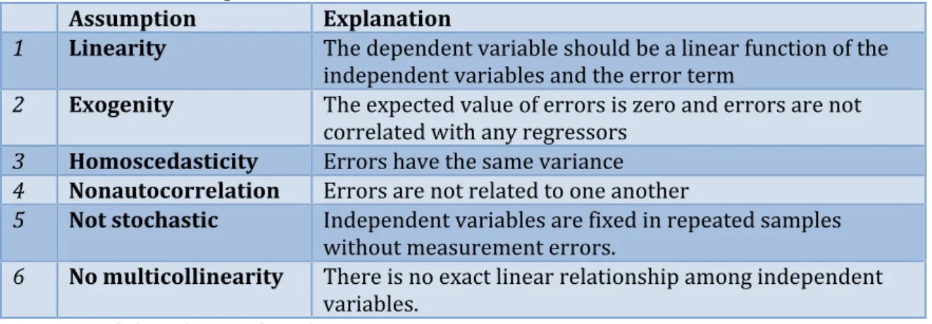
minimize the SSR (Koop, 2013). The OLS regression model is based on several underlying assumptions that is necessary for the model to be valid shown in table 6. More information about the assumptions are found in appendix 2.

Table 2: OLS-Assumptions

Assumption Explanation

1 Linearity The dependent variable should be a linear function of the independent variables and the error term

2 Exogenity The expected value of errors is zero and errors are not correlated with any regressors

3 Homoscedasticity Errors have the same variance 4 Nonautocorrelation Errors are not related to one another

5 Not stochastic Independent variables are fixed in repeated samples without measurement errors.

6 No multicollinearity There is no exact linear relationship among independent variables.

Source: Park (2011), Koop (2013)

3.2.3 Panel Data

Panel data are also called longitudinal or cross-sectional time-series data. They have observations in several different time periods and on the same units (Kennedy, 2008). A panel data set has “multiple entities, each of which has repeated measurements at different time periods (Park, 2011). The data set used in this research can be classified as panel data as the accounting data are from different time periods but at the same



SSR (y_i

i1

n

(33)

time the companies and the variables are the same. The panel dataset used is defined as balanced because the same years are used for each company.

3.2.4 Panel data estimation Methods

Based on the literature, it is common to use panel data estimation methods for data that combines cross-sectional and time-series data. When using penal data there are some assumptions that must be valid for the estimated coefficients to be valid. In this analysis the focus will be on three different methods; pooled ordinary least squares, fixed effects model and random effects model. The assumptions for each method can be found in appendix B.

Pooled OLS

If there is no individual heterogeneity, i.e. no cross-sectional or time specific effect (ui =

0), than ordinary least squares (OLS) provides consistent and efficient parameter estimates to use on panel data (Park, 2011).

Formula 8: Yit = 0 + Xit + it Where:

 Yit: Dependent variable

 0: Intercept

 : Vector of the independent variables coefficient

 Xit: Vector of the independent variable

 it: Error term where ui = 0

If individual effects are not zero in panel data, heterogeneity may influence the assumption of exogenity and nonautocorrelation, and the model will provide biased

(34)

and inconsistent estimators. If this is the case, the fixed effects model and the random effect model provide ways to deal with these problems (Park, 2011)

Fixed Effects Model

The fixed effects (FE) model takes the presence of unobserved heterogeneity into account and divides the error term into two components; one that captures the variation between the different firms analysed (ui) and one that captures the

remaining disturbance (vit). Formula 9: Yit = (0 + ui) + Xit + vit

The fixed effects model controls for any possible correlation among the independent variables and omitted variables by treating ui as a fixed effect. This means that OLS

assumption 2 will not be violated. The fixed effects model is estimated by using least squares dummy variable (LSDV) estimation and a within effect estimation method. Random Effects Model

A random effects model assumes that heterogeneity is not correlated with any regressor and that the error variance estimates are specific to firms. Hence ui is a

component of the composite error term ().

Formula 10: Yit = 0 + Xit + (ui + vit)

The slopes and intercept of regressors will be the same across firms, but the difference between firms will lie in their individual errors and not in their intercepts. The random effects model is estimated by using generalized least squares (GLS) or an OLS

estimator. The difference between them is that the GLS estimator will still be efficient in the presence of autocorrelation and heteroscedasticity, while OLS will not. On the

(35)

Selection of Estimation Model

In order to decide on what estimation model that fits the available data best, the characteristics of the data should be examined. Firstly, the model should be tested for the underlying OLS-assumptions (normality, heteroscedasticity, multicollinearity, autocorrelation), then for panel data effects. If there is a presence of panel data effects, the pooled OLS method should be excluded and random- or fixed estimation models should be used. The Hausman specification test will then be conducted in order to indicate whether the FE- or RE-model is preferred. However Brooks (2008) claims that the random effects model will provide lower volatility and more efficient estimations than the fixed effects model. This is based on the fact that the RE-model utilises the information in the panel data so that the effects of the independent variables on

leverage can be illuminated. Another advantage with the RE-model is that less degrees of freedom is lost because there are less parameters to estimate.

3.3 The Regression Model

A regression is an advanced approach to evaluate the relationship between variables and it is the most common tool used in applied economics (Koop, 2013). The main objective of a regression analysis is to investigate how the value of the dependent variable (Y) changes when the value of one of the independent variables (X1, X2, X3,…,

Xk) changes by one unit. A simple regression model analyses the linear relationship

between two variables, while a multiple regression model take into account that the independent variables can affect each other and jointly affect the dependent variable.

(36)

This paper will use two different models, model 1 is given by book value of leverage as the dependent variable, and model 2 will use market value of leverage as the

dependent variables. Both models will be used along with the determinants discussed in section X as independent variables. Therefore the following general model applies:

Formula 11: blev/mlev = 0 + 1  profit + 2  sizeit + 3  tangit + 4  growit + 5  liqit + 6  ndtsit + it

The reason for using both book value and market value of leverage is to examine if the chosen independent variables affect them differently. While model 1 is based on historic accounting values, model 2 incorporates the expectations of future cash flows. Table 6 shows the variables and the proxies used in this paper. The proxies have been determined based on previous literature, so that it will be easier to compare the results.

Table 3: Variable proxies

Variable Proxy

Book Value of Leverage Total Debt / (Total Debt + Book Value of Equity)

Market Value of Leverage Total Debt / (Total Debt + Market Value of Equity)

Profitability (P) EBITDA/Total Assets

Size (S) Ln (Total Sales)

Tangibility (T) Fixed Assets/Total Assets

Growth (G) Market capitalisation/Book value

Liquidity (L) Tot. Current Assets/Tot. Current Liabilities

Non-Debt Tax Shield (NDTS) Depreciation/Total Assets

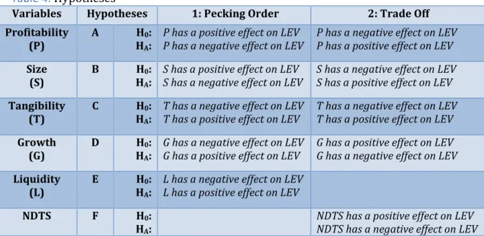
3.4 Hypotheses

Based on the theories presented in chapter 2 and their impact on firms’ capital

(37)

basis of the pecking order theory. The hypothesis testing will be used in order to examine whether one theory is better than the other in explaining the capital structure of Norwegian listed firms. The null hypothesis will be rejected on the 5% significance level.

Table 4:Hypotheses

Variables Hypotheses 1: Pecking Order 2: Trade Off

Profitability

(P) A HHA0: :

P has a positive effect on LEV

P has a negative effect on LEV P has a negative effect on LEV P has a positive effect on LEV

Size

(S) B HHA0: :

S has a positive effect on LEV

S has a negative effect on LEV S has a negative effect on LEV S has a positive effect on LEV

Tangibility (T)

C H0:

HA:

T has a negative effect on LEV T has a positive effect on LEV

Growth (G)

D H0:

HA:

G has a negative effect on LEV G has a positive effect on LEV

G has a positive effect on LEV G has a negative effect on LEV

Liquidity

(L) E HHA0: :

L has a negative effect on LEV L has a positive effect on LEV

NDTS F H0:

HA:

NDTS has a positive effect on LEV NDTS has a negative effect on LEV

(38)

Chapter 4: ANALYSIS

This chapter will begin with a descriptive analysis of the data, then a correlation analysis will be conducted, followed by the choice of estimation model. It will continue presenting the empirical results obtained from analysing the effect different firm-specific

determinants may have on capital structure in listed Norwegian firms. The analysis is based on the specifications discussed in the previous chapter. The findings will then be presented before they are compared and contrasted to the established theories and previous empirical research presented in chapter 2.

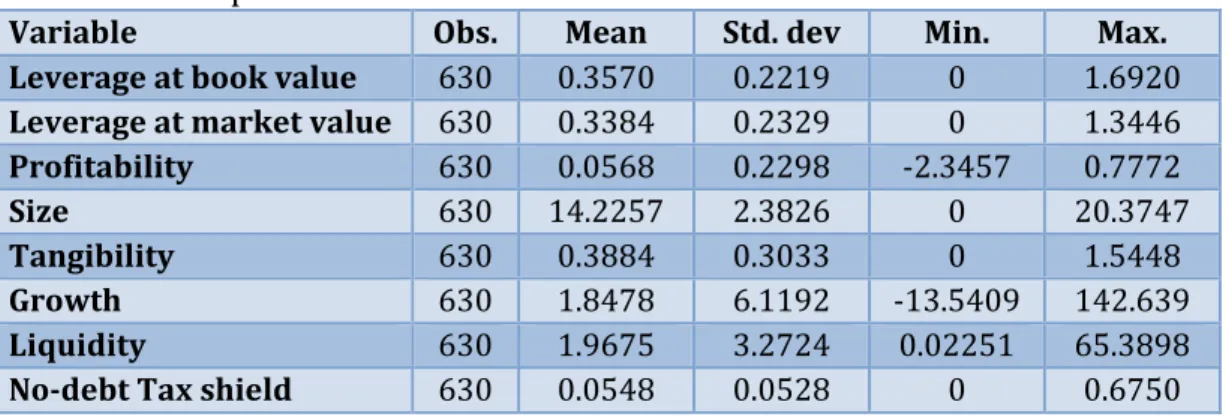
4.1 Descriptive statistics

Descriptive statistics is used to describe the basic features of the data in an empirical research paper. They provide simple summaries about the sample and the measures. Table 6 presents information for 2007-2013 regarding the number of observations, mean, standard deviation and maximum- and minimum values for the variables.

Table 5: Descriptive statistics

Variable Obs. Mean Std. dev Min. Max.

Leverage at book value 630 0.3570 0.2219 0 1.6920

Leverage at market value 630 0.3384 0.2329 0 1.3446

Profitability 630 0.0568 0.2298 -2.3457 0.7772

Size 630 14.2257 2.3826 0 20.3747

Tangibility 630 0.3884 0.3033 0 1.5448

Growth 630 1.8478 6.1192 -13.5409 142.639

Liquidity 630 1.9675 3.2724 0.02251 65.3898

No-debt Tax shield 630 0.0548 0.0528 0 0.6750

Looking at the independent variables, some key values stand out from the table.

(39)

indicate that the dataset should be corrected for extreme values. As the time period studied includes the financial crisis in 2007-08, this may explain some of the outliers, as it does not reflect the true characteristics of firms over time.

The median is the middle observation after the observations have been ranged and is not as sensitive to extreme values as the mean. For book value, the median is 0.336, while it for market value is 0.311 between 2007 and 2013. This suggests that the assets are primarily financed through equity, implying that firms have more equity available to meet their financial obligations. The difference in annual median value for book and market leverage over time is graphically illustrated in figure 5.

Figure 3: Median values of Leverage over time

The above figure show that the median values for book value generally have been larger and less variable than market value over the time period. The explanation lies in market value depending on the market price, which continuously fluctuates and

follows the business cycles. Besides, the market value of shares is usually higher than book value, so the difference between the measurements was expected.

20.00 % 22.50 % 25.00 % 27.50 % 30.00 % 32.50 % 35.00 % 37.50 % 40.00 % 42.50 % 2007 2008 2009 2010 2011 2012 2013 Medi an de bt ratio Year Blev Mlev

(40)

4.1.2 Outliers in the data set

An outlier is generally a data point that is far outside the norm for a variable or

population. The descriptive statistics suggests that it is appropriate to eliminate some outliers in the data, as it can undermine the results of the analysis. According to Osborne and Overbay (2004) the effect of including outliers in the analysis may involve:

1. Increased error variance and reduced explanatory power of statistical tests 2. Decreased normality

3. Biased estimates that may be of substantive interest

There are several different approaches in how to handle the problem with outliers. One can choose to take a passive approach and keep them; alternatively the outliers can be removed or changed. Based on the descriptive statistics, the most significant outliers are removed from the dataset. The outliers are identified in STATA, and then dropped accordingly.

4.1.3 Descriptive statistics after removing outliers

Table 7 presents the descriptive statistics after removing extreme observations in the dataset. The dataset can now be described as unbalanced as removing some

estimations makes for an uneven distribution of N and T. The average value for all the variables remain roughly the same, except for growth and liquidity. These variables had the most significant outliers, so the expected change in mean would therefore also be large. The standard deviation for all the variables have been reduced as the gap between the minimum and maximum values has decreased, but profitability and size also have a slightly more significant change than the other variables.

(41)

Table 6: Descriptive statistics after removal of outliers

Variable Obs. Mean Std. dev Min. Max.

Leverage at book value 587 0.3556 0.2017 0 0.9719

Leverage at market value 587 0.3459 0.2286 0 1.2029

Profitability 587 0.0655 0.1655 -0.9023 0.4910

Size 587 14.3093 2.0045 6.1312 19.9517

Tangibility 587 0.3951 0.3023 0 1.5448

Growth 587 1.5933 1.6584 -0.6249 15.5413

Liquidity 587 1.7166 1.2821 0.0605 8.8682

No-debt Tax shield 587 0.04918 0.03601 0 0.1967

Leverage at Book Value

In the sample, leverage at book value has a mean of 0.3556. This implies that around 35.5% of the average firm’s total assets are financed by debt. Frank and Goyal (2009) got an average leverage at book value of 0.29, which indicates that the companies in this sample are slightly more leveraged than the US companies they researched. However Kouki and Said (2012) got a mean leverage at book value of 0.51 on their study of French firms.

Leverage at Market Value

The average leverage at market value is 0.3459, which indicates that the average company in this sample have a debt level of 34.6% of their market value. In

comparison Frank and Goyal (2009) got a mean of 0.28. The standard deviation of 0.22 is larger than for book value of leverage, which implies that the sample variations are larger than for market value.

Profitability

Profitability have a mean of 6.55% which can be considered considerably higher than the mean of 2% found in the research conducted by Frank and Goyal (2009). However, they used EBITDA/sales as a proxy for profitability. Song (2005) got a profitability

(42)

mean of 8% and a standard deviation of 0.28. Both values a higher than for this sample, indicating that profitability is higher, but with more variability in Swedish firms.

Size

The proxy for size in this sample is the logarithm of sales. As a result, the mean, maximum and minimum statistics makes little economic sense. However a standard deviation of 2.3826 indicates large differences in size between the companies in this sample.

Tangibility

This variable has an average of 0.395. This is slightly higher than the average of 0.35 that Frank and Goyal (2009) discovered in their research. In comparison, Song (2005) got a tangibility ratio mean of 0.288, which is over 0.1 lower than for this sample. Furthermore he got a standard deviation of 0.22, which is significantly lower than the standard deviation of 0.30 from this sample.

Growth

Growth has an average of 1.84, which indicates that the market expects future growth for the companies included in the sample. This is similar to the mean of 1.74 found by Frank and Goyal (2009), but higher than the mean discovered by Song (2005) of 1.07. Liquidity

This variable has a mean of 1.71 and it can be interpreted as how much the average company is able to pay off its obligations. Thus for every 1 of current liabilities, firms have 1.71 of current assets to cover their short-term liabilities. Ozkan (2001) achieved a liquidity ratio of 1.64, which indicates that Norwegian firms are slightly better at

(43)

as the current liabilities will outweigh their current asset. The variable has a standard deviation of 1.28, which is reasonable. The value of the ratio is therefore relatively close around the mean.

Non-Debt tax Shield

Non-debt tax shield has a mean of 0.49. This result is slightly lower compared to a mean of 0.055 obtained from Song (2005). The same applies to the standard deviation from his research, which is 0.048 and about 0.012 higher than what can be detected in this sample.

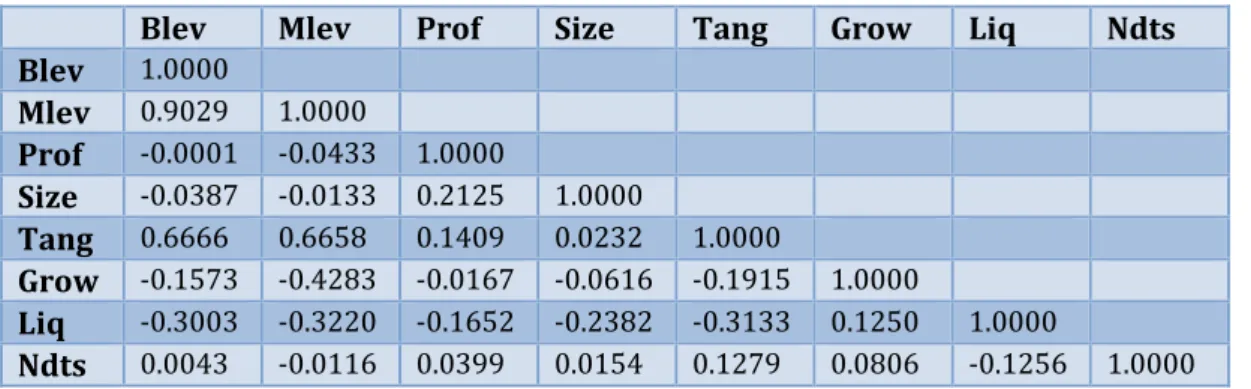
4.2 Correlation analysis

A correlation analysis presents the pair wise correlation between all the variables that are included in the regression analysis. The null-hypothesis is that there is no

correlation between the variables. Table 9 presents the correlation matrix and gives an overview of the correlation coefficient of the variables.

Table 7: Correlation matrix

Blev Mlev Prof Size Tang Grow Liq Ndts

Blev 1.0000 Mlev 0.9029 1.0000 Prof -0.0001 -0.0433 1.0000 Size -0.0387 -0.0133 0.2125 1.0000 Tang 0.6666 0.6658 0.1409 0.0232 1.0000 Grow -0.1573 -0.4283 -0.0167 -0.0616 -0.1915 1.0000 Liq -0.3003 -0.3220 -0.1652 -0.2382 -0.3133 0.1250 1.0000 Ndts 0.0043 -0.0116 0.0399 0.0154 0.1279 0.0806 -0.1256 1.0000

Using panel data for the regression analysis eliminates most of the effect of collinearity between variables. However this will still cause problems if one or more variables are close to perfect collinearity. Table 9 shows that this is not a concern as the correlation

(44)

between most of the variables are relatively low. The correlation between tangibility and the debt measures are moderately correlated, which means that there is a linear relationship between them. As expected, there is strong correlation between book value of leverage and market value of leverage because of the similar definitions.

4.3 Evaluation of Estimation Model

This section will evaluate what estimation model is the most appropriate to use. Firstly a pooled OLS regression analysis will be conducted and the data will be examined to see if it fulfils the assumptions of the discussed estimation models from the previous chapter. Then the sample will be tested for panel data effects to see if panel data estimation methods are more appropriate. All the assumptions will be tested and discussed before the estimation model is chosen.

4.3.1 OLS regression Analysis

An OLS regression analysis was conducted on the two models, one with book value of leverage as the dependent variable and the other with market value of leverage.

Blev = 0 + 1  profit + 2  sizeit + 3  tangit + 4  growit + 5  liqit + 6  ndtsit + it

Mlev = 0 + 1  profit + 2  sizeit + 3  tangit + 4  growit + 5  liqit + 6  ndtsit + it

Table 8: Pooled OLS regression results

Variables 1: Book-value of leverage 2: Market value of leverage

profitability -0.1185557** -0.1945976***

size -0.0065745* -0.0054111

tangibility 0.431606*** 0.4482379***

growth -0.0016718 -0.0403105

liquidity -0.0226829*** -0.0253397***

(45)

F 88.30 131.49

Prob > F 0.0000 0.0000

R-squared 0.4774 0.5767

Adjusted R-squared 0.4720 0.5724

4.2.1.1 ANOVA results

The values for F and Prob > F indicates whether or not the regression model is significant. Specifically, they test the null hypothesis that all of the regression

coefficients are equal to zero. For both models, Prob > F is equal to 0.000, which means that we can reject H0 and conclude that the model is significant. The F-value is the

explained variability divided by the unexplained variability. In these models the F-value is 88.30 and 131.49, respectively. The higher the F-F-value, the more of the total variability is accounted for in the model.

R-squared measures the explanatory power of the model and indicates how the variance in the dependent variable (Y) can be explained by the independent variables (X) (Koop, 2013). The results show that the model with book value as the dependent variable is equal to 0.4720, while using market value gives a significantly higher R-squared of 0.5724. This means that for model 1, 47.20% of the variation in leverage at book value can be explained by the significant independent variables. For model 2, 57.24% of the variation in market value can be explained by the significant

independent variables.

4.2.1.2 Interpretation of coefficients

The table shows that there are some differences in the magnitude of the coefficients between having book value as the independent variable compared market value. When interpreting the coefficients, all other variables are kept constant (ceteris paribus).