Carlos P´erez-Sancho, David Rizo, and Jos´e M. I˜nesta Department of Software and Computing Systems
University of Alicante P.O. box 99, E-03080 Alicante, Spain {cperez,drizo,inesta}@dlsi.ua.es
http://grfia.dlsi.ua.es
Abstract. Music genre meta-data is of paramount importance for the organization of music repositories. People use genre in a natural way when entering a music store or looking into music collections. Automatic genre classification has become a popular topic in music information re-trieval research. This work brings to symbolic music recognition some technologies, like the stochastic language models, already successfully applied to text categorization. In this work we model chord progressions and melodies asn-grams and strings and then apply perplexity and na¨ıve Bayes classifiers, respectively, in order to assess how often those struc-tures are found in the target genres. Also a combination of the different techniques as an ensemble of classifiers is proposed. Some genres and sub-genres among popular, jazz, and academic music have been consid-ered. The results show that the ensemble is a good trade-off approach able to perform well without the risk of choosing the wrong classifier.
1
Introduction
Organization of large music repositories is a tedious and time-intensive task for which music genre is an important meta-data. Automatic genre and style classification have become popular topics in Music Information Retrieval (MIR) research because musical genres are categorical labels created by humans to characterize pieces of music and this nature provides genre with a high semantic and cultural information to the items in the collection.
Traditionally, the research on music genre classification has been divided into the audio [1] and symbolic [2] music analysis and retrieval domains. This work focuses on the symbolic approach, where music is found as digital scores. Language modeling is a common practice in natural language tasks, such as speech recognition [3], and also in text categorization [4]. Our goal is to bring stochastic language models, already applied successfully in text categorization, to music genre classification. Some of those technologies, at least those working at a lexical level, can be transferred to music with some adaptation work.
In a former work [5], we studied how melodies could be coded and classified. Here, we are going to test whether chords can be represented by a model that learns probabilities from the progressions used in each genre.
Little attention has been paid in the genre recognition literature to how har-mony can help in this task. For example, in [6] the authors use pitch histograms as feature vectors (either computed from audio signals or directly derived from MIDI data). In contrast to that low-level harmony features, the representation chosen in this paper is to model higher level harmonic structures, like chord progressions, asn-grams and strings in order to compute how often those struc-tures are found in the target genres. There are a small number of papers in the literature that poses this problem.
To test these models, we have built a classification framework with different genres in order to see whether such a model built from a genre is able to correctly identify new chord sequences belonging to it.
2
Experimental data
Music works from different genres covering a wide range of music areas have been utilized: popular, jazz, and academic music. Popular music data have been separated into three sub-genres:pop,blues, andceltic(mainly Irish jigs and reels). For jazz, three styles have been established: apre-bopclass grouping swing, early, and Broadway tunes,bopstandards, andbossanovasas a representative of latin jazz. Finally, academic music has been categorized according to historic periods: baroque,classicism, andromanticism. All these categories have been defined with the help and advice of music experts that have also collaborated in the task of assigning meta-data tags to the files and rejecting outliers in order to have a reliable ground-truth for the experiments.
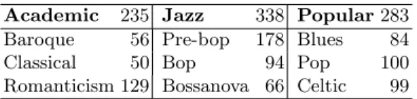
The number of files eventually used for each genre is displayed in Table 1. The total amount of pieces was 856, providing around 60 hours of music data.
Table 1.Number of files per genre and subgenre in the different training sets. Academic 235 Jazz 338 Popular283
Baroque 56 Pre-bop 178 Blues 84
Classical 50 Bop 94 Pop 100
Romanticism 129 Bossanova 66 Celtic 99
The Academic and Jazz corpora have been obtained from sample files for the software ‘Band in a Box’1
. The Popular music files were downloaded from the Internet2
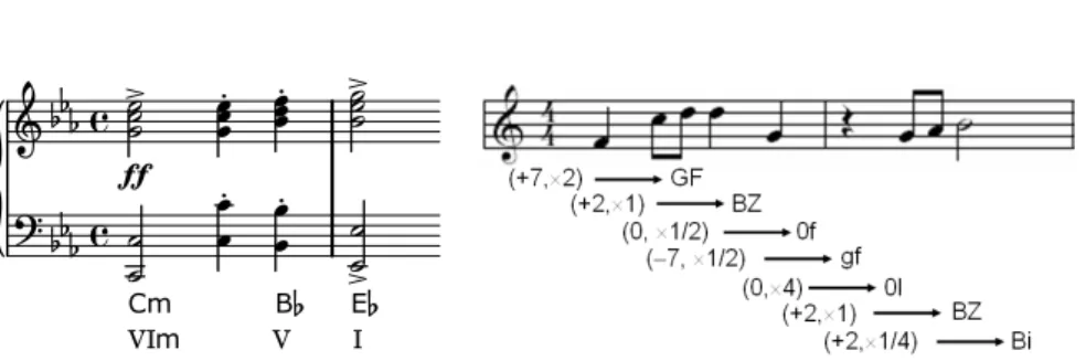
. These data can be obtained upon request to the authors. In order to focus on the chord progressions instead of the chords themselves, all the songs have been transposed to C Major / A minor and the chords are encoded as their degrees for the tonality the score is in. For example, the sequence Cm – B♭– E♭ in Fig. 1-left is coded as VIm – V – I, as it corresponds for the E♭major key.
1
http://www.pgmusic.com (PG Music) 2
ff
Fig. 1.Example of chord encoding (left) and melodic words (right).
The other source of information is the melody, which is represented as a sequence of intervals and duration ratios between consecutive notes (silences are not considered, being like an extension of the former note), that are mapped into sequences of alphanumeric characters (named 2-words, since they are extracted from pairs of notes). See Fig. 1-right for an example.
3
Classification methods
For the experiments in section 4 two statistical classification methods have been used: a na¨ıve Bayes classifier andn-grams. Both of them have been widely used in text classification tasks and, more recently, in music genre classification by melody [5, 7].
Both techniques allow the construction of a statistical model for each genre from a set of documents. While n-grams make use of context information to compute the probabilities for each word, na¨ıve Bayes computes the probability of each word on its own3.
3.1 Na¨ıve Bayes Classifier
The na¨ıve Bayes classifier, as described in [8], has been used. It assumes that all words in a document are independent of each other, and also independent of the order in which they are generated. This assumption is false in our problem and also in the case of text classification, but na¨ıve Bayes can obtain near optimal classification errors in spite of that [9].
We have a set of classesC=
c1, c2, . . . , c|C| . A music piece is represented as
a vectorx∈ {0,1}|V|, where each componentxtrepresents whether the wordwt
appears in the document or not, and|V|is the size of the vocabulary. A document xis assigned to the classcj ∈ Cwith maximum a posteriori probability, in order
to minimize the probability of error: P(cj|x) =
P(cj)P(x|cj)
P(x) . (1)
3
We are using “document” in a metaphoric way for “music piece”, while a “word” can be either a chord or a short melody fragment.
where P(cj) is the a priori probability of classcj, P(x|cj) is the probability of
xbeing generated by classcj, andP(x) =P |C|
j=1P(cj)P(x|cj).
The class-conditional probability of a documentP(x|cj) is given by the
prob-ability distribution of wordswtin classcj, which can be learned from a labelled
training set of melodies, X =
x1,x2, . . . ,x|X | , using a supervised learning
method.
Each class follows a multivariate Bernoulli distribution:
P(x|cj) = |V|
Y
t=1
xtP(wt|cj) + (1−xt)(1−P(wt|cj)) (2)
whereP(wt|cj) are the class-conditional probabilities of each word in the
voca-bulary, and these are the parameters to be learned from the training set. Bayes-optimal estimates for probabilities P(wt|cj) can be easily calculated
by counting the number of occurrences of each word in the corresponding class: P(wt|cj) =
1 +Mtj
2 +Mj
(3) where Mtj is the number of documents in classcj containing wordwt, andMj
is the total number of documents in classcj. Also, a Laplacean prior has been
introduced in the equation above to avoid zero probabilities. Prior probabilities for classes P(cj) can be estimated from the training sample using a maximum
likelihood estimate:
P(cj) =
Mj
|X | (4)
Classification of new documents is performed then using Equation 1, which is expanded using Equations 2 and 4.
Feature selection. A common practice in text classification is to reduce the dimensionality of those vectors, through a feature selection process. This is done by selecting the words which contribute most to discriminate the class of a document, using a ranked list of words extracted from the training set. A widely used measure to rank these words is theaverage mutual information(AMI) [10], which gives a measure of how much information about a class is provided by each single word. Informally speaking, we can consider that a word is informative when it is very frequent in one class and less in the others.
AMI is calculated between 1: the class of a document and 2: the absence or presence of a word in the document. We defineC as a random variable over all classes, and Ft as a random variable over the absence or presence of word wt
in a document, Ft taking on values in ft ∈ {0,1}, where ft = 0 indicates the
absence of wordwtandft= 1 indicates its presence. The AMI is calculated for
eachwt as4: I(C;Ft) = |C| X j=1 X ft∈{0,1} P(cj, ft) log P(cj, ft) P(cj)P(ft) (5) 4
whereP(cj) is the number of documents for classcjdivided by the total number
of documents;P(ft) is the number of documents containing the wordwtdivided
by the total number of documents; andP(cj, ft) is the number of documents in
classcjhaving a valueftfor wordwtdivided by the total number of documents.
3.2 n-grams
In this case, our language model is a probability distribution that assigns a probability to a progression of wordsP(w1, . . . , wk), so that the probability of
each word in the sequence is dependent on its contextP(wi|w1, . . . , wi−1).
Estimating the probabilities of such a model can be an arduous task, and maybe computationally unaffordable, when dealing with long sequences. This is why language models are often approximated using n-gram models. An n -gram is a sequence of n words in which the first n−1 words are considered as the context. Thus, the estimated probability of a word wi given a context
is computed as P(wi|wi−n+1, . . . , wi−1). Note that now we are modeling the
probability of finding a given word after a context ofn−1 words, while formerly we were coding words as symbols in a vocabulary, and probabilities were then estimated for those symbols.
In order to perform genre classification with then-grams, a different language model must be constructed for each genre in the data set. Each sequence (song) in the data set is decomposed inn-grams of a fixed lengthn(see Fig. 2). Then, the probability of each different n-gram is computed as the probability of the last word given its context. This probability can be easily calculated by dividing the number of occurrences of the n-gram by the number of occurrences of its context in the given data set:
P(wi|wi−n+1, . . . , wi−1) = N(wi−n+1, . . . , wi) N(wi−n+1, . . . , wi−1) . (6) Progression: I – V – VI – V – I Bigrams: I – V ; V – VI ; VI – V ; V – I Trigrams: I – V – VI ; V – VI – V ; VI – V – I
Fig. 2.Decomposition of a chord progression in bigrams and trigrams.
Once a language model is constructed for each genre, the probability that a new progressionw=w1, . . . , wk has been generated by modelcis:
Pc(w) = k
Y
i=1
Pc(wi|wi−n+1, . . . , wi−1) . (7)
Thus, a test sample can be classified by following the risk minimization cri-terion, i.e. given the set of classesC={c1, . . . , c|C|}, each test sample is assigned
Parameter smoothing Even when the training set is big enough to build a good language model, there can be situations where we can find words in a test sample that have not been seen previously. When such situation occurs, the probability of then-grams containing those words is zero, thus causing the probability of the whole sequence being zero by the application of Eq. (7).
To avoid this problem, it is common to use a procedure known assmoothing, in which a small probability is substracted from the set of known words, and then shared out among all unseen words. There are several techniques to calculate the optimal amount of probability that must be taken off, and what percentage of it must receive every unseen word.
A similar problem happens when a new sequence of words is found. This can be solved using a process known as backing-off in which the probability of a previously unseen sequence of words can be estimated using a lower order model built using (n−1)-grams. In this work theWitten-Belldiscounting method [11] combined with backing-off has been used.
3.3 Classifier ensembles
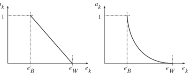
The results for different similarity models may differ substantially. This feature can be exploited by combining the outcomes of individual comparisons. Two weighted voting methods have been utilized. These approaches are described below. e k ek a k ak 1 1 e W e B eB eW
Fig. 3.Different models for giving the authority (ak) to each classifier in the ensemble
as a function of the number of errors (ek) made on the training set.
Best-worst weighted vote (BWWV). In this ensemble, the best and the worst classifiersCk in the ensemble are identified using their estimated accuracy.
A maximum authority,ak= 1, is assigned to the former and a null one,ak = 0,
to the latter, being equivalent to removing this classifier from the ensemble. The rest of classifiers are rated linearly between these extremes (see figure 3-left). The values forak are calculated using the number of errorsek as follows:
ak= 1−
ek−eB
eW −eB
where
eB= min
k {ek} and eW = maxk {ek}
Quadratic best-worst weighted vote (QBWWV). In order to give more authority to the opinions given by the most accurate classifiers, the values ob-tained by the former approach are squared (see figure 3-right). This way,
ak = (
eW −ek
eW −eB
)2
.
Classification. For these voting methods, once the weights for each classifier decision have been computed, the class receiving the highest score in the voting is the final class prediction. If ˆck(xi) is the prediction ofCk for the samplexi,
then the prediction of the ensemble can be computed as ˆ c(x) = arg max j X k wkδ(ˆck(xi), cj) , (8)
beingδ(a, b) = 1 ifa=b and 0 otherwise.
4
Experiments
Experiments were performed at two levels of the genre hierarchy. The first level corresponds to the three music domains considered: academic, jazz, and popular; and the second level to the 9 sub-genres shown in Table 1. In order to build ensembles of classifiers, we need to evaluate first the performance of each single classifier so that they can be properly weighted. For this reason, the data set was randomly split in two: 80% (684 songs) were used in section 4.1 to evaluate the single classifiers and compute their weights, and the remaining 20% (172 songs) were used in section 4.2 to evaluate the performance of the ensembles.
4.1 Evaluation of the single classifiers
In this preliminary stage we wanted to evaluate the performance of the classi-fication methods on two different dimensions of the data set: 1) using the two representations (harmony vs. melody), and 2) looking at the two levels of the genre hierarchy. Besides the 3- and 9-class problems, we also considered the in-tradomain problems, i.e. classifying among the 3 sub-genres within each domain. For this, an experiment was run for each data set, classifier, and encoding. All these experiments were validated using a 10-fold cross-validation scheme. Values ofn={2,3,4}were used for then-gram models.
Table 2 shows the results obtained in these experiments. Note that the best results were obtained when classifying among the three broad domains. In this case the use of harmony is significantly better than using the melodies. When descending to the second level in the genre hierarchy (9-class problem) there were
significant differences between the use of harmony or melody: using melody helps to make better decisions. Although the performance for the 9-class problem is poorer, a 62% in the best case, note that the baseline of the recognition rate is now around 21%. Note also that the deviations for the three sub-problems in the second level of the general hierarchy are much higher than those for the 3-class problems. This shows less consistency in the performance against the different partitions that suggests the presence of outliers. The validity of the ground-truth should be addressed in further works.
Table 2. Average classification percentages and deviations from the 10-fold sub-experiments obtained withn-grams and na¨ıve Bayes.
Chords (harmony) Melodic words
2-grams 3-grams 4-grams MB 2-grams 3-grams 4-grams MB 3 classes 86±3 85±3 85±3 86±4 76±5 80±6 79±5 76±6 9 classes 36±10 38±12 38±15 62±6 55±8 50±8 50±9 55±12 academic 40±20 40±20 40±20 54±14 60±20 60±20 60±20 62±10 jazz 62±7 63±8 63±6 72±7 70±10 54±11 54±11 73±10 popular 56±12 60±9 60±9 85±6 81±6 80±5 81±5 79±6
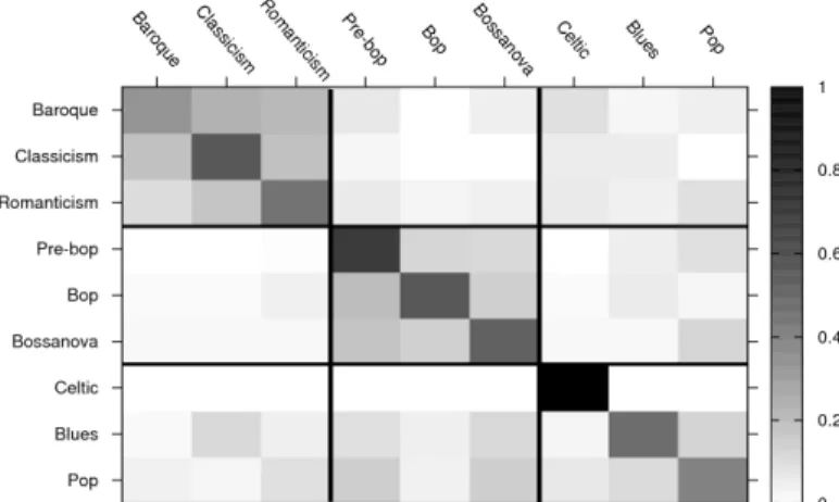
When these results are studied in more detail (see Fig. 4) one sees that the errors mainly occur within the broad domains. Misclassifications among different domains are much less frequent. We can profit from the good results achieved at the 3-classes level in order to improve the performance, by pruning the errors made between different domains using a hierarchical classifier.
Fig. 4.Confusion matrix for the 9-class problem using classification by Bernoulli with na¨ıve Bayes. Grey levels represent the classification percentages. Rows are the ground truth and columns the actual system output. The parts of the matrix corresponding to the different music domains have been highlighted.
4.2 Hierarchical classification
From the analysis of the results obtained in the previous section, we propose a two-level classification scheme. At the first level of the hierarchy, decisions will be made based on harmonic information to distinguish between the academic, jazz, and popular domains. At the second level, three different classifiers will be used, each one trained with the sub-genres belonging to their respective do-mains. At this level we decided to use melodic information because it consistently performed better than using harmony.
At both levels, decisions were made by an ensemble of classifiers, built as explained in section 3.3. This is better than choosing just the classifier which performed the best in the previous step because there is a risk that it will not perform so well with a new data set, given the standard deviations observed in the previous experiment, specially in the intradomain problems.
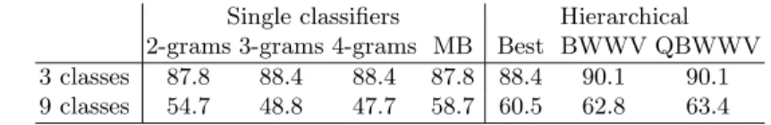
The weights for each classifier in the ensembles were computed using the results shown in Table 2 and the two proposed weighting methods. As a result, we have two hierarchical classifiers, one made up of ensembles using the BWWV voting method, and another using the QBWWV method. Both classifiers were trained using the whole training set, and then evaluated using the remaining 20% of previously unseen files. We also compared this approach with the one using just the classifier which performed the best at each level. Finally, the performance of the individual classifiers was assessed with this validation set, in order to check whether there is a real improvement when using the hierarchical approach. Results of these experiments are shown in Table 3. As it can be seen, all hierarchical classifiers performed slightly better that the best single classifier, with the best results obtained when using ensembles with the QBWWV voting method.
Table 3.Classification percentages at the two levels of the hierarchy using single and hierarchical classifiers.
Single classifiers Hierarchical 2-grams 3-grams 4-grams MB Best BWWV QBWWV 3 classes 87.8 88.4 88.4 87.8 88.4 90.1 90.1 9 classes 54.7 48.8 47.7 58.7 60.5 62.8 63.4
5
Conclusions and future work
In this paper, the feasibility of classifying music in genres using harmonic and melodic information has been tested. For this, we appliedn-gram models and a na¨ıve Bayes classifier on a corpus of music files from three broad genres (aca-demic, jazz, and popular music), and nine sub-genres. Full chord names encoded as degrees with respect to the tonality have been used for encoding chord pro-gressions, whereas pairs of intervals and duration ratios between consecutive notes have been used for melodies.
When classifying the three broad genres we obtained an 86% recognition rate using harmonic information, and comparable results were observed when using both the na¨ıve Bayes classifier andn-gram models. For the nine-subgenre experiment the performance was poorer, but the system was still able to correctly classify close to a 60% of the target samples. Classification errors were mainly made between close sub-genres, inside each of the three domains.
When comparing the performance of the system using harmonic and melodic information better results were obtained by using harmony for distinguishing between the three broad domains, while the use of melodies was of better use for the intradomain problems. Thus, we have proposed a hierarchical (two-level) classification scheme in which decisions are made using harmony and melody in the first and second levels, respectively. At each level, an ensemble of classifiers is used in order to increase system stability. The results obtained with the hier-archical ensembles equalled or outperformed those obtained with the best single classifier in the nine-subgenre problem.
Acknowedgements
The authors want to thank Pedro J. Ponce de Le´on and Jos´e L. Heredia for their help and advice. This work is supported by the Spanish PROSEMUS project (TIN2006-14932-C02) and the research programme Consolider Ingenio 2010 (MIPRCV, CSD2007-00018).
References
1. Tzanetakis, G., Cook, P.: Musical genre classification of audio signals. IEEE Transactions on Speech and Audio Processing10(2002) 205–210
2. McKay, C., Fujinaga, I.: Automatic genre classification using large high-level mu-sical feature sets. In: Proceedings of the ISMIR. (2004) 525–530
3. Jelinek, F.: Statistical Methods for Speech Recognition. MIT Press (1998) 4. Cavnar, W.B., Trenkle, J.M.: N-gram-based text categorization. In: Proceedings
of SDAIR-94, 3rd Annual Symposium on Document Analysis and Information Retrieval, Las Vegas, US (1994) 161–175
5. P´erez-Sancho, C., I˜nesta, J.M., Calera-Rubio, J.: Style recognition through statis-tical event models. Journal of New Music Research34(2005) 331–340
6. Tzanetakis, G., Ermolinskyi, A., Cook, P.: Pitch histograms in audio and symbolic music information retrieval. In: Proceedings of the ISMIR, Paris, France (2002) 7. Cruz-Alc´azar, P.P., Vidal, E., P´erez-Cortes, J.C.: Musical style identification
us-ing grammatical inference: The encodus-ing problem. In: Proceedus-ings of the 8th Iberoamerican Congress on Pattern Recognition, CIARP 2003. (2003) 375–382 8. Mccallum, A., Nigam, K.: A comparison of event models for naive bayes text
classification (1998)
9. Domingos, P., Pazzani, M.: Beyond independence: conditions for the optimality of simple bayesian classifier. Machine Learning29(1997) 103–130
10. Cover, T.M., Thomas, J.A.: Elements of Information Theory. John Wiley (1991) 11. Witten, I., Bell, T.: The zero-frequency problem: Estimating the probabilities
of novel events in adaptive text compression. IEEE Transactions on Information Theory 37(1991) 1085–1094