A Direct Bootstrap Method for Complex Sampling Designs From a Finite Population

A Direct Bootstrap Method for Complex Sampling

Designs From a Finite Population

In complex designs, classical bootstrap methods result in a biased variance estimator when the sampling design is not taken into account. Resampled units are usually rescaled or weighted in order to achieve unbiasedness in the linear case. In the present article, we propose novel resampling methods that may be directly applied to variance estimation. These methods consist of selecting subsamples under a completely different sampling scheme from that which generated the original sample, which is composed of several sampling designs. In particular, a portion of the subsampled units is selected without replacement, while another is selected with replacement, thereby adjusting for the finite population setting. We show that these bootstrap estimators directly and precisely reproduce unbiased estimators of the variance in the linear case in a time-efficient manner, and eliminate the need for classical adjustment methods such as rescaling, correction factors, or artificial populations. Moreover, we show via simulation studies that our method is at least as efficient as those currently existing, which call for additional adjustment. This methodology can be applied to classical sampling designs, including simple random sampling with and without replacement, Poisson sampling, and unequal probability sampling with and without replacement.

KEY WORDS: One–one resampling design; Poisson sampling; Replications; Simple random sampling; Unequal probability sampling; Variance estimation.

1. INTRODUCTION

Resampling methods such as the bootstrap and jackknife are largely used to estimate variances across a broad spec-trum of statistical contexts. In survey sampling, the variances of even simple estimators depend on the sampling design, and can take very complex forms, particularly when the sampling design is elaborate. The classical bootstrap method, developed by Efron (1979) cannot be directly applied to cases of sam-pling from a finite population because the identical and inde-pendent distribution assumption fails under sampling without replacement.Gross(1980) andChao and Lo(1985) have pro-posed a method for variance estimation based on reconstructing artificial populations from the sample. Bootstrap samples are then selected from this artificial population using the original sampling scheme. Another important class of methods arises from the rescaled bootstrap (Rao and Wu 1988) which consists of modifying the sample values of the variable of interest to construct an unbiased estimator of the variance in the linear case. Other methods have also been proposed byMcCarthy and Snowden(1985),Kuk(1989),Rao, Wu, and Yue(1992),Shao and Tu(1995), Sitter (1992a,1992b),Booth, Butler, and Hall

(1994),Holmberg(1998).

In this article, we propose a new methodology that can be applied to classical sampling designs both with and without re-placement, as well as both equal and unequal inclusion proba-bilities. Our methodology consists of selecting bootstrap sam-ples from the original sample in such a way that it eliminates the need for scaling, weighting of the sample, and using artificial populations. We argue that if the aim is variance estimation, the resampling design must be radically different from that which generates the original data. We then proceed to construct an ad hoc resampling design by mixing several designs, such that the

Erika Antal (E-mail:[email protected]) is Doctoral Student and Yves Tillé (E-mail:[email protected]) is Professor, Institute of Statistics, Faculty of Economics, University of Neuchâtel, Pierre à Mazel 7, 2000 Neuchâtel, Switzerland. The authors would like to thank the Editor, associate editor, refer-ees, and Anthea Monod for their insightful comments and propositions which have resulted in significant improvement of this article. This work was sup-ported by Equal Opportunity Office of the University of Neuchâtel.

bootstrap variance is equal to the estimator of the variance in the linear case, and such that the bootstrap sample has the same expected sample size as that of the actual sample size of the data, and can thus be treated as the original sample. This fea-ture is particularly attractive because imputation, weighting for nonresponse, and calibration can thus be carried out without the need for any additional considerations or corrective techniques. In sampling without replacement, the main idea consists in se-lecting bootstrap samples by mixing sampling with and with-out replacement in order to reproduce a variance estimator that comprises the finite population correction.

The remainder of the article is structured as follows. We will first review basic notions of the theory of survey sampling, and provide an overview of the most frequently used sampling de-signs. We will then introduce two new sampling designs, sim-ple random sampling with over-replacement and one–one re-sampling, that are used exclusively in resampling. We will then define sufficient conditions for a direct unbiased estimator for the variance of the total in resampling designs, and provide the construction of the algorithms used to draw such samples for several basic sampling designs. Finally, we supplement the the-oretical proofs with results of simulation studies performed on several functions of interest, including the total, the median, the Gini index, and the ratio of totals. These results are compared to those obtained under resampling methods currently used, such as the classical bootstrap with and without replacement. We conclude with comparative remarks on our proposed method-ology, and propose additional development and future research on the topic.

2. SAMPLING DESIGN AND ESTIMATION Consider the finite populationU= {1, . . . ,k, . . . ,N}and the variable of interest y that takes the value yk on unit k, for allk in U. A first aim is to estimate the total of the interest variable: Y =_k∈Uyk. A random sample is a random vec-torS=(S1, . . . ,Sk, . . . ,SN), whereSk is the number of times

unit k isselectedinthesample.Ifthesampleisselected with-outreplacement,then Skcanonlytakethevalues0and1.Ifthe samplehasafixedsamplesize n,then _k∈USk=n.

LetπkbetheexpectationofSk,thatis,πk=E(Sk).Thejoint

expectationof twounits kand isπk=E(SkS).Moreover, k=cov(Sk,S)=πk−πkπ.If the sample is selected with-out replacement,πk is the inclusion probability of unitkand

πkis the joint inclusion probability of unitkand.

Ifπk>0,for allk∈U,then the totalY can be estimated in

an unbiased manner by using the Horvitz–Thompson estimator Y=_k∈USkyk/πk.The variance ofYis

var(Y)= k_∈U _∈U yky πkπ k. (1)

Theoretically, ifπk>0,for allk=∈U, this variance can be estimated in an unbiased manner by

var(Y)= k∈U ∈U SkSyky πkπ k πk . (2)

Nevertheless, this variance estimator is often very unstable. It can even take negative values. When the sampling design has a fixed sample size, then the variance can be written

var(Y)=−1 2 k∈U ∈U yk πk − y π 2 k,

and, if πk>0, for all k=∈U, can be estimated by the Yates–Grundy estimator of variance:

var(Y)=−1 2 k∈U ∈U SkS yk πk− y π 2 k πk . (3)

Expression (3) holds for sampling with or without replacement and can also be written in the quadratic form

varD(Y)= k∈U ∈U SkSyky πkπ Dk, (4) with Dk= ⎧ ⎪ ⎪ ⎪ ⎪ ⎨ ⎪ ⎪ ⎪ ⎪ ⎩ − j∈U j=k Sjkj πkj ifk= k πk ifk=. (5)

When the sampling design with or without replacement has a fixed sample size, estimator (3) must be preferred to estima-tor (2). We shall show below in Result2that the presentation of estimator (3) in a quadratic form is needed to construct a re-sampling method that produces an unbiased estimator.

3. BASIC SAMPLING DESIGNS

In aPoisson sampling designwith inclusion probabilitiesπk,

theSk areNindependent Bernoulli random variables with pa-rameterπk.Thus,k=πk(1−πk)ifk=and 0, if not. So k/πk=1−πkifk=and 0 if not.

Simple random sampling with replacementis very common. The sampling design is given by Pr(S=s)=N−n_s1···skn_···sN,

for alls∈Rn,whereRn= {s∈Nn|

N

k=1sk=n}.It follows thatk= −n(N−1)/{N2(N−1)}whenk=∈Uandkk=

n(N−1)/N2 when k∈U. Since the sample size is fixed, we can construct an unbiased estimator by using the quadratic form based on theDk, defined in Expression (5),Dk= −1/(n−1) whenk=∈U, andDkk=1 whenk∈U, which gives

var(Y)=N 2 n 1 n−1 k∈U Sk(yk−Y)2, (6) whereY=n−1k_∈USkyk.

Unequal probability with replacement with fixed sample size, is a generalization of simple random sampling with re-placement to unequal probabilities of selection. The distribution of this sampling design is multinomial:

Pr(S=s)= n s1· · ·sk· · ·sN ₋1 k∈U πk n sk for alls∈Rn.

In unequal probability sampling with replacement,

k= n(N−1) N2 × ⎧ ⎪ ⎪ ⎨ ⎪ ⎪ ⎩ πk 1−πk n ifk= −πkπ n ifk=.

In order to construct an unbiased estimator of the variance, we can use the Dk defined in Expression (5), and we get Dk= −1/(n−1)whenk=∈U, andDkk=1 whenk∈U. Curiously, Dk does not depend on the πk’s of the sampling

design and are the same as simple random sampling with re-placement. The unbiased variance estimator (3) becomes

var(Y)= n n−1 k∈U Sk yk πk− Y n 2 . (7)

Simple random sampling without replacementis defined by the following sampling design: Pr(S=s)=N_n−1, for alls∈ Sn,where Sn= s∈ {0,1}N N k=1 sk=n. .

We thus havek= −n(N−n)/{N2(N−1)}whenk=∈U, kk=n(N−n)/N2whenk∈U,k/πk= −(N−n)/{N(n− 1)}whenk=∈U,andkk/πkk=(N−n)/Nwhenk∈U.

Unequal probability sampling without replacementand with fixed sample size is much more complex. The first problem is that there are many methods of sampling without replace-ment and with unequal probabilities. Each method provides a specific matrix of joint inclusion probabilities. These in-clusion probabilities are, however, very similar if the sam-pling has a large entropy (Berger 1998; Brewer and Donadio 2003; Henderson 2006), such as the random systematic de-sign (Madow 1949) or the Rao–Sampford design (Rao 1965; Sampford 1967), the Brewer design (Brewer 1975), the maxi-mum entropy design or the random pivotal design (Tillé 2006, pp. 79–95 and p. 106). The second problem is that these inclu-sion probabilities can never be simplified. So, a simpler expres-sion of variance than (1) and its estimator (2) cannot be con-structed. Several approximations of variance based on a simple sum have been proposed, however. These approximations are obviously biased, but simulations have shown that they have

smaller mean squared errors than estimators (2) and (4) (Hájek 1981; Matei and Tillé 2005). There are thus various ways to estimate the variance. The strictly unbiased estimator consists of computing theDk by expression (5). A general biased and simple estimator of variance is given by

var(Y)= k∈S ck yk πk − k∈Sckyk/πk k_∈Sck 2 ,

where theck are weights that we discuss further. This expres-sion can be viewed as an approximation of the Dk given in expression (5), by Dk= ⎧ ⎪ ⎪ ⎪ ⎨ ⎪ ⎪ ⎪ ⎩ ck− c 2 k j∈USjcj ifk= −ckc j∈USjcj ifk=.

Diverse values have been proposed for theck:

1. A simple value was given byHájek(1981), who proposed using

ck1=

n

n−1(1−πk). (8)

2. Deville and Tillé(2005) proposedcksuch that

ck2−

c2_k2

j∈USjcj2 =

1−πk. (9)

In this case, the diagonal elementsDkk2 of the approx-imated matrix are equal to 1−πk. A solution does not always exist for this equation, for instance whenn=2.

3. One could also take thecksuch that

ck3− c2_k3 j∈USjckj = − j∈U j=k Sjkj πkj, (10)

but this approximation needs to solve a nonlinear system of equations. In this case, the diagonal elements of the approximated matrix Dkk3= − j∈U j=k Sjkj πkj

and correspond to the diagonal of the matrix used for the Yates–Grundy estimator of variance given in (5).

Simple random sampling with over-replacement was re-cently proposed byAntal and Tillé(2010). The sampling de-sign is defined by Pr(S1=x1, . . . ,SN=xN)=(cardRn)−1=

N+n−1

n

−1

. The N+_nn−1 samples with replacement have ex-actly the same probability of being selected. The marginal dis-tribution ofSkis given by Pr(Sk=j)= N+n−1 n ₋1 × N−1+n−j−1 n−j , j=0, . . . ,n,

which is an inverse hypergeometric distribution.The expecta-tion is E(Sk)=n/N,and the matrix ofkis given by

k= (N−1)(N+n)n N2_(N+1) × ⎧ ⎨ ⎩ 1 ifk= − 1 N−1 ifk=. This design has a larger variance than sampling with replace-ment and will be used only for resampling.

4. RESAMPLING AND SUFFICIENT CONDITIONS Define the random setS that contains the list of labels for the units selected in the sampleS. If a unit is selected several times in the sample, the labels can appear several times inS.

For instance, if from populationU= {1,2,3,4,5,6},we select a sampleSthat takes the value(0,2,1,0,3,1), the setStakes the value{2,2,3,5,5,5,6}. A resampling method is a second stage on sampling from sampleS. A subsampleS∗=(S∗_k,k∈S)

can thus be presented as a sequence of discrete nonnegative random variables S∗_k that denote the number of times unit k

is resampled. For example, if, in the above example,S∗ takes the values(1,0,3,0,2,0,1), then the subsample setS∗will be

{2,3,3,3,5,5,6}. TheS∗_kare generally not independent. A cor-relation is indeed necessary to obtain an unbiased estimation of the variance when the sample size is fixed. The resampling sam-ple size is denoted byn∗.

In fact, a resampling method is a second phase of sam-pling that can depend on the first phase. Let E∗(·)=E(·|S), var∗(·)=var(·|S) and cov∗(·,·)=cov(·,·|S) denote, respec-tively, the conditional expectation, variance and covariance un-der the resampling design with respect to the original design. Moreover, let Pr∗(·)=Pr(·|S)denote the probability under the resampling design and conditionally to the original design. Let αk =E∗(S∗_k), αk=E∗(S∗_kS∗) and cov∗(S_k∗,S∗)=k = αk−αkα.The resampled estimator of the total is defined as Y∗=_k∈SykS∗_k/πk.This estimator is generally biased, its

con-ditional expectation is E∗(Y∗)= k_∈S ykE∗(S∗_k) πk = k_∈S ykαk πk . (11)

Note thatαkcan depend onS. Ifαk=1,then the estimator is

unbiased.

The conditional variance of the resampled estimator is var∗(Y∗)= k∈S ∈S yky πkπ k. (12)

This directly leads to two fundamental results:

Result 1. A sufficient condition for E∗(Y∗)=Y is αk=1,

for allk∈U.

This result directly comes from the equality between Expres-sion (11) and the Horvitz–Thompson estimator.

Result 2. A sufficient condition for var∗(Y)=var(Y), is

k=k/πk,for all k, ∈U and a sufficient condition for var∗(Y)=varD(Y),isk=Dk,for allk, ∈Uif the sample size is fixed.

Thisresultdirectlycomesfromtheequalitybetween Expres-sions(2)and(12)orbetweenExpressions (4)and(12)when thesamplesizeofSisfixed.

Infact,themainideaofthisarticleistodevelopresampling methodsthatsatisfyconditionsgiveninResults 1 and 2. This idealeadsustochooseasamplingdesignforS∗that is com-pletelydifferentfromthesamplingdesignusedfor S.Indeed, Result1isgenerallynotsatisfiedbyusingthesamesampling designfor S and S∗,becausekand Dkareofverydifferent natures:thek arevariancesandcovariances,buttheDkare not.

Letθ be an estimator of a function of interest θ. Estima-torθ is a function of the observed data {(yk, πk),k∈S}. The

bootstrap estimatorθ∗ is the same function asθ, applied on the bootstrap data{(yk, πk),k∈S∗}. Practically, a sequence of

bootstrap samplesS∗1, . . . ,S∗mare selected with the bootstrap design. The bootstrap variance given in (12) is approximated by

var∗(θ∗)= 1 m−1 m j=1 (θ_j∗−θ )2,

whereθ_j∗ is the bootstrap estimator computed on thejth boot-strap sample andθ=(1/m)m_j=1θ_j∗.

5. THE SIMPLEST EXAMPLE: RESAMPLING FROM A POISSON SAMPLE

In a Poisson sampling design,k/πk=0 whenk=∈U, andkk/πkk=1−πkwhenk∈U.The resampling design must

be such that E∗(S∗_k)=1,var∗(S∗_k)=1−πk,and cov∗(S∗_k,S∗)=

0, for allk=.Algorithm1can be used to generate suchS∗_k’s. The main idea consists of selecting a part of the units without replacement and a part with replacement with Poisson random variables in order to reproduce the finite population correction 1−πk.

With Algorithm 1, the expectations, variances and co-variances of the S∗_k can be computed E∗(S∗_k)=E∗(S∗_kA)+

E∗(S∗_kB) =πk +1 ×(1 −πk)= 1. Moreover, var∗(S∗_k) =

E∗[var∗(S∗_k|S∗_kA)] +var∗[E∗(S∗_k|S∗_kA)] =1−πk.This bootstrap

method provides the exact Horvitz–Thompson estimator in the linear case. Indeed, var∗(Y∗)= var∗(_k∈SykS∗_k/πk) =

k∈Sy2k(1−πk)/π

2

k =var(Y).

6. THE ONE–ONE RESAMPLING DESIGN The one–one design is a sampling design defined only for re-sampling. It is an ad hoc construction used to randomly selectn

units from a sample of sizenin such a way that the expectation and the variance ofS∗_k are equal to 1, that is, E∗(S∗_k)=1 and var∗(S∗_k)=1.This sampling design is a mixture between a sim-ple random sampling with replacement and a simsim-ple random Algorithm 1Resampling procedure for Poisson sampling Define, independently, fork∈S:

• S∗_kAis a Bernoulli random variable with parameterπk. • IfS∗_kA=1 thenS∗_kB=0,

else S∗_kB is a Poisson random variable with parameter

λ=1.

• The resampling design isS∗_k=S∗_kA+S∗_kB.

Algorithm 2The one–one resampling design

• Ifn=2,then S∗1= 0 with probability 1/2 2 with probability 1/2 andS∗₂=2−S∗₁. • Ifn≥3,then – Compute: m= 1 2 1+ 4n2_+5n−1 n−1 , (13) wherexis the largest integer less than or equal tox

and

α=m(n−1)(m+1)−n(n+1)

2m(n−1) . (14)

– Define the random variable

˜ n=

m with a probabilityα m+1 with a probability 1−α.

– Select a simple random sample with overreplacement with sample size n˜ from S. This sample is denoted byS_kA∗ .

– Select a simple random sample with replacement with sample size n− ˜n from S. This sample is denoted by

S∗_kB. This second sample is independent from the first one.

– The final sample isS∗_k=S∗_kA+S∗_kB.

sampling with over-replacement. Its implementation is given in Algorithm2.

Result 3. IfS∗_k is the number of times unitkis selected by the one–one resampling design described in Algorithm2, then E∗(S∗_k)=1,var∗(S∗_k)=1,cov∗(S_k∗,S∗)= −1/(n−1), for all

k=.

Proof. The case wheren=2 is obvious. For the case where

n≥3,we have that E∗(S∗_k|˜n)=E∗(S_kA∗ |˜n)+E∗(S∗_kB|˜n)= ˜n/n+ (n− ˜n)/n=1.Thus E∗(S∗_k)=E∗E∗(S∗_k|˜n)=1.Moreover,

var∗(S∗_k|˜n)=var∗(S∗_kA|˜n)+var∗(S∗_kB|˜n) =(n−1)(n+ ˜n)n˜ n2_(n+1) + (n− ˜n)(n−1) n2 =n−1 n2 (n+ ˜n)n˜+(n+1)(n− ˜n) (n+1) . Since E∗(S∗_k|˜n)=1, var∗(S∗_k)=E∗var∗(S∗_k|˜n) =αn−1 n2 (n+m)m+(n+1)(n−m) (n+1) +(1−α)n−1 n2 × (n+m+1)(m+1)+(n+1)(n−m+1) (n+1) =(n−1)[n+n2+m(1−2α+m)] n2_(1+n) . (15)

By plugging the value ofα given in (14) and the value ofm

given in (13) in Expression (15), we get var∗(S∗_k)=1. This sampling design has a fixed sample size, which implies that

k∈Scov∗(S∗k,S∗)=cov∗(n,S∗)=0.Moreover, since all the units are treated symmetrically cov∗(S∗_k,S∗)= −var∗(S∗_k)/(n−

1). We thus have k = −1/(n−1) when k=∈ U and kk=1 fork∈U.

7. RESAMPLING FROM A SIMPLE RANDOM SAMPLE WITH REPLACEMENT

7.1 The Usual Bootstrap With Replacement

If the sampleSis selected by means of simple random sam-pling with replacement, the formula of the estimated variance of the total estimator is already given in Expression (6). The usual bootstrap consists of selecting a sample fromS with the same sampling design, that is, a simple random sampling design with replacement fromS. In this case, the variance of the resampled estimator is var∗(Y∗)=(N2/n2)_k∈S(yk−Y)2.The bootstrap variance slightly underestimates the unbiased estimator given in Expression (6). Indeed,var(Y)=n/(n−1)×var∗(Y∗). Ac-tually, this underestimation is not very important if the sample size is large but can create problems if the samples are selected in strata with small sample sizes. Obviously, a correction fac-tor can be applied in each stratum, but these procedures require a particular treatment of the bootstrap sample in each stratum. 7.2 Bootstrap by Using the One–One Sampling Design

The one–one simple random sampling design allows us to avoid the use of correction factors for the variance. Indeed, if the bootstrap sample is selected by a one–one design then the bootstrap variance is var∗(Y∗)= [N2/{n(n−1)}]_k∈S(yk− Y)2.In a one–one simple random sampling, the repetition of the units is slightly larger than with simple random sampling with replacement, which increases the variance by a factor of

n/(n−1).It is thus no longer necessary to multiply the boot-strap variance by this factor.

8. RESAMPLING FROM A SAMPLE SELECTED WITH UNEQUAL PROBABILITIES WITH REPLACEMENT 8.1 The Usual Bootstrap With Replacement

If the sample is selected with unequal probabilities, with re-placement and with fixed sample size, the estimator of variance is given in (7). In this case, the matrix ofDk given in (5) does not depend on theπk’s, which means that the resampling design

must be done with equal selection probabilities. A usual design consists of resampling by means of simple random sampling with replacement, which gives the bootstrap variance

var∗(Y∗)= k∈S yk πk − Y n 2 .

With simple random sampling with replacement, the bootstrap variance thus suffers from a small underestimation. This prob-lem can be annoying when the sample size is small and can be fixed by using a one–one simple random sampling.

8.2 Bootstrap by Using the One–One Sampling Design If the bootstrap samples are selected with a one–one design, the bootstrap variance becomes

var∗(Y∗)= n n−1 k∈S yk πk − Y n 2 ,

and is exactly equal to the estimator of variance (7). The one– one design is thus a convenient design for resampling from a sample selected with unequal probabilities with replacement, particularly when the sample size is small.

9. RESAMPLING FROM A SIMPLE RANDOM SAMPLE SELECTED WITHOUT REPLACEMENT

9.1 Resampling Using Simple Random Sampling With Replacement

In simple random sampling without replacement, the estima-tor of variance is var(Y)=N 2_(N−n) nN 1 n−1 k_∈S (yk−Y)2. (16)

A simple way of resampling consists of using a simple ran-dom sampling with replacement as a resampling design. In this case, var∗(Y∗)=(N2/n2)_k∈S(yk−Y)2.Obviously, the boot-strap variance is not equal to the variance estimator. Indeed,

var(Y)=var∗(Y∗)(N−n)n/{N(n−1)},which means that the resampling variance does not take into account the loss of one degree of freedom and the finite population correction. The bootstrap variance must be corrected by a factor. This correc-tion can become intricate if a large number of samples are se-lected in strata.

9.2 Resampling Using a With Replacement and a One–One Design

In order to avoid the use of a correction factor, one can use a mixture of a simple sampling without replacement and a one– one design as described in Algorithm3in order to directly re-produce the unbiased estimator of variance for the totals.

Result4gives the properties of Algorithm3.

Result 4. If Algorithm3 is used for the resampling design, (i) E∗(S∗_k)=1, (ii) var∗(S∗_k)=(N−n)/N, (iii) cov∗(S_k∗,S∗)= −(N−n)/{N(n−1)}.

Proof. The case wheren−n2/N<2 is trivial. For the case where n−n2/N≥2, the expectation is given by E∗(S∗_k)=

E∗(S_kA∗ )+E∗(S∗_kB|S_kA∗ )Pr∗(SkA=0)=n/N+1×(1−n/N)=

1. Next, the variance is var∗(S∗_k) = E∗[var∗(S∗_k|S∗_kA)] +

var∗[E∗(S∗_k|S∗_kA)] =var∗(S∗_kB|S_kA∗ =0)Pr∗(S∗_kA=0)=1−n/N.

Finally, the covariances can be derived from the symmetry of treatment of the units, which implies that cov∗(S∗_k|S∗_kA,S∗_A)= −var∗(S∗_k)/(n−1)= −(N−n)/{N(n−1)}.

If Algorithm3is used, the resampling variance is thus var(Y∗)=N2N−n nN 1 n−1 k_∈S (yk−Y)2,

and is exactly equal to the estimator of variance given in Ex-pression (16).

Algorithm 3Resampling using a with replacement and a one– one design

• Ifn−n2/N<2:

– With a probabilityq=n(N−n)/(2N), select randomly without replacement and with equal probabilities two units inSdenoted byiandj. Next defineS∗_i =2,S_j∗=

0,Sk=1,for allk∈ {i,/ j}.

– With a probability 1−q,S∗_k=1,for allk∈S. • Ifn−n2/N≥2: – Define m= ⎧ ⎪ ⎪ ⎪ ⎨ ⎪ ⎪ ⎪ ⎩ n2 N with probabilityq n2 N +1 with probability 1−q, whereq= n2/N +1−n2/N.

– Select a sampleS∗_kA fromS with simple random sam-pling design without replacement with a sample sizem. – From the set of units of S such that S∗_kA=0, select a sampleS∗_kBaccording to a one–one design, soS∗_kBhas sizen−m.

– The resampling design isS∗_k=S∗_kA+S∗_kB.

10. RESAMPLING FROM A SAMPLE SELECTED WITH UNEQUAL PROBABILITIES

WITHOUT REPLACEMENT

Unequal probability without replacement is obviously a more complicated problem. The main reason is that the unbiased es-timators given in (2) and (4) of the variance can never been sim-plified, which makes it necessary to compute all the joint inclu-sion probabilities to estimate the variance. When the entropy of the sampling design is large, biased estimators given in (8), (9), and (10) have a smaller mean square error than estimators (2) and (4) (see Matei and Tillé2005). For this reason, we do not propose using a bootstrap method that exactly reproduces the estimator of variance, but rather one that gives one of the three approximations. These methods are described in Algorithms4

and5.

Result5gives the properties of Algorithm4.

Result 5. If Algorithm4is used for the resampling design, (i) E∗(S∗_k)=1, (ii) var∗(S∗_k)=1−φk, (iii) cov∗(S∗_k,S∗)= −q(1−φk1−φ1+φk1)/(n−m1−1)−(1−q)(1−φk2−

φ2+φk2)/(n−m2−1).

Proof. First, the conditional expectation is given by E∗(S∗_k| mj)=E∗(S∗_kA|mj)+E∗(S∗_kB|mj)=φkj+1×(1−φkj)=1.Thus, E∗(S∗_k)=E∗E∗(S_k∗|m)=1. Next, the conditional variance is var∗(S∗_k|mj)=E∗[var∗(S∗_k|S_kA∗ ,mj)|mj] +var∗[E∗(S∗_k|S_kA∗ ,mj), mj] = var∗(S∗_kB|S∗_kA = 0,mj)Pr∗(S_kA∗ =0|mj)= 1−φkj,j =

1,2.Thus, var∗(S∗_k)=E∗var∗(S∗_k|m)+var∗E∗(S∗_k|m)=q(1−

φk1)+(1−q)(1−φk2)=1−φk. Finally, the covariance is

given by

cov∗(S∗_k,S∗|mj)

=cov∗E∗(S_k∗|S∗_kA,S∗_A,mj),E∗(S∗|S∗_kA,S∗_A,mj)|mj +E∗[cov∗(S∗_k,S∗|S∗_kA,S∗_A,mj)|mj]

Algorithm 4 Resampling for unequal probability sampling without replacement: Case 1

Case 1:n−_k∈Sφk≥2.

• Select a sampleS∗_kAwithout replacement with unequal in-clusion probabilitiesφk (the choice ofφkis discussed

be-low) and fixed sample size. This sampling design is the same as the original design. Ifn∗=_k∈Sφkis not an

in-teger, then define

m=

m1= n∗ with probabilityq

m2= n∗ +1 with probability 1−q, whereq= n∗ +1−n∗.Also defineφk1andφk2as the inclusion probabilities such that

k∈S φk1=m1, k∈S φk2=m2, qφk1+(1−q)φk2=φk for allk∈S.

Letφk1andφk2also be the joint inclusion probabilities of the design where sample sizesm1orm2were selected.

• From the set of units ofSsuch thatS∗_kA=0, select a sample

S∗_kBaccording to a one–one design.

• The resampling design isS_k∗=S∗_kA+S∗_kB.

=cov∗(S∗k,S∗|SkA∗ =0,S∗A=0,mj) ×Pr∗(S∗kA=0,S∗A=0|mj) = − 1

n−mj−1×(1−φkj−φj+φkj). Thus

cov∗(S∗_k,S∗)=E∗cov∗(S∗_k,S∗|m)+cov∗[E∗(S∗_k|m),E∗(S∗|m)] = − q n−m1−1× (1−φk1−φ1+φk1) − 1−q n−m2−1× (1−φk2−φ2+φk2). We have seen that according to the definition of theck, there are several ways to approximate the matrix ofDk by a matrix ofDk. The values ofφkthat reconstruct as best as possible the three approximations for ck given in (8), (9), and (10) can be chosen by taking 1−φk=Dkk. Obviously, these resampling

Algorithm 5 Resampling for unequal probability sampling without replacement: Case 2

Case 2:n−_k∈Sφk<2.

• Compute(ψk,k∈S)=1−H(1−φk,k∈S;2)andq= (n−_k∈Sφk)/2.

• With a probabilityqselect a sample without replacement denoted by S∗_kA of size n−2 from S by using inclusion probabilitiesψk.Letψk denote the joint inclusion prob-ability of this design. From the two remaining units, se-lect a one–one design denoted byS∗_kB.The final sample is

S∗_kA+S∗_kB.

variances are not exactly equal to the estimator of variance, but they take into account the correction for finite population. Moreover, the diagonal terms are exactly the same as usual es-timators of variance.

The case wheren−_k∈sφk<2 must also be treated.

Con-sider the procedure used to compute the inclusion probabilities from a vector of positive valuesxk.First, compute the quantities

nxk

∈Ux

, (17)

k=1, . . . ,N. For units for which these quantities are larger than 1, setπk=1.Next, the quantities are recalculated using

(17) restricted to the remaining units. This procedure is repeated until eachπkis in]0,1]. Someπk are 1 and others are propor-tional to xk. LetH(x1, . . . ,xN;n)denote the function that al-lows us to construct these inclusion probabilities from a vector of positive values(x1, . . . ,xN). FunctionH(·; ·)allows us to de-fine Algorithm5in order to select the bootstrap sample in the case wheren−_k∈sφk<2.

With Algorithm5, E∗(S∗_k)=1 and var∗(S∗_k)=(1−ψk)(n− k∈Sφk) 2 and cov∗(S∗k,S∗)= (1−ψk−ψ+ψk)(n− k∈Sφk) 2 .

The φk can be chosen according to the three approximations given above in (8), (9), and (10).

11. MONTE CARLO SIMULATION STUDY FOR NUMERICAL COMPARISONS

First, we developed simulations for matrix reconstruction in order to confirm the theoretical results obtained in Section10

on the new bootstrap methods for unequal probability sampling. As seen earlier, we distinguished the two cases depending on whethern−_k∈Sφkis greater than or equal to 2 or less than 2.

We generated a population for each of these cases. We com-puted the matrices of Horvitz–Thompson and of Yates–Grundy variance estimators, as well as their approximations, we then ran sets of simulations to obtain the matrices of the variances using the new bootstrap method. We noticed that these matrices were very close to the respective approximations, so the method should provide estimators of variance that are very similar to the estimators given by the approximations. In order to be concise, we do not include the results of these simulations in this article. Secondly, we also ran a set of simulations for the vari-ance estimators in different sampling designs. In each case a population of 150 units was generated from the modelyk= (β0+β1x1_k.2+σ εk)2+c, whit xk = |ik| and ik ∼N(0,7), εk∼N(0,1)andσ =15. The regression parameters areβ0= 12.5, β1 =3 and c=4000. The model and its parameters were chosen intentionally to have a distribution forysimilar to a lognormal—as it is often used for income distributions—with a correlated and positive explanatory variablexin the regres-sion model. From this population, 1000 samples were drawn with a sample sizen=50. We knowingly used a large sample rate n/N=1/3 and a skewed population in order to better il-lustrate the performance of the tested bootstrap methods. From each of these samples, we calculated four statistics: the total,

the median, the Gini index of variableyand the ratio of total of variableyon the total of variablex.

Three sampling designs were tested: Poisson sampling, sim-ple random sampling without replacement and a maximum en-tropy design with unequal inclusion probabilities. Concerning the inclusion probabilities, they were calculated proportional to the values of a variablez, which was generated from equation

z=y0.2pwherep∼lnN(0,0.25). In this manner the correla-tion betweenyandzis about 0.5. In the case where the total was the function of interest, the goal was to reproduce the estimator of variance of the total. In fact, for the estimation of the total, estimators of variance can directly be computed. A resampling method is thus not necessary. However, simulations were also run in this case in order to test the performance of the methods. From each of the 1000 initial samples, 1000 bootstrap sam-ples were selected by means of five different bootstrap methods. Besides the new bootstrap method, four other resampling meth-ods were tested. The first one is the bootstrap with replacement proposed byMcCarthy and Snowden (1985) for which a cor-rection factor for the finite population is used. The second one is the bootstrap without replacement, which consists of creat-ing an artificial population from the initial sample and draw-ing bootstrap samples with the same design as the initial one (Gross 1980; Chao and Lo 1985). In the cases of simple random sampling without replacement or unequal inclusion probability sampling design as initial sampling designs, the third method is the rescaled bootstrap ofRao and Wu(1988). For the Pois-son sampling design, we used thePatak and Beaumont(2009) method. Nonlinear functions of interest were also tested: the ra-tio of two totals, the median, and the Gini index. For these func-tions of interest, the variances under the simulafunc-tions, say the Monte Carlo variances, were considered as the true variances of the estimators. In the case where the total was the function of interest, the results were directly compared with the variance of the total that can be exactly computed, and not with the Monte Carlo simulation variance. After drawing the bootstrap samples, the estimators, their variances and the means of these variances were computed for each of the initial samples and were then compared with the approximations of the true variances. Note that the median is not a smooth function of the total. Estimating its variance can therefore be difficult, but the simulations show that in this case bootstrap methods perform well.

In order to measure the performance of the new method and compare it with the other ones, the following five indicators were used:

• Lower error rate (L) in %

L=100 sim sim i₌1 I[θ−1.96× var(θ∗) > θ],

whereI[a] =1 if a is true andI[a] =0 elsewhere,

• Upper error rate (U) in %

U=100 sim sim i=1 I[θ+1.96× var(θ∗) < θ],

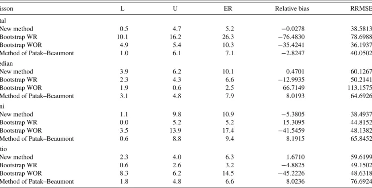
Table 1. Performance of resampling methods in Poisson sampling

Poisson L U ER Relative bias RRMSE Total New method 0.5 4.7 5.2 −0.0278 38.5813 Bootstrap WR 10.1 16.2 26.3 −76.4830 78.6988 Bootstrap WOR 4.9 5.4 10.3 −35.4241 36.1937 Method of Patak–Beaumont 1.0 6.1 7.1 −2.8247 40.0502 Median New method 3.9 6.2 10.1 0.4701 60.1267 Bootstrap WR 2.3 4.3 6.6 −12.9935 50.2141 Bootstrap WOR 1.9 0.6 2.5 66.7149 113.1575 Method of Patak–Beaumont 3.1 4.8 7.9 8.0193 64.6926 Gini New method 1.1 9.8 10.9 −5.3805 38.4937 Bootstrap WR 0.0 5.2 5.2 15.3095 44.8152 Bootstrap WOR 3.5 13.9 17.4 −41.5459 48.1382 Method of Patak–Beaumont 0.6 8.8 9.4 8.1915 65.8452 Ratio New method 2.3 4.0 6.3 1.6710 59.6199 Bootstrap WR 0.6 2.6 3.2 −4.8825 49.1502 Bootstrap WOR 8.3 6.2 14.5 −45.2226 48.6318 Method of Patak–Beaumont 1.8 4.8 6.6 8.0236 76.6924

• Total error rate (ER) in %

ER=100−100 sim sim i=1 Iθ−1.96× var(θ∗)≤θ ≤θ+1.96× var(θ∗), • Relative Bias RB=100×var(θ ∗_)−var sim(θ ) varsim(θ ) =100× B varsim(θ ) , • Relative Root Mean Squared Error

RRMSE=100× !

B2_+var[var(θ∗_)] varsim(θ )

.

The RB gives a measure of the bias of the estimator of variance. The RRMSE measures its accuracy. TheError Ratesallow us to evaluate the capacity of the methods to provide a valid in-ference. The lower and the upper error rates give us an idea of how skewed the distribution of the estimatorθ is. Tables1,2, and3present the numerical performances of the estimators of variance for the three sampling designs, the four functions of interest and the four resampling methods.

Table1 presents the outcomes achieved using the Poisson sampling design with inclusion probabilities proportional to variable z. The variance estimator provided by the proposed method is unbiased for the total and for the other considered function, it is nearly unbiased according to the MC simulation. The relative bias are small, even for the Gini index (around

−5%). For the total and the ratio, the total error rates are about 5%, and for the two other functions of interest about 10%. The bootstrap with replacement is clearly inefficient for the total. In fact, despite the use of a correction factor, the bootstrap with replacement with fixed sample size cannot catch the variance due to the randomness of the sample size of the Poisson

sam-pling design. The variance estimator can thus largely underes-timate the true variance. For the other functions of interest, the bootstrap with replacement provides a relatively high coverage rate, but the estimators themselves are biased. With regard to the bootstrap without replacement, the variance estimators are also strongly biased. For the total, the Gini index and the ra-tio, the variance estimators underestimate the true variance, and give lower coverage rates. For the median, the coverage rate is 97.5% which is only due to the large overestimation of the vari-ance. In general, the performance of the proposed method and the method ofPatak and Beaumont(2009) are equivalent. The estimators are unbiased, or have a slight bias for each func-tion. The RRMSE have the same order and the error rates show a slightly positively skewed distribution, with coverage rates between 90 and 95%. We can conclude that the new method provides essentially the same results as the others, but its appli-cation is simpler: it does not require a correction factor, rescal-ing or artificial population.

Table2 shows the results of the applications of resampling methods for simple random sampling without replacement. Here, the original sampling design has a fixed sample size, which explains why the bootstrap with replacement method performs better. Instead of the method of Patak and Beau-mont(2009) dedicated to Poisson sampling, we have used the rescaled bootstrap proposed byRao and Wu(1988). The sim-ulations show that, for the total error rates, the bootstrap with replacement method performs slightly better than the three oth-ers, but the coverage rates provided by these others are also between 93% and 94% for each function of interest. The lower and upper error rates for each method and for each function of interest show the same behavior: the distributions are skewed right. There are small biases, positive in the case of the total, the median and the ratio of two totals, except for the rescaled bootstrap method, where the variance of the median is under-estimated. For the Gini index, the first three methods give an

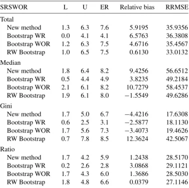
Table 2. Performance of resampling methods in simple random sampling without replacement sampling design

SRSWOR L U ER Relative bias RRMSE Total New method 1.3 6.3 7.6 5.9195 35.9356 Bootstrap WR 0.0 4.1 4.1 6.5763 36.3808 Bootstrap WOR 1.2 6.3 7.5 4.6716 35.4567 RW Bootstrap 1.0 6.5 7.5 0.6130 33.0132 Median New method 1.8 6.4 8.2 9.4256 56.6512 Bootstrap WR 0.5 4.4 4.9 3.8235 49.2184 Bootstrap WOR 2.1 6.1 8.2 10.7279 58.4537 RW Bootstrap 1.9 6.1 8.0 −1.5549 49.6286 Gini New method 1.7 5.0 6.7 −4.4216 17.6308 Bootstrap WR 0.6 2.5 3.1 −2.5877 18.1130 Bootstrap WOR 1.7 5.6 7.3 −3.4073 19.4626 RW Bootstrap 0.7 7.8 8.5 12.3624 42.5067 Ratio New method 1.7 4.2 5.9 1.2438 28.5170 Bootstrap WR 0.2 2.6 2.8 3.0868 29.1121 Bootstrap WOR 1.7 4.3 6.0 1.3686 28.5030 RW Bootstrap 1.8 4.8 6.6 0.0379 27.1146

estimator that underestimates the true variance, in contrast to the rescaling bootstrap method. In general, for simple random sampling without replacement, there is no crucial difference in performance between the resampling methods. They all pro-vide a slightly biased estimator, with relatively high coverage rates—around 94%—and the variabilities of the variance esti-mators are also similar.

Table3shows the performance of resampling methods under a maximum entropy design with inclusion probabilities

propor-Table 3. Performance of the resampling methods in maximum entropy sampling design

UPWOR L U ER Relative bias RRMSE Total New method 0.4 7.4 7.8 −0.9515 35.8027 Bootstrap WR 0.0 2.8 2.8 6.8616 34.9417 Bootstrap WOR 3.1 8.8 11.9 −22.6490 33.1929 RW Bootstrap 2.8 10.6 13.4 −36.7334 49.8869 Median New method 3.5 6.8 10.3 0.9405 58.6158 Bootstrap WR 1.3 5.0 6.3 −12.9157 48.5572 Bootstrap WOR 0.2 0.0 0.2 233.5629 280.1593 RW Bootstrap 16.6 19.0 35.6 −71.0074 72.6283 Gini New method 2.1 5.6 7.7 −3.8518 7.1675 Bootstrap WR 1.0 3.1 4.1 −12.9006 5.5983 Bootstrap WOR 1.3 5.2 6.5 −1.2589 3.3370 RW Bootstrap 7.7 16.7 24.4 −64.8759 65.8130 Ratio New method 2.6 3.6 6.2 −2.3080 36.2905 Bootstrap WR 1.2 1.5 2.7 1.0800 30.9940 Bootstrap WOR 2.0 0.7 2.7 41.4054 53.3239 RW Bootstrap 15.3 13.5 28.8 −71.3400 71.9911

tional to variablez. In the proposed bootstrap method, the sec-ond approximation (9) is used, which gives usφk=πk. In the case where the function of interest is the total, the new method gives an unbiased estimator with a coverage rate of 92.2%. The bootstrap with replacement method provides a lower er-ror rate and thus a higher coverage rate. However it is due to a larger estimated confidence interval caused by a slight over-estimation of the variance. The bootstrap without replacement method with an artificial population and the rescaling boot-strap method strongly underestimate the variance and conse-quently give a smaller coverage rate. The RRMSE are essen-tially the same, and again, the distributions of the estimators are skewed right. Concerning the median, the variance estimator of the new method is unbiased while the bootstrap with replace-ment method, and the rescaled bootstrap method underestimate the variance. The bootstrap without replacement method over-estimates it. For the Gini index, the new method and the boot-strap without replacement method perform almost identically: the estimators of the variance are slightly biased (1%–3% in absolute value as relative bias) with a coverage rate of around 92%–93%. The coverage rate provided by the bootstrap with replacement method is larger, but the variance estimator is bi-ased. The rescaled bootstrap method strongly underestimates the variance, which is the reason why the error rate is higher. Concerning the ratio, the estimator under the new resampling method has a small negative bias. In contrast, the bootstrap with replacement method gives an unbiased estimator and the boot-strap without replacement method gives a variance estimator that is 41% larger than the true variance. To summarize these results: the new method performs at least as well as the other methods considered. At the same time, it is simpler and does not require any additional calculation to estimate the variance of the estimators.

These simulations show that the new bootstrap method works at least as well as the usual bootstrap methods. In Poisson sam-pling design, the inefficiency of the bootstrap with replacement is clear. It is due to the randomness of the sample size. In gen-eral, the new method provides an unbiased or a slightly biased estimator with a coverage rate between 89% and 95% for each of the functions of interest under each sampling design consid-ered. Besides having at least the same performance as the other methods, the main advantage of the new method is that it does not require rescaling, correction factors or an artificial popu-lation. Thus, the samples can be directly used to compute the variance of the functions of interest.

12. DISCUSSION

The main idea driving the new methodology presented in this article is that if the original sample is drawn with replacement, the one–one sampling design can be directly used in the boot-strap method even if the units are selected with unequal prob-abilities. If it is drawn without replacement, the variances are smaller than that of a design with replacement and thus a por-tion of the resampled units are selected without replacement and another is selected according to a one–one design in order to achieve the correct variance. The implementation of select-ing resampled units accordselect-ing to a mixture of samplselect-ing designs is straightforward and extremely rapid. It consists in computing the sample sizes of the different components of the mixtures,

andthenproceedstoselectthebootstrapsamples,whichdonot need to be rescaled.The Horvitz–Thompson weightsremain unchangedfromtheoriginalsample.

The simulations show that the classical bootstrapwith re-placement is not appropriate under unequal probability sam-pling without replacement, or if the sample size is random. For simple random sampling without replacement, bootstrap withreplacementrequiresarescalingfactor.Theclassof meth-odsbasedontheconstructionofartificialpopulationshas lim-itations in its time-consuming execution dueto its intricacy. In addition, inaccuracymay arise due to rounding problems arisingfromthemultiplicationofsample unitsbytheinverse oftheirinclusionprobabilitieswhicharealmostneverinteger (Holmberg1998).Thisproblemisbypassedinthe methodol-ogy proposed in the present work. Regarding the method of

Raoand Wu(1988),the bootstrapvaluesneed not be values fromtheoriginalsamplebecauseoftheredefinitiontechnique; althoughthisindeedprovides unbiasedestimators,difficulties mayariseincasesofcalibration,reweighting,andimputation.

ThemethodofPatakandBeaumont(2009)entails noninte-gerweightsthatmayevenbenegative,whichcanleadto boot-strap estimationsthat arenot intuitive. Thisproblem is miti-gatedviaarescalingmethod,butrequiresarescalingfactorfor thevariance,whichalsopresentsdifficultiesunderimputation, calibration,andweightingfortotalnonresponse.Thework pro-posedherecanbeseenasavariantofthemethodofPatakand Beaumont (2009),butweimposeweightsthatarepositiveand integer.

The useof artificial populationsproduces the correct vari-ance,but,asshowninsimulationstudies,canbecumbersome andtimeconsuming.Thepresentworkavoidsthesedifficulties andattainsbootstrapsamplesinadirectmannerthathave pre-ciselythesameweightsas intheoriginalsample,anddonot presentany of the previous limitationswhen weighting, cali-brationorimputationisrequired.

[ReceivedDecember2009.RevisedDecember2010.] REFERENCES

Antal, E., and Tillé, Y. (2010), “Simple Random Sampling With Over-Replacement,” JournalofStatisticalPlanningandInference, 141, 597–601.

[536]

Berger, Y. G. (1998), “Variance Estimation Using List Sequential Scheme for Unequal Probability Sampling,”Journal of Official Statistics, 14, 315–323. [535]

Booth, J. G., Butler, R. W., and Hall, P. (1994), “Bootstrap Methods for Finite Populations,”Journal of the American Statistical Association, 89, 1282– 1289. [534]

Brewer, K. R. W. (1975), “A Simple Procedure forπpswor,”Australian Journal of Statistics, 17, 166–172. [535]

Brewer, K. R. W., and Donadio, M. E. (2003), “The High Entropy Variance of the Horvitz–Thompson Estimator,”Survey Methodology, 29, 189–196. [535]

Chao, M.-T., and Lo, S.-H. (1985), “A Bootstrap Method for Finite Population,”

Sankhy¯a, Ser. A, 47, 399–405. [534,540]

Deville, J.-C., and Tillé, Y. (2005), “Variance Approximation Under Balanced Sampling,”Journal of Statistical Planning and Inference, 128, 569–591. [536]

Efron, B. (1979), “Bootstrap Methods: Another Look at the Jackknife,”The Annals of Statistics, 7, 1–26. [534]

Gross, S. T. (1980), “Median Estimation in Sample Surveys,” inProceedings of the Survey Research Section, American Statistical Association, pp. 181– 184. [534,540]

Hájek, J. (1981), Sampling From a Finite Population, New York: Marcel Dekker. [536]

Henderson, T. (2006), “Estimating the Variance of the Horvitz–Thompson Es-timator,” MSc thesis, School of Finance and Applied Statistics, The Aus-tralian National University. [535]

Holmberg, A. (1998), “A Bootstrap Approach to Probability Proportional-to-Size Sampling,” inProceedings of the Section on Survey Research Methods, American Statistical Association, pp. 378–383. [534,543]

Kuk, A. Y. C. (1989), “Double Bootstrap Estimation of Variance Under System-atic Sampling With Probability Proportional to Size,”Journal of Statistical Computation and Simulation, 31, 73–82. [534]

Madow, W. G. (1949), “On the Theory of Systematic Sampling, II,”Annals of Mathematical Statistics, 20, 333–354. [535]

Matei, A., and Tillé, Y. (2005), “Evaluation of Variance Approximations and Estimators in Maximum Entropy Sampling With Unequal Probability and Fixed Sample Size,”Journal of Official Statistics, 21 (4), 543–570. [536,

539]

McCarthy, P. J., and Snowden, C. B. (1985), “The Bootstrap and Finite Pop-ulation Sampling,” technical report, Public Health Service Publication. [534,540]

Patak, Z., and Beaumont, J.-F. (2009), “Generalized Bootstrap for Prices Sur-veys,” inProceedings of the 57th Session of the International Statistical Institute, Durban, South Africa. [540,541,543]

Rao, J. N. K. (1965), “On Two Simple Schemas of Unequal Probability Sam-pling Without Replacement,”Journal of the Indian Statistical Association, 3, 173–180.

Rao, J. N. K., and Wu, C. F. J. (1988), “Resampling Inference for Complex Survey Data,”Journal of American Statistical Association, 83, 231–241. [534,540,541,543]

Rao, J. N. K., Wu, C. F. J., and Yue, K. (1992), “Some Recent Work on Resam-pling Methods for Complex Surveys,”Survey Methodology, 18, 209–217. [534]

Sampford, M. R. (1967), “On Sampling Without Replacement With Unequal Probabilities of Selection,”Biometrika, 54, 499–513. [535]

Shao, J., and Tu, D. (1995),The Jacknife and Bootstrap, New York: Springer-Verlag. [534]

Sitter, R. R. (1992a), “Comparing Three Bootstrap Methods for Survey Data,”

Canadian Journal of Statistics, 20, 135–154. [534]

(1992b), “A Resampling Procedure for Complex Survey Data,” Jour-nal of the American Statistical Association, 87, 755–765. [534]