STATISTICAL METHODS FOR EVALUATING
BIOMARKERS SUBJECT TO DETECTION LIMIT
by
Yeonhee Kim
B.S. and B.B.A., Ewha Womans University, Korea, 2001
M.S., North Carolina State University, 2005
Submitted to the Graduate Faculty of
Department of Biostatistics
Graduate School of Public Health in partial fulfillment
of the requirements for the degree of
Doctor of Philosophy
University of Pittsburgh
2011
UNIVERSITY OF PITTSBURGH DEPARTMENT OF BIOSTATISTICS
This dissertation was presented by
Yeonhee Kim
It was defended on May 26, 2011 and approved by
Lan Kong, Ph.D., Assistant Professor, Department of Biostatistics, Graduate School of Public Health, University of Pittsburgh
Andriy Bandos, Ph.D., Research Assistant Professor, Department of Biostatistics, Graduate School of Public Health, University of Pittsburgh
Jong-Hyeon Jeong, Ph.D., Associate Professor, Department of Biostatistics, Graduate School of Public Health, University of Pittsburgh
(Joyce) Chung-Chou Ho Chang, Ph.D., Associate Professor, School of Medicine, University of Pittsburgh
Dissertation Director: Lan Kong, Ph.D., Assistant Professor, Department of Biostatistics, Graduate School of Public Health, University of Pittsburgh
STATISTICAL METHODS FOR EVALUATING BIOMARKERS SUBJECT TO DETECTION LIMIT
Yeonhee Kim, PhD University of Pittsburgh, 2011
As a cost effective diagnostic tool, numerous candidate biomarkers have been emerged for different diseases. The increasing effort of discovering informative biomarkers highlights the need for valid statistical modeling and evaluation. Our focus is on the biomarker data which are both measured repeatedly over time and censored by the sensitivity of given assay. Inappropriate handling of these types of data can cause biased results, resulting in erroneous medical decision.
In the first topic, we extend the discriminant analysis to censored longitudinal biomarker data based on linear mixed models and modified likelihood function. The performance of biomarker is evaluated by area under the receiver operation characteristic (ROC) curve (AUC). The simulation study shows that the proposed method improves both parameter and AUC estimation over substitution methods when normality assumption is satisfied for biomarker data. Our method is applied to the biomarker study for acute kidney injury patients. In the second topic, we introduce a simple and practical evaluation method for censored longitudinal biomarker data. A modification of the linear combination approach by Su and Liu [1] enables us to calculate the optimum AUC as well as relative importance of measurements from each time point. The simulation study demonstrates that the proposed method performs well in a practical situation. The application to real-world data is provided. In the third topic, we consider censored time-invariant biomarker data to discriminate time to event or cumulative events by a particular time point. C-index and time dependent ROC curve are often used to measure the discriminant potential of survival model. We extend
these methods to censored biomarker data based on joint likelihood approach. Simulation study shows that the proposed methods result in accurate discrimination measures. The application to a biomarker study is provided.
Both early detection and accurate prediction of disease are important to manage serious public health problems. Because many of diagnostic tests are based on biomarkers, discovery of informative biomarker is one of the active research areas in public health. Our method-ology is important for public health researchers to identify promising biomarkers when the measurements are censored by detection limits.
TABLE OF CONTENTS
PREFACE . . . x
1.0 INTRODUCTION . . . 1
2.0 LITERATURE REVIEW. . . 4
2.1 Classification methods . . . 4
2.2 Statistical methods for censored data . . . 7
2.3 Evaluation of biomarker . . . 8
2.3.1 ROC curve . . . 9
2.3.2 Predictiveness curve . . . 13
2.3.3 C-index . . . 14
2.3.4 Time dependent ROC analysis . . . 16
3.0 DISCRIMINANT ANALYSIS FOR CENSORED LONGITUDINAL BIOMARKER DATA . . . 19
3.1 Introduction . . . 19
3.2 Method . . . 21
3.2.1 Linear mixed model for biomarker data . . . 21
3.2.2 Discriminant analysis . . . 23
3.2.3 Evaluation of classification performance . . . 24
3.3 Simulation study . . . 26
3.4 Application to BioMaRK study . . . 31
3.5 Discussion . . . 34
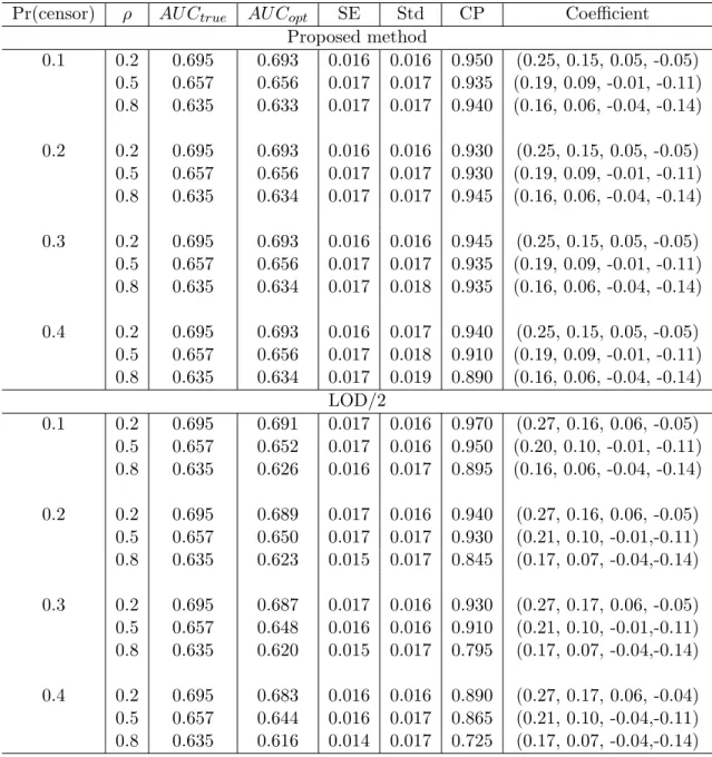
4.0 BEST LINEAR COMBINATION FOR LONGITUDINAL BIOMARKER DATA . . . 37
4.1 Introduction . . . 37
4.2 Method . . . 39
4.2.1 Best linear combination of longitudinal biomarker data . . . 39
4.2.2 AUC estimation for the best linear combination . . . 40
4.3 Simulation study . . . 42
4.4 Application to GenIMS study . . . 46
4.5 Discussion . . . 48
5.0 DISCRIMINATION MEASURE OF CENSORED BIOMARKER FOR SURVIVAL OUTCOME . . . 50
5.1 Introduction . . . 50
5.2 Method . . . 52
5.2.1 Survival model with censored covariates . . . 52
5.2.2 C-index . . . 54
5.2.3 Cumulative/dynamic time dependent ROC . . . 56
5.3 Simulation . . . 58
5.4 Application to BioMaRK study . . . 59
5.5 Discussion . . . 64
6.0 CONCLUSION . . . 66
LIST OF TABLES
1 Concept of sensitivity and specificity . . . 9 2 Parametric estimation of AUC: Comparison of the discriminant ability between
proposed method (PM) and substitution methods (φ2 = 0.5, φ4 = -1.0, σ2 = 1.0) . . . 28 3 Nonparametric estimation of AUC: Comparison of the discriminant ability
between proposed method (PM) and substitution methods (φ2 = 0.5,σ2 = 1.0) 29 4 Performance measures and fit statistics from different models . . . 30 5 Parameter estimates and standard errors from the linear mixed models for
NGAL and HA . . . 34 6 Optimum AUC for the best linear combination of longitudinal biomarker
mea-surements that are generated from the random intercept model. . . 43 7 Optimum AUC for the best linear combination of longitudinal biomarker
mea-surements that are generated from the random intercept and slope model. . . 45 8 Comparison of C-index estimated from the proposed method (PM) and
substi-tution methods (LOD, LOD/2) assuming exponential distribution for survival time (µ= 0, β0 = 0, β1 = 1) . . . 60 9 Comparison of C-index estimated from the proposed method (PM) and
substi-tution methods (LOD, LOD/2) assuming Cox proportional hazard model for survival time (µ= 0, β = 1) . . . 61 10 Comparison ofAU C(t) estimated from the proposed method (PM) and
substi-tution methods (LOD, LOD/2) assuming exponential distribution for survival time . . . 62
11 Comparison ofAU C(t) estimated from the proposed method (PM) and substi-tution methods (LOD, LOD/2) assuming Cox proportional hazard model for survival time . . . 63
LIST OF FIGURES
1 Biomarkera shows the perfect accuracy whereas d shows the worst accuracy. 10 2 Biomarker 1 is more predictive than biomarker 2. . . 13 3 Boxplots of the log transformed NGAL and HA by recovery status . . . 32 4 ROC curve (left) and predictiveness curve (right) for NGAL and HA.. . . 35 5 Boxplots for log transformed IL-6 and D-dimer by survival and mortality groups 47
PREFACE
I would like to thank my family - mom, dad, JongHoon, MinYoung, Charlotte and Banibani for their love.
My advisor, Professor Lan Kong, deserves much gratitude for her constant guidance and men-toring. Also I want to thank my committee members, Dr.Bandos, Dr.Chang and Dr.Jeong, for their time and insight.
I am also thankful to the Clinical and Translational Science Institute for supporting my study.
1.0 INTRODUCTION
Biomarkers are measurable factors that can be used as an indicator of disease or a progres-sion of disease. For example, cholesterol level works as a risk predictor of vascular disease, and serum creatinine is a surrogate for renal disease progression. Due to a biomarkers’ cost-effective benefit for the diagnosis and prognosis of acute and chronic diseases, discovery of a new biomarker is one of the active areas in medical research. Researchers have developed several evaluation tools for biomarker discovery. Diagnostic measures quantify biomarker’s ability of discrimination. It focuses on whether the biomarker can separate patients into event/non-event group. On the other hand, prognostic measures indicate biomarker’s pre-dictive capacity of disease occurrence. The risk can be expressed as a function of biomarker through a statistical model such as logistic regression or Cox proportional hazard model.
Biomarker data are collected from many different procedures, designs and sampling schemes. For instance, biomarkers can be collected only at one time point, or collected repeatedly over several time points. Regardless of the data structure, it is tempting to use only the most recent data in the analysis because of a complexity in handling longitudinal data. Besides the high dimensionality of longitudinal data, analysis of biomarker data be-comes more complicated if some measurements are censored. The censoring occurs due to a limit of detection (LOD). In this case, only measurements which lie between lower and upper detection limits are observable.
We encountered longitudinal censored data from two biomarker studies: The Genetic and Inflammatory Markers of Sepsis (GenIMS) study and the Biological Markers of Recovery for the Kidney (BioMaRK) study. The GenIMS study is a multicenter, cohort study of 2320 patients with community acquired pneumonia (CAP) followed over time. The CAP is the most common cause of sepsis that can lead to death. A set of biomarkers were measured
daily for a week or longer during the hospitalization. One of the goals of this study was to find the relationship between pathways of biomarkers and the risk of sepsis and death. Be-cause of the sensitivity of the assays used to measure the biomarkers, concentration of some biomarkers was below the detectable limit, resulting in a portion of unquantifiable data. The BioMaRK study was conducted as a part of a large randomized clinical trial [2], and enrolled patients who have a renal-replacement therapy for acute kidney injury. The acute kidney injury is a clinically challenging problem for both physicians and patients. Although it is directly related to the health care cost and well-being of patients, effective treatment of acute kidney injury is still not available. Hence, many clinical studies were initiated to explore informative biomarkers for the outcome of renal function. In BioMaRK study, multi-ple plasma and urinary biomarkers are measured repeatedly, and the measurements of some biomarkers are censored due to detection limits. In the previous analysis of longitudinal data, it was common to analyze the biomarker at each time point separately. Censored data were usually deleted or substituted by LOD or LOD/2 with the justification that it is easy to implement and widely understood [3]. However, investigators are frequently in-terested in longitudinal performance of biomarkers. Furthermore, disregarding the censored data often causes significant biases in the estimates of the fixed effects and variance com-ponents, inaccurate estimates of summary statistics, and inaccuracies in risk assessments [4] [5]. The objectives of our research are (1) to develop a classification method for the longitudinal biomarkers subject to left or right censoring due to lower or upper detection limit, and (2) to evaluate the censored biomarker performance for both binary and survival outcomes. The organization of the dissertation is as follows. In chapter 2, we review the models for longitudinal data and existing methods for handling censored data. Underlying theory on the classification method is introduced, followed by statistical evaluation tools for binary and survival outcomes. Chapter3contains the classification methods for longitudinal censored data. In chapter 4, we present how to incorporate the longitudinal biomarkers in the ROC analysis for both censored and non-censored cases. In chapter 5, we change the outcome of interest from binary data to survival data. With the baseline censored biomarker measurements, we calculate the discrimination accuracy for survival outcome by modifying
the original estimation methods for time dependent ROC and C-index. In chapter 6, we close the dissertation with summary on the proposed methods and discussion about future extensions.
2.0 LITERATURE REVIEW
2.1 CLASSIFICATION METHODS
Linear discriminant analysis (LDA) and logistic regression are two standard statistical meth-ods for classification. They are similar in terms of comparing the posterior probabilities that a subject is from groupk (Groupk) when deciding a group membership. Suppose biomarker
Y from Groupk is an n×1 vector of observations with mean µk and covariance matrix Σk.
The πk is the prior probability of a subject belonging to Groupk (k = 0, 1). LDA assumes
that biomarker data follow a normal distribution with common covariance matrix, Σ0 = Σ1
=Σ. The probability density function of Y from Groupk is
fk(Y) = 1 (2π)n/2|Σ|1/2exp [ −(Y −µk)tΣ−1(Y −µk) 2 ] .
Using the Bayes’s rule, the posterior probability of Groupk is calculated as
P r(Groupk|Y) =
fk(Y)πk
f0(Y)π0+f1(Y)π1.
Two posterior probabilities are compared in a log scale so that the log ratio of posterior probabilities leads to an equation linear in Y [6]. We call it as a discriminant function of LDA. Because when Σ0 = Σ1 = Σ,
logP r(Group1|Y) P r(Group0|Y) =logf1(Y) f0(Y) +logπ1 π0 =logπ1 π0 − 1 2(µ 1 +µ0)tΣ−1(µ1−µ0) +YtΣ−1(µ1−µ0). (2.1)
The assumption of LDA is generalized in quadratic discriminant analysis (QDA) by allowing different covariance matrices between groups. If Y from Groupk is distributed
according to N(µk, Σ
k), the quadratic discriminant function is
Yt(Σ 0−1−Σ1−1 ) Y 2 +Y t( Σ1−1µ1−Σ0−1µ0 ) +logπ1 π0 −log|Σ1|/|Σ0| 2 − 1 2 ( µ1tΣ1−1µ1−µ0tΣ0−1µ0 ) .
While LDA has a linear discriminant boundary, the discriminant function of QDA has a quadratic term ofY, leading to a quadratic boundary. Non-linear boundary for classification works better especially in case of non-normal data and heterogeneous covariance matrix for two groups.
More generally, likelihood ratio method has long been recognized as an optimal classifi-cation rule and it does not require assumptions such as normality or homogeneous covariance matrix. Using the Bayes rule, it can be shown that the likelihood ratio rule is equivalent to rules based on the posterior probability P r(Groupk|Y). In this sense, the discriminant
analysis provides classification which achieves optimality [7].
The discriminant function is compared with a cutoff point to determine a group member-ship. A cutoff point c is set by the decision theory. The most common goal in the decision theory is to minimize the expected loss. Let L(Groupk, Groupj) be a loss function that
indicates the loss by misclassifying a subject in Groupk as in Groupj (j = 1 · · · d). The
minimum expected loss can be written in a functional as
minc(Expected loss) =minc
[ d
∑
j=1
L(Groupk, Groupj)P r(Groupj|Y)
]
.
The loss function is chosen depending on the cost of a false positive and false negative. In a logistic regression, log odds of a posterior probability is assumed to be linear in Y :
logP r(Group1|Y) P r(Group0|Y)
=β0+β1Y. (2.2)
It follows from the equations (2.1) and (2.2) that
logπ1 π0 − 1 2(µ 1 +µ0)tΣ−1(µ1−µ0) +YtΣ−1(µ1−µ0) =β0+β1Y.
The only difference between LDA and logistic regression is a distributional assumption. LDA assumes that the biomarker in each group follows a normal distribution with common co-variance matrix. In contrast, logistic regression does not impose any restrictions on the distribution. It is known that logistic regression is more flexible and performs better when the normal assumption is violated. However, LDA is shown to perform better and yield more efficient estimates of parameters with smaller variance when the assumption is satisfied. In addition, results from LDA are more stable when subjects are classified into more than two groups [6].
Fisher’s linear discriminant analysis
Fisher’s discriminant analysis is closely linked to LDA. Fisher’s discriminant analysis finds a coefficientλthat can best discriminate the data in different classes. The principle of the best discrimination is to maximize the ratio of between class variance to within class variance. The objective function to maximize is expressed as
J(λ) = λ tS Bλ λtS Wλ , where SB = d ∑ k=1 πk(µk−µ)(µk−µ)t, SW = d ∑ k=1 πk [ 1 nk ∑ y∈Groupk (Y −µk)(Y −µk)t ] ,
µis the grand mean,nkis the number of subjects inGroupkandλindicates a linear subspace
within which the projection of observations from different classes are best separated. When there are two classes, the solution for λ is SW−1(µ1 − µ0) [8]. We can recognize that the
linear coefficient ofY in the discriminant function (2.1) is exactly the same as Fisher’s linear discriminant coefficient, given the fact that
YtΣ−1(µ1−µ0) = (µ1−µ0)tΣ−1Y ={Σ−1(µ1−µ0)}tY ={SW−1(µ1−µ0)}tY.
LDA projects biomarker measurements into the linear subspace generated by Σ−1(µ1−µ0), which is the Fisher’s linear discriminant coefficient, and clusters them into different groups that are separated by a linear boundary based on the minimum expected loss.
2.2 STATISTICAL METHODS FOR CENSORED DATA
When an instrument is not sensitive enough to measure very high or low values, only observ-able values are reported for the analysis. Several parametric and non-parametric methods such as deletion, substitution, imputation, and maximum likelihood method have been pro-posed to resolve the problems.
Deletion means the elimination of all censored data. It reduces the sample size and could produce a large bias. The missing pattern due to elimination is ’nonignorable missing’ be-cause the absence of data depends on detection limits. Alternative method is a substitution of censored values by LOD, LOD/2 orLOD/√2 [9]. The substitution method is widely used in practice due to its simplicity. However, the substitution still leads to a biased estimation if the distribution of a biomarker beyond LOD is still informative. If the distributional as-sumption is possible for measurement data, conditional expected value E(Y|Y < LOD) can be assigned to censored data, which is calculated based on the parameters of the distribution and detection limit value [10]. Another, but similar method is single imputation method [11]. From the estimated distribution, it replaces censored data with randomly sampled values. The single imputation method can make estimates minimally biased, but still produces too narrow confidence interval particularly when more than 30% observations are censored. The major problem of single imputation is that the method ignores complexity of the model as well as variability of the imputation process [12]. For left-censored data, one might think that they are not important because the actual values must be extremely small. However, censored data still have a large effect on the estimates of mean and variance, descriptive statistics, regression coefficient, its standard errors, and power of hypothesis tests, especially when the proportion of censoring is not small [13].
To protect against above problems, multiple imputation (MI) method is suggested for censored data [12] [14]. In MI method, maximum likelihood estimates are first obtained for parametric distribution using all available data. With the estimated parameters, censored data are imputed by a sampling procedure. Because the imputed values are not real data, the imputation process is usually repeated several times to create multiple complete data sets. The analysis result from each dataset is combined later to account for variability. The MI
method provides accurate estimates and robust results even though the censoring proportion is high [15]. Another promising statistical approach from methodological perspective is a maximum likelihood estimation (MLE) method. It uses a modified likelihood function that can incorporate the mechanism of censoring in parametric models [16]. The tobit model, which uses a truncated normal distribution for censored data, is one of the widely applied parametric models [17]. MLE method provides less biased estimates and increased standard errors compared to the substitution method when data follow approximately normal distribution [18] [15]. Although some drawbacks exist, for example, MLE works poor when a sample size is small and outliers exist, this method is still preferred to others because MLE itself has several desirable properties such as consistency, asymptotic unbiasedness, and efficiency. It is often considered the gold standard provided that the data are well described by a (log)normal distribution [4] [19] [3] [20].
2.3 EVALUATION OF BIOMARKER
Biomarker’s usefulness is often evaluated from either discrimination or risk prediction point of view. Discrimination describes how well a model separates subjects into event and non-event group. Risk prediction concerns a predictive capacity of a biomarker. The predictive capacity is quantified by a risk distribution in the population [21]. According to this def-inition, a biomarker is said to be useful if predicted risks have a wide distribution in the population so that clinicians can easily divide patients into low and high risk group with fewer subjects being left in the intermediate equivocal risk range. Discrimination and risk prediction are originated from different perspectives. If the objective is a correct classifi-cation, discrimination approach is appropriate. If the clinical utility of a biomarker is of interest, risk prediction approach is preferred. There is no gold standard for the evaluation method. It is recommended to choose a proper method depending on the objective of the study. [22]
Table 1: Concept of sensitivity and specificity
Test negative (T=0) Test positive (T=1) Non-disease (D=0) P r(T = 0|D= 0) = TNF P r(T = 1|D= 0) = FPF
Disease (D=1) P r(T = 0|D= 1) = FNF P r(T = 1|D= 1) = TPF
2.3.1 ROC curve
Discrimination performance is usually expressed through sensitivity and specificity. When a test result is dichotomized (i.e. disease/non-disease, positive/negative), sensitivity and specificity directly show a frequency of correct classification. Assuming that a positive test result indicates the presence of a disease, sensitivity is defined as a probability of a positive test result given a patient has a disease. Specificity is defined as a probability of a negative test result given a patient doesn’t have a disease. Alternatively, sensitivity can be expressed as true positive fraction (TPF) or 1 - false negative fraction (FNF). Another expression of specificity is true negative fraction (TNF) or 1 - false positive fraction (FPF) (Table 1).
Sometimes researchers want to know the averaged sensitivity over all specificity region to compare overall performances. Especially when the outcome has ordinal or continuous scale, the ROC curve is a useful tool for summarization. The ROC curve is a graph of sensitivity on y-axis as a function of (1-specificity) on x-axis under series of cutoff points. In Figure1, the larger the AUC, the better the biomarker discriminates between diseased and non-diseased subjects. The perfect accuracy corresponds to AUC of 1, and the practical lower limit for the AUC is 0.5, which can be achieved by a random chance.
Nonparametric ROC curve
Empirical ROC curve is estimated without any assumptions on the distribution of biomarker data. Let Y0i(i= 1,· · · , n0) and Y1j(j = 1,· · · , n1) be continuous test results from patients
Sensitivity 0.0 1.0 1.0 0.0 1-Specificity a b c d
Figure 1: Biomarker a shows the perfect accuracy whereas d shows the worst accuracy
function that changes values at most n0+n1+ 1 points. Two coordinates of each point is
defined by 1−Specif icity = 1 n0 n0 ∑ i=1 I(Y0i > c) Sensitivity = 1 n1 n1 ∑ j=1 I(Y1j > c).
The AUC is a summation of the areas under the trapezoids and it is also equivalent to Mann-Whitney U-statistics. The nonparametric estimator of AUC is expressed by
d AU C = 1 n0n1 n1 ∑ j=1 n0 ∑ i=1 ψ(Y0i, Y1j), where ψ(Y0i, Y1i) = 1 if Y1i > Y0i 1 2 if Y1i =Y0i 0 if Y1i < Y0i
The trapezoidal method is easy to implement, but underestimates the area when the number of distinct test values is small. There are different methods to derive the variance for AUC, such as methods by Bamber [23], Hanley and McNeil [24] and DeLong et al. [25]. Define Y0-components V10 for ith subject and Y1-components V01 for jth subject as
V10(Y0i) = 1 n1 n1 ∑ j=1 ψ(Y0i, Y1j), (i= 1,· · · , n0) V01(Y1j) = 1 n0 n0 ∑ i=1 ψ(Y0i, Y1j), (j = 1,· · · , n1).
DeLong et al. [25] proposed the variance estimator for nonparametricAU Cd as
d V ar(AU C) =d 1 n0 S10+ 1 n1 S01, where S10= 1 n0−1 n0 ∑ i=1 (V10(Y0i)−AU C)d 2 S01 = 1 n1 −1 n1 ∑ j=1 (V01(Y1j)−AU C)d 2.
Parametric ROC curve
The binormal ROC model is often employed as a parametric method to obtain a smooth ROC curve. The binormal ROC model postulates a pair of overlapping normal distribu-tions to represent the distribution of two populadistribu-tions [26]. Suppose continuous test results from non-diseased populationY0 ∼N(µ0, σ02), and from diseased populationY1 ∼N(µ1, σ21).
Under each cutoff point c,
Sensitivity =P r(Y1 > c) = Φ (
µ1−c
σ1 )
1−Specif icity =P r(Y0 > c) = Φ (
µ0−c
σ0 )
where Φ is a standard normal cumulative distribution function. It follows from the equation (2.3) that Sensitivity= Φ [ µ1 −µ0 σ1 +σ0 σ1 × Φ−1(1−Specif icity) ] .
The ROC curve is entirely determined by two parameters u and v, where u = (µ1 - µ0)/σ1
is the standardized difference in the means of diseased and non-diseased population, and v = σ0/σ1 is the ratio of the standard deviations of two populations. The AUC is calculated
as AU C =P r(Y0 < Y1) = Φ ( µ1−µ0 √ σ2 0 +σ12 ) = Φ ( u √ 1 +v2 ) .
By Taylor’s expansion, the variance formula for the parametric estimator of AUC is
V ar(AU C) =d ( ∂AU C ∂u )2 V ar(ˆu) + ( ∂AU C ∂v )2 V ar(ˆv) + ( ∂AU C ∂u ) ( ∂AU C ∂v ) Cov(ˆu,vˆ).
Under the asymptotic normality, 100(1 - α)% confidence interval for AUC is given by
d
AU C±Zα/2 √
d
V ar(AU C).d
ROC curve for censored data
The parametric ROC curve has been extended to incorporate the censored measurements due to detection limit. Perkins et al. [27] [28] developed the method to estimate AUC by obtain-ing consistent estimates for µ1, µ0, σ20 and σ21. Their AUC, Φ
( µ1−µ0 √ σ2 0+σ12 )
, yields the similar value to the AUC from completely observed data. Vexler et al. [29] developed the maximum likelihood ratio test to compare AUCs from two biomarkers subject to LOD. Because two biomarker measurements (for example, cholesterol and HDL-cholesterol) from one subject can be correlated, they took both censoring and correlation into account. They employed bivariate normal distribution and used a cumulative distribution function for censored data conditioning on non-censored data.
0.0 0.2 0.4 0.6 0.8 1.0 0. 0 2. 0 4. 0 6. 0 8. 0 0. 1 Marker percentile e s a e si d f o k si R marker1 marker2 10th percentile of a marker
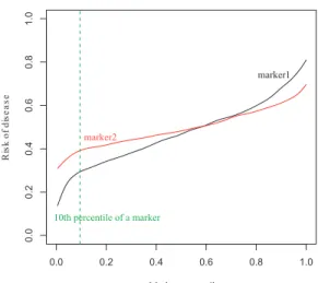
Figure 2: Biomarker 1 is more predictive than biomarker 2.
2.3.2 Predictiveness curve
Although ROC curve has been the most popular method for a biomarker evaluation, it does not take a risk distribution into account. Suppose all diseased subjects have same risk values of 0.52 and all non-diseased subjects have values of 0.51. In the ROC analysis, this would result in a perfect discrimination. Such a weakness triggers researchers to evaluate biomarkers from a different perspective. Huang et al. [21] published a predictiveness curve as a graphical way to present a predicted risk. It is a plot of predicted riskR(v) against thevth
percentile of the biomarker, where R(v) = P r[D= 1|Y =F−1(v)] and F is the cumulative distribution function of biomarker Y. Even though the original scales of the biomarkers are not comparable because the measurement can be different, they are transformed to a common scale in the predictiveness curve by using a percentile of the biomarker. It has been pointed out in many papers that the biomarker with a strong predictive capacity has steeper curves that corresponds to a wide variation in risk [21] [30] [31]. In Figure2, the biomarker 1 is more predictive than the biomarker 2 because more subjects are in high or low end of
the risk. For example, the subjects in the bottom 10% of the marker distribution have risks in the range of (0.15, 0.30) according to biomarker 1, but in a much higher range (0.30, 0.40) according to biomarker 2. If the predictiveness curve is close to the horizontal line, the biomarker is no more helpful for making a medical decision.
2.3.3 C-index
The C-index was proposed by Harrell et al. [32] as an overall measure of discrimination accuracy for survival outcome. The concept of C-index was motivated by Kendall’s τ, a nonparametric version of correlation. In their original paper, the C-index was applied not only to survival data but also to binary data. They pointed out that the C-index for binary outcome is equivalent to the AUC. The definition of AUC for binary outcome is the prob-ability that the diseased subject has worse biomarker value than the non-diseased subject. Changing the outcome from a binary to survival time, the C-index is defined as the prob-ability that the patient with better biomarker value will have a longer survival time than the patient with worse biomarker record, assuming that these two patients are selected at random.
Suppose that (Zi, Ui, Wi, Yi) are the actual survival time, predicted survival time,
predicted probability of survival at time t, and time-invariant biomarker measurements for ith subject (i = 1,· · ·, N), respectively. Harrell et al. [33] expressed C-index as P r(U
i <
Uj|Zi < Zj). In practice, it is hard to predict individual’s survival time. It is noted that
the predicted probability of survival until any fixed time point (Wi) can take place of the
predicted survival time(Ui), if two estimates have one-to-one correspondence. One advantage
in the application is that this relationship holds when the proportional hazard assumption is satisfied. Under the proportional hazard model, S(t|Yi) = (S0(t))β
tYi
, where S(t|Yi) is the
survival function given the biomarker value Yi, S0(t) is the baseline survival function andβ
is a regression parameter, theUi and Wi are exchangeable, because [34]
Wi < Wj ⇐⇒S(t|Yi)< S(t|Yj)⇐⇒ ∫ ∞ 0 S(t|Yi)dt < ∫ ∞ 0 S(t|Yj)dt⇐⇒ ∫ ∞ 0 t·f(t|Yi)dt < ∫ ∞ 0 t·f(t|Yj)dt ⇐⇒Ui < Uj.
Therefore, P r(Ui < Uj|Zi < Zj) = P r(Wi < Wj|Zi < Zj) = P r(βYi > βYj|Zi < Zj). The
C-index of 1 indicates that the model has a perfect discrimination power, whereas a value of 0.5 corresponds to an uninformative model.
Nonparametric version of estimation is possible for the C-index. A pair of subjects is said to be concordant if (βYi > βYj , Zi < Zj) or (βYi < βYj ,Zi > Zj). In contrast, a pair
(βYi > βYj ,Zi > Zj) or (βYi < βYj ,Zi < Zj) is said to be discordant. It is noted that not
all pairs are usable to determine concordance and discordance. A pair is usable only when one subject has an event before the other experiences an event or censored. For example, we discard pairs if neither of subjects have events or two individuals have the same survival time. Let R be a set of all usable pairs and Q be a total number of usable pairs in R. The C-index is estimated by ˆ C = 1 Q ∑ (i,j)∈R cij, where cij =
1 if (Zi < Zj and βYi > βYj) or (Zi > Zj and βYi < βYj)
0 if (Zi < Zj and βYi < βYj) or (Zi > Zj and βYi > βYj).
The original C-index is investigated further to overcome shortcomings. Yan and Greene [35] found that the C-index depends on the number of tied pairs. Therefore, in the presence of large proportion of tied pairs, they recommended to report both C-indices with and without ties. Another modification is done by Uno et al. [36] for censored survival data. To overcome the C-index’s dependence on the underlying censoring distribution, they presented the consistent estimates which is free of censoring by using an inverse probability weighting technique. The confidence interval for ˆC is developed by Pencina and D’Agostino [34]. The
100(1 - α)% confidence interval is ˆC±zα/2 √ d V ar( ˆC), d V ar( ˆC) = 4 N(pc+pd)4 (p2dpcc−2pcpdpcd+p2cpdd), pc = 1 N(N −1) ∑ i ci , pd = 1 N(N −1) ∑ i di pcc = 1 N(N −1)(N −2) ∑ i ci(ci−1) , pdd = 1 N(N −1)(N −2) ∑ i di(di−1) pcd = 1 N(N −1)(N −2) ∑ i cidi,
andci is the number of concordant pairs,di is the number of disconcordant pairs with theith
subject in the sample, andzα/2 is (1 - α/2) percentile of the standard normal distribution.
2.3.4 Time dependent ROC analysis
When a biomarker is used for a diagnosis of disease that changes over time, the original ROC analysis is no longer applicable. In the interval monitoring framework, DeLong et al. [37] and Parker and DeLong [38] developed the new ROC methodology using parameter estimates from discrete logistic regression. When continuous time to event data are available, however, time dependent ROC analysis could be performed. The time dependent ROC was introduced as an extension of the existing concept for sensitivity and specificity to survival outcome. We assume that the higher biomarker values are more indicative of shorter survival time. There are three different definitions of time dependent ROC.
A cumulative/dynamic time dependent ROC is used when the main question is whether the biomarker can distinguish the patients who have experienced the event by time t and who have not [39]. The cumulative case refers to the subject who has experienced the event during the time interval (0, t], whereas the dynamic control refers to the subject with no event by time t. With the cutoff point ofc, sensitivity and specificity are defined as
Sensitivity(t) =P r(Y > c|Z ≤t) Specif icity(t) = P r(Y ≤c|Z > t).
The time dependent sensitivity and specificity are estimated using Kaplan-Meier estima-tor based on the subset of Y ≥ c or weighted Kaplan-Meier estimator based on nearest neighbor kernel. The confidence interval of time dependent ROC curve is calculated by bootstrap method. This ROC method can be used clinically when the sensitivity of stan-dard and new diagnostic measures are compared at certain time points to check whether the new measure provides improved discrimination during the follow-up time. Later, the cumulative/dynamic time dependent ROC is generalized to longitudinal biomarker [40] and competing risk outcomes [41]. For the longitudinal biomarker, the question of interest is how well a biomarker measured at a certain time point after the baseline can discriminate diseased and non-diseased subjects in a subsequent time interval.
Alternative approach is an incident case and dynamic control time dependent ROC [42]. Under this definition, only subject who has an event at time t plays a role of case. The dynamic control corresponds to the subject who is event free by timet. The incident/dynamic time dependent sensitivity and specificity are defined as
Sensitivity(t) = P r(Y > c|Z =t) Specif icity(t) = P r(Y ≤c|Z > t).
The sensitivity can be estimated under proportional hazard model by computing the ex-pected fraction of failures with a biomarker level greater thanc. The specificity is estimated by the empirical distribution function for biomarker among those who survive beyond t. Bootstrap confidence interval can be constructed for nonparametric time dependent ROC. It is particularly useful when investigators want to display the incident discrimination ability over time. It is interesting to know that the C-index is a weighted average of the area under the incident/dynamic time dependent ROC [42].
The last version of time dependent ROC is defined with respect to incident case and static control [43] [44]. Defining the case as the subject who experiences an event at time t, the control is the subject who has not developed an event until a fixed time point at t♯.
only on the case group. The sensitivity and specificity is given as
Sensitivity(t) = P r(Y > c|Z =t) Specif icity(t) = P r(Y ≤c|Z > t♯).
Zheng and Heagerty [45] estimated the incident/static time-dependent ROC curve by model-ing the biomarker distribution conditional on the event status in a semiparametric way. The ROC curve was expressed as a function of location and scale parameters from the biomarker distribution. Incident/static ROC method is useful in a retrospective study especially when the time to event is certain. As an alternative estimation method, the direct regression approach of ROC curve was comprehensively reviewed and extended by Cai et al. [46] and Pepe et al. [47]. Confidence interval of the ROC curve can be based on bootstrap samples or asymptotic property under certain regularity condition.
In this dissertation, we focus on the cumulative/dynamic time dependent ROC. One of the questions addressed from our study is how well a biomarker can discriminate subjects who had an event until time pointtand those who remained event free up tot. To measure a biomarker’s discrimination potential for cumulative events by timet, which are time depen-dent measures, cumulative/dynamic time dependepen-dent ROC analysis may be more appropriate than others.
3.0 DISCRIMINANT ANALYSIS FOR CENSORED LONGITUDINAL BIOMARKER DATA
Discriminant analysis is commonly used to evaluate the ability of candidate biomarkers to separate patients into pre-defined groups. Extension of discriminant analysis to longitudinal data enables us to improve the classification accuracy based on biomarker profiles rather than on a single biomarker measurement. However, the biomarker measurement is often limited by the sensitivity of the given assay, resulting in data that are censored either at the lower or upper limit of detection. We develop a discriminant analysis method for cen-sored longitudinal biomarker data based on mixed models. The biomarker performance is assessed by AUC. Through the simulation study, we show that our method is better than the simple substitution methods in terms of parameter estimation and evaluating biomarker performance. We apply our method to a biomarker study aiming to identify biomarkers that are predictive of the recovery from acute kidney injury for patients on renal replacement therapy.
3.1 INTRODUCTION
As a noninvasive and cost-effective tool for diagnosis and prognosis of acute and chronic diseases, biomarkers have received increasing attention for many decades. Two questions raised commonly in the biomarker studies are (1) how to classify subjects into disease and non-disease groups based on their measurements and (2) how to evaluate the clinical utility of the biomarker. For classification and evaluation, several methods such as logistic re-gression, discriminant analysis, and ROC curve have been widely applied for cross-sectional
data. However, more and more studies highlight the importance of the temporal change of biomarkers which can provide better understanding of the development of a disease [48]. Longitudinal biomarkers have been shown to lead to more accurate diagnosis than single measurement. For example, de Leon et al. [49] stated that the diagnostic accuracy of mild cognitive impairment is improved when longitudinal cerebrospinal fluid marker is used. If biomarkers are measured repeatedly over several time points, we may need specialized tech-niques for capturing important time-related patterns in the repeated measurements. The other concern in the biomarker study is the LOD. If an instrument is not sensitive enough to detect very high and low concentrations, only measurements which lie between lower and upper detection limits are observable. The results from inappropriate handling of these types of data may mislead physicians in medical decision making.
Our work is motivated from the Biological Markers of Recovery for the Kidney (BioMaRK) study. The recovery of a kidney function following the acute kidney injury (AKI) is an im-portant determinant of morbidity and may have long-term implications for the health and well-being of patients [50]. Hence, identifying informative biomarkers for predicting a 60-day recovery is one of the primary goals of this study. There has been much effort in the biomarker discovery related to AKI due to its unacceptably high mortality rates. Most stud-ies focus on evaluating biomarker performance based on a single measurement. Even when the biomarkers are measured over time, it is common to analyze the biomarker at each time point separately or choose arbitrarily a summary measure such as change score or slope to incorporate the longitudinal information. However, investigators are often more interested in the overall performance of the longitudinal biomarker because biomarker evolution can reveal better the biological process of a disease. In the BioMaRK study, multiple urinary biomarkers are longitudinally measured, and the measurements of some biomarkers are cen-sored due to detection limits. The objective of our research is to develop a classification method for the longitudinal biomarkers subject to left or right censoring due to lower or upper detection limit.
We develop the new classification and evaluation methods to take both censoring and repeated measures into account. Discriminant analysis has been extended to the longitudinal setting with a discriminant function estimated from mixed models [51] [52] [53] [54]. Further
generalization to multivariate longitudinal data has been discussed by Marshall et al. [55] using multivariate nonlinear mixed models. Kohlmann et al. [56] introduced the longitudinal quadratic discriminant analysis and evaluated the classification performance using the ROC curve and Brier score. If longitudinal data are censored due to a detection limit, however, earlier proposed methods cannot produce an expected result. The problem of left-censoring has been studied by many researchers [4] [19] [18]. They considered maximum likelihood approaches to incorporate the censoring issue. As a related work to our objective from a discriminant analysis perspective, Langdon et al. [57] discussed how to classify subjects based on two censored variables. They estimated parameters by maximizing the marginal likelihood function of bivariate normal distribution. These estimates were plugged into the classifier formed by Bayes optimum decision rule. We extend the idea of Langdon et al. [57] to develop classification methods for longitudinal censored data, and show how AUC can be constructed from discriminant analysis.
The organization of this chapter is as follows. In section3.2, we introduce the underlying theory of our discriminant analysis method. We describe how to classify subjects and how to evaluate biomarker performance in the presence of censoring. In section 3.3, we compare our method with simple substitution methods using simulated data. Finally, our method is applied to the BioMaRK study to predict a patient’s recovery status from AKI within 60 days after the enrollment.
3.2 METHOD
3.2.1 Linear mixed model for biomarker data
High dimensionality, serial correlations, unbalanced or unequally spaced repeated measures, and missing data are typical issues that people encounter in the longitudinal analysis. Mixed model is one of the popular approach to handle these problems [58]. The linear mixed model captures the correlations between repeated measurements within a subject via random effects (also called subject specific effects). Also, it can accommodate missing data when the missing
and measurement processes are independent (missing completely at random; MCAR), or the missing process depends only on the observed measurements (missing at random; MAR). Let Yij be the biomarker measurement on theith individual at the jth time point, (i= 1,· · ·,N;
j = 1,· · ·,ni). Thus,Yi = (Yi1,· · · , Yini)tis anni×1 vector of measurements corresponding
to theith subject. The linear mixed model relatingY
i to a set of covariates can be expressed
in the matrix notation as
Yi =Xiβ+Ziγi+ei,
whereXi is anni×pdesign matrix of fixed effect,β is ap×1 population parameter vector,
andZi is an ni×q design matrix of random effect. Random errorei and random effectγi are
independent and normally distributed with ei ∼N(0, Ri) and γi ∼N(0, Gi). Marginally, Yi
is normally distributed with mean Xiβ and covariance matrix Σi =ZiGiZit+Ri.
Parameters in the linear mixed model can be estimated from the likelihood function formulated given the random effects. A likelihood function is simplified based on the mixed model assumption that longitudinal observations are independent given the random effects. To handle the censoring of biomarker measurements, we use the method similar to Lyles et al. [19]. Suppose lower detection limit and upper detection limit are τlo and τup,
respec-tively. The likelihood function is constructed using the normal density functionf(Yij|γi) for
observed measurements and the cumulative distribution function F(τlo|γi) or 1−F(τup|γi)
for censored parts. Let θ denote the vector of parameters in the covariance matrices. The final likelihood function for the covariance parameter vector θ and coefficient vector β is given by L(β, θ;Y) = N ∏ i=1 [∫ Rq ni ∏ j=1
{f(Yij|γi)I(dij=0)F(τlo|γi)I(dij=1)(1−F(τup|γi))I(dij=2)}f(γi)dγi
] , dij = 0 if Yij is completely observed 1 if Yij is left censored at τlo 2 if Yij is right censored at τup, I(·) is an indicator function.
Once the likelihood function is defined depending on the censoring types, set of param-eters θ and β are estimated by maximizing the likelihood function. Because the likelihood function includes cumulative distribution function to account for censored biomarker, we apply SAS procedure Proc nlmixed to obtain the estimates. The Proc nlmixed proce-dure allows us to specify the general form of distribution given the random effects. Integral approximation is done by an adaptive Gaussian quadrature method and the likelihood is maximized by dual quasi-Newton algorithm [59].
3.2.2 Discriminant analysis
We adopt the concept of discriminant analysis to construct the classifier using longitudinal censored biomarker measurements. Discriminant analysis arises from the desire to use an optimal classification rule, and it is often based on the assumption of normal distribution for two separate groups. Let fk(y) denote the normal density function (with mean µk and
variance matrix Σk) of the longitudinal biomarker measurements for the subjects in groupk
(k = 0, 1). For a subject with biomarker dataY, the posterior probability of assigning the subject into groupk is given by
P r(Groupk|Y) =
fk(Y)πk
f0(Y)π0+f1(Y)π1
,
where πk is the prior probability that a subject belongs to group k without the knowledge
of Y. The ratio P r(Group1|Y)/P r(Group0|Y) is then used as a discriminant function and
compared with a pre-defined cutoff point to determine the group membership. Noting that the corresponding log ratio
logP r(Group1|Y) P r(Group0|Y) =logf1(Y) f0(Y) +logπ1 π0,
we refer to the first term as a risk score S =log(f1(Y)/f0(Y)).When two groups have same
variance matrix (i.e. Σ0 = Σ1 = Σ), the risk score is simplified as
S = { Y − 1 2(µ 1 +µ0) }t Σ−1(µ1−µ0). (3.1)
When variance matrices for two groups have different forms (i.e. Σ0 ̸= Σ1), the risk score is S = Y t(Σ 0−1−Σ1−1 ) Y 2 +Y t( Σ1−1µ1−Σ0−1µ0 ) − log|Σ1|/|Σ0| 2 −1 2 ( µ1tΣ1−1µ1−µ0tΣ0−1µ0 ) .
The distributional parameters can be estimated from the mixed model. The estimation ofS for each individual depends on whether the subject has censored measurement or not. When Y is completely observed, the risk score S can be directly calculated from equation (3.2.2) usingY. If some components ofY are censored, we will substitutefk(Y) in equation (3.2.2)
byfk∗(Y), defined as fk∗(Y) = ∫ Rq ni ∏ j=1
{fk(Yij|γi)I(dij=0)Fk(τlo|γi)I(dij=1)(1−Fk(τup|γi))I(dij=2)}fk(γi)dγi
A new patient is classified by comparing his/her risk score to a pre-selected threshold. For example, if we use the cutoff point driven by the decision theory with Bayes 0-1 loss function, the subject is classified into group 1 if ˆS > 0, and classified into group 0, otherwise.
3.2.3 Evaluation of classification performance
AUC has long been defined for cross-sectional test results. Suppose variables T0 and T1 are the test results from normal and disease groups. The AUC is defined as P r(T1 > T0),
that is, a probability that the test result for a randomly chosen individual with a disease is more indicative of that disease than the test result from a normal subject. The test result can be a continuous biomarker measurement. When the biomarker is measured over time, the test result is a multivariate measure. To summarize the classification performance of a multivariate test result to a univariate measure, we use the risk score S to serve as a test result in the AUC calculation. In the following, we show how non-parametric and parametric estimates of AUC are calculated based on the risk score S.
With risk score S used as a test result, we may define S1 and S0 as the risk scores for
a randomly chosen subject from group 1 and group 0 respectively. Suppose there are n0
controls and n1 cases in the data set. The sensitivity and specificity based on the estimated
risk score ˆS can be formulated as
1−Specif icity = 1 n0 n0 ∑ i=1 I ( ˆ S0 i > c ) Sensitivity = 1 n1 n1 ∑ j=1 I ( ˆ S1 j > c ) ,
for a threshold c. The empirical ROC curve is obtained by connecting points [sensitivity(c), 1-specificity(c)]. The posterior probabilitiesP r(Groupk|Y) have also been used to construct
the empirical ROC curve [52] [55] [56] in the longitudinal discriminant analysis. Note that the posterior probability of belonging to group 1 isP r(Group1|Y) =eS / (eS + 1), which is a
monotone transformation of S. Thus these two approaches lead to the same AUC given the invariant property of ROC curve under monotone transformations. We can use trapezoids method to estimate AUC and the method by DeLong et al. [25] for variance estimation. In the presence of censoring, empirical AUC tends to produce lower values because it reflects the actual discrimination ability of incomplete information rather than a potential discrimi-nation ability which could be achieved if LOD is eliminated.
Parametric estimation of AUC
In a special case when two groups have a common covariance matrix, the risk score has a linear form in terms of Y (3.1). Then the AUC can be estimated based on the distribu-tional assumption of the longitudinal biomarker measurements. A smooth ROC curve can be obtained by Sensitivity= Φ ( λt(µ1−µ0) √ λtΣλ + Φ −1(1−Specif icity) ) , with λ= Σ−1(µ1−µ0),
and the AUC is defined as AU C =P r[S1 > S0] =P r [{ Y1−1 2(µ 1 +µ0) }t Σ−1(µ1 −µ0)> { Y0− 1 2(µ 1+µ0) }t Σ−1(µ1−µ0) ] =P r[{Σ−1(µ1−µ0)}tY1 >{Σ−1(µ1−µ0)}tY0 ] = Φ ( λt(µ1−µ0) √ λt(2Σ)λ ) , (3.2)
where Φ is a standard normal cumulative distribution function. The ROC curve and AUC are estimated using ˆµ0, ˆµ1 and ˆΣ from the linear mixed model. Because the AUC is entirely
determined by parameters µ1, µ0, and Σ, it remains intact unless the estimates ˆµ1, ˆµ0, ˆΣ
are biased by the censored data. The standard error of AUC estimate can be calculated following McClish’s method [60].
3.3 SIMULATION STUDY
We conduct simulation study to evaluate the performance of the proposed discrimination method. In practice, substitution methods are often used to handle the censored data due to detection limits. Usually the censored observations are replaced by LOD or LOD/2. We investigate how the discrimination measure AUC is affected by the censoring problem and under what scenarios the naive substitution methods tend to introduce significant bias. We also examine the impact of misspecification of covariance structure on the discrimination evaluation of longitudinal biomarker profile. In the simulation, we use the same set of sub-jects in the estimation of parameters and AUC, which tends to make classification accuracy overoptimistic. However, the bias of AUC due to this will be negligible for considered sample size and number of parameters.
We generate longitudinal biomarker measurement Yij for the subject iat time point Tij
from the mixed model:
Yij =φ1+φ2Xi+φ3Tij +φ4(Xi×Tij) +ai+biTij +eij, (3.3) where eij ∼N(0, σ2) and ai bi ∼N 0 0 , σ2a σab σab σ2b .
Xi is a dichotomous variable, indicating the group membership (0 or 1) and Tij is a time
factor, indicating the follow up times of measurements (Tij = 1,2,3,4). Random intercept ai
and random slopebi are included in the model to reflect the deviation of the subject specific
trajectory from the population trajectory. We assume that random effects are independent of the random error. Note that the classification performance of a biomarker is determined by the underlying separability in biomarker measurements between groups. The separability not only depends on the regression coefficient parameters which specify the difference in mean, but also the parameters in the covariance matrix. Larger variability in Y makes it more difficult to divide the two groups. We fix the regression parameters at φ1 = 1.0,φ2 = φ3 =
0.5,φ4 = -1.0, and the covariance parameters atσ2 = 1.0,σab = 0.0. This corresponds to the
scenario where the trajectories of two groups start at different baseline levels and increase over time for one group and decrease for another group. Moreover, the variabilities of biomarker measurements increase over time. To simulate biomarker data with different discrimination ability, we change the variance inY through the variance parameters of random effects, i.e., σ2
a = σ2b = 0.5, 1.0, and 2.0 with higher values representing poor separation between two
groups. We choose lower detection limitτlo empirically so that the censoring rate of 20% and
40% can be achieved. We simulate 100 datasets, each including 200 subjects from individual group.
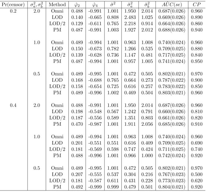
The parameter estimates from the linear mixed model as well as parametric estimates of AUCs, associated standard errors (se) and empirical 95% coverage probabilities (CP) are summarized in Table 2. Comparing to the omniscient estimates based on the uncensored complete data, the parameter estimates of the group (φ2) and interaction (φ4) effects are
Table 2: Parametric estimation of AUC: Comparison of the discriminant ability between proposed method (PM) and substitution methods (φ2 = 0.5, φ4 = -1.0, σ2 = 1.0)
Pr(censor) σa2, σ2b Method φˆ2 φˆ4 σˆ2 σˆa2 σˆ2b AU Cˆ (se) CP 0.2 2.0 Omni 0.488 -0.991 1.001 1.950 2.014 0.687(0.026) 0.960 LOD 0.140 -0.665 0.808 2.483 1.025 0.669(0.026) 0.890 LOD/2 0.129 -0.611 0.765 2.218 0.914 0.664(0.026) 0.860 PM 0.487 -0.991 1.003 1.927 2.012 0.688(0.026) 0.940 1.0 Omni 0.489 -0.994 1.001 0.963 1.008 0.740(0.024) 0.960 LOD 0.150 -0.673 0.782 1.266 0.525 0.709(0.025) 0.880 LOD/2 0.139 -0.628 0.736 1.147 0.481 0.717(0.025) 0.840 PM 0.487 -0.994 1.001 0.957 1.005 0.741(0.024) 0.950 0.5 Omni 0.489 -0.995 1.001 0.472 0.505 0.802(0.021) 0.970 LOD 0.168 -0.688 0.765 0.664 0.273 0.787(0.022) 0.900 LOD/2 0.158 -0.654 0.725 0.616 0.257 0.783(0.022) 0.850 PM 0.489 -0.996 1.002 0.469 0.504 0.803(0.021) 0.960 0.4 2.0 Omni 0.488 -0.991 1.001 1.950 2.014 0.687(0.026) 0.960 LOD 0.198 -0.548 0.567 1.242 0.791 0.660(0.026) 0.810 LOD/2 0.187 -0.556 0.589 1.351 0.803 0.661(0.026) 0.820 PM 0.470 -0.987 1.001 1.911 2.056 0.685(0.026) 0.910 1.0 Omni 0.489 -0.994 1.001 0.963 1.008 0.740(0.024) 0.960 LOD 0.201 -0.551 0.551 0.616 0.409 0.709(0.025) 0.690 LOD/2 0.181 -0.569 0.598 0.747 0.424 0.711(0.025) 0.740 PM 0.488 -0.996 1.001 0.966 1.000 0.742(0.024) 0.920 0.5 Omni 0.489 -0.995 1.001 0.472 0.505 0.802(0.021) 0.970 LOD 0.207 -0.555 0.537 0.304 0.216 0.767(0.023) 0.500 LOD/2 0.181 -0.587 0.611 0.431 0.228 0.773(0.023) 0.620 PM 0.492 -0.999 0.999 0.479 0.501 0.804(0.021) 0.920
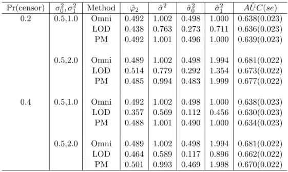
Table 3: Nonparametric estimation of AUC: Comparison of the discriminant ability between proposed method (PM) and substitution methods (φ2 = 0.5, σ2 = 1.0)
Pr(censor) σ02, σ21 Method φˆ2 ˆσ2 σˆ02 σˆ12 AU Cˆ (se) 0.2 0.5,1.0 Omni 0.492 1.002 0.498 1.000 0.638(0.023) LOD 0.438 0.763 0.273 0.711 0.636(0.023) PM 0.492 1.001 0.496 1.000 0.639(0.023) 0.5,2.0 Omni 0.489 1.002 0.498 1.994 0.681(0.022) LOD 0.514 0.779 0.292 1.354 0.673(0.022) PM 0.485 0.994 0.483 1.999 0.677(0.022) 0.4 0.5,1.0 Omni 0.492 1.002 0.498 1.000 0.638(0.023) LOD 0.357 0.569 0.112 0.456 0.630(0.023) PM 0.488 1.001 0.490 1.000 0.634(0.023) 0.5,2.0 Omni 0.489 1.002 0.498 1.994 0.681(0.022) LOD 0.464 0.589 0.117 0.896 0.662(0.022) PM 0.501 0.993 0.469 1.998 0.670(0.022)
heavily biased when the censored observations are replaced by LOD or LOD/2. The pro-posed method (PM) provides approximately unbiased estimates. As expected, the bias of estimates continuously acts on the discriminant analysis and attenuates the AUC. Substi-tution methods provide increasingly smaller AUCs with poor coverage probabilities as the censoring proportion is increased. Our method, however, presents comparable AUCs to the omniscient values, and the coverage probabilities are close to the nominal level of 0.95.
Generalizing the assumption on the variance matrix, we also estimate the AUC empiri-cally as described in section 3.2.3. We make the variance matrices for two groups different by allowing two random effects in the linear mixed model:
Yij =φ1+φ2Xi+φ3Tij +a0i+a1i+eij,
where eij ∼ N(0, σ2), a0i ∼ N(0, σ20) and a1i ∼ N(0, σ12). Two random intercepts a0i, a1i
and error eij are assumed to be independent each other. The parameters are fixed at φ1
= φ3 = 1.0, φ2 = 0.5, σ2 = 1.0, and (σ02, σ12) = (0.5, 1.0), (0.5, 2.0). Individual group
Table 4: Performance measures and fit statistics from different models
Pr(censor) σ2a, σb2 Model AIC BIC AUC(se)
0.2 2.0 True 0.687 RI 6604.35 6628.30 0.782(0.022) RS 5686.15 5710.10 0.683(0.026) RI + RS 5599.84 5631.77 0.688(0.026) 1.0 True 0.741 RI 5991.66 6015.61 0.844(0.019) RS 5347.83 5371.77 0.732(0.024) RI + RS 5312.57 5344.50 0.741(0.024) 0.5 True 0.803 RI 5492.32 5516.27 0.898(0.015) RS 5083.71 5107.66 0.794(0.022) RI + RS 5070.54 5102.47 0.803(0.021) 0.4 2.0 True 0.687 RI 5236.54 5260.49 0.772(0.023) RS 4630.07 4654.02 0.689(0.026) RI + RS 4568.18 4600.10 0.685(0.026) 1.0 True 0.741 RI 4836.06 4860.01 0.829(0.020) RS 4401.94 4425.89 0.736(0.024) RI + RS 4376.95 4408.88 0.742(0.024) 0.5 True 0.803 RI 4513.40 4537.35 0.884(0.016) RS 4228.21 4252.16 0.797(0.022) RI + RS 4219.54 4251.47 0.804(0.021)
the result averaged over 100 datasets. Unlike the parametric estimate of AUC, the empirical AUC estimate tends to be smaller than a potential AUC because the nonparametric ROC curve is constructed based on the individual’s score. If the individual has censored data for at least one time point, his/her score is affected by incomplete measurements and its original discriminative potential is reduced. In contrast, the parametric AUC is close to the omniscient estimate which reflects the potential discrimination ability, because it does not depend on the individual’s score, but depends on the mean and variance for each group.
To examine the impact of model misspecification on the biomarker evaluation, we gen-erate the data from model (3.3), which is referred to as random intercept and slope (RI + RS) model, but fit the data with three different models: RI + RS model, random intercept (RI) only model, and random slope (RS) only model. Table 4 shows the AUC estimates, associated standard errors, and goodness-of-fit statistics, Akaike information criterion (AIC) and Bayesian information criterion (BIC), from three mixed models. Both RI only and RS only models yield biased AUC estimates. The RI model overestimates the AUC, while the RS model underestimates the AUC. Only the correct RI + RS model produces AUC estimate close to the true one. In practice when we rarely know the true model, how can we believe that we have a correct performance measure? It appears that the goodness of fit statistics such as AIC and BIC can be used as a general guideline. Overall, the model with better goodness of fit (smaller AIC and BIC) produces AUC estimate closer to the true one. Our results are consistent with what was pointed out by Kohlmann et al. [56], incorrect model specification may lead to spuriously better or worse performance measures.
3.4 APPLICATION TO BIOMARK STUDY
The Biological Markers of Recovery for the Kidney (BioMaRK) is an observational study conducted as an ancillary study of the NIDDK-funded Acute Renal Failure Trial Network (ATN) study. ATN study is a multicenter, prospective trial of two strategies for renal re-placement therapy in critically ill patients with acute kidney injury (AKI) [61]. One of the primary goals of the BioMaRK study is to find biomarkers predictive for the recovery
1 7 14 4 5 6 7 8 9 NGAL: No recover 1 7 14 NGAL: Recover 1 7 14 6 7 8 9 0 1 1 1 2 1 1 7 14 HA: Recover Log(NGAL) HA: No recover
Days after enrollment
Log(HA)
Figure 3: Boxplots of the log transformed NGAL and HA by recovery status
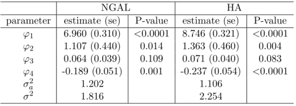
of renal function by 60 days after enrollment. The ’Recover’ is defined as a survival with dialysis-independent renal function, and ’No-recover’ indicates a death or dependence on dialysis. Serial measurements of plasma and urinary biomarkers are collected from the ATN study participants who signed the consent form for biomarker determination. For illustration purpose, we focus on the analysis of two urinary markers, Neutrophil Gelatinase-Associated Lipocalin (NGAL) and Hyaluronic Acid (HA), that are obtained for 76 patients at day 1, 7, and 14 after enrollment. Among 76 subjects, 38 (50%) recovered from AKI. NGAL is one of the widely used urinary biomarkers for prediction of AKI. HA is a new biomarker that is recently reported to correlate with both proteinuria and renal function in progressive renal disease. NGAL measurements are censored by two upper detection limits at 500 and 10000 ng/mg.Cr. The proportions of censoring at day 1, 7 and 14 are 25.4%, 34.0%, and 27.3%, respectively. HA level over 2029931.3 ng/mg.Cr is not measurable due to the detection limit. Most of HA levels are within the detection limit and only 2.7% are censored at day 1. We take a log transformation for NGAL and HA measurements to normalize the distribution.
Figure3presents the group-level boxplots of NGAL and HA on a log scale over three time points, where the censored observations are replaced with the detection limit. It appears that both HA and NGAL levels go up a little at day 7 for the non-recovery group, but go down over time for the recovery group. We consider several candidate models of different covariance matrices (RI only, RS only, and RI + RS model) and different form of group-specific trajectories. We choose the final model with the smallest AIC and BIC as follows.
Yij =φ1+φ2Recoveri+φ3T imeij +φ4Recoveri×T imeij +ai+eij
where eij ∼N(0, σ2) , ai ∼N(0, σa2) Recoveri =
0 if subject i didn’t recover within 60 days 1 if subject i recovered within 60 days
The parameter estimates are shown in Table 5. The HA level correlates with the group membership a little stronger than the NGAL does, as indicated by the magnitude and significance of the group effect and group by time interaction effect. It gives an evidence that HA may have better discriminant ability than NGAL. The parametric AUC estimate (standard error) for NGAL is 0.822 (0.047), and for HA is 0.853 (0.043) (Figure 4 left: the black solid line and blue dotted line is for NGAL and HA, respectively). Substitution method using LOD/2 produces AUC estimates of 0.612 (0.063) for NGAL and 0.841 (0.040) for HA. We also perform cross sectional analysis to examine the discrimination ability of single biomarker measurement. The AUCs for NGAL day 1, day 7, and day 14 measurements are 0.662, 0.519, and 0.729 respectively. The corresponding AUCs for HA are 0.659, 0.563, and 0.849. Clearly, the discrimination performance is significantly improved by using the biomarker profile rather than the measurement on a single day.
To assess the prediction capacity of the biomarkers, we take the risk distribution into account using a predictiveness curve presented by Huang et al. [21]. Predictiveness curve is