Parallel Support Vector Machines
Dominik Brugger
WSI-2006-01
ISSN 0946-3851
Dominik Brugger
Arbeitsbereich Technische Informatik
Sand 13, 72074 T¨ubingen
[email protected]
c
Parallel Support Vector Machines
Dominik Brugger
Arbeitsbereich Technische Informatik Eberhard-Karls Universit¨at T¨ubingen
Sand 13, 72074 T¨ubingen
Abstract
The Support Vector Machine (SVM) is a supervised algorithm for the solution of classification and regression problems. SVMs have gained widespread use in recent years because of successful applications like character recognition and the profound theoretical underpinnings con-cerning generalization performance. Yet, one of the remaining draw-backs of the SVM algorithm is its high computational demands during the training and testing phase. This article describes how to efficiently parallelize SVM training in order to cut down execution times. The par-allelization technique employed is based on a decomposition approach, where the inner quadratic program (QP) is solved using Sequential Min-imal Optimization (SMO). Thus all types of SVM formulations can be
solved in parallel, includingC-SVC andν-SVC for classification as well
asε-SVR andν-SVR for regression. Practical results show, that on most
problems linear or even superlinear speedups can be attained.
1
Introduction
The underlying idea of supervised algorithms is learning by examples. Thus given a set
xi∈ Xof input data and associated labelsyi∈ Ythe algorithms learns a mapping
f : X 7→ Y using the training data given. If the algorithm generalizes well, then the
number of correctly classified inputs on unknown test data will be high in the classification case. Analogously for regression the mean squared error (MSE) will be low.
Support Vector Machines (SVM) are a supervised algorithm first introduced in [21]. One of its advantages over other supervised algorithms, is the possibility to derive bounds concern-ing the generalization performance on unseen test data after the trainconcern-ing phase. Another nice property of SVMs concerns the incorporation of prior knowledge about a learning
problem, which can be achieved by a kernel function [14]. The kernel functionk(xi, xj)
computes the dot product between input patternsxiandxjthat have been mapped into a
higher dimensional, or even infinite dimensional feature space using a mappingΦ:
k(xi, xj) =hΦ(xi),Φ(xj)i.
Since the kernel function just evaluates the dot product between the mapped patterns the mapping is not carried out explicitly. By substitution of dot products with a kernel function, the SVM constructs a separating hyperplane with maximum margin in the feature space and this separating hyperplane then corresponds to a nonlinear decision surface in input space. Different kernel functions have been suggested for a wide range of applications, including string kernels for document classification, spike kernels for neuronal signal processing and graph kernels for bioinformatics [14],[16],[10]. Although this clean concept of separation
between prior knowledge and learning algorithms has been adopted quickly by many prac-titioners, the use of complicated kernel functions slows down SVM training considerably. One technique for avoiding this problem is the caching of kernel function evaluations first proposed in [11]. But as kernel functions will get more complex in future this might not be sufficient to speed up SVM training. One possible remedy for this problem is the parallel evaluation and caching of kernel function values as shown in [23, 22].
Another motivation for parallel SVM training are growing dataset sizes in many application areas, which usually range from several hundred thousand to millions of input patterns. Recent studies have shown, that subsampling the dataset in order to cut down training time is not an option in many cases, as it leads to a decrease in classification performance on the test set [17].
According to Moore’s law one might argue that many large scale problems which cannot be solved on single processor hardware today might be solvable tomorrow. But this statement is only true in part, if one takes a closer look at hardware developments in the last two years. Most of the acceleration is achieved at the moment by an emerging new architectural concept: the multicore architecture. Yet exploiting the performance of multicore processors requires new threaded or parallel software [2].
1.1 Related Work
Speeding up SVM training has been an issue that was addressed by many authors in the past. But most of the approaches are based on different formulations of the original SVM algorithm or they rely on approximation techniques.
The Core Vector Machine (CVM) can be applied to solve SVM classification and regression problems efficiently on large datasets [17, 18]. It relies on an approximation technique for computing minimum enclosing balls by a concept called coresets which has its originates from the field of computational geometry [3]. In contrast to the original SVM formulation the dual quadratic program (QP) to be solved is simplified, by penalizing margin errors
using the L2 loss function and additionally penalizing the hyperplane offsetb. This leads
to a QP problem with one simple linear constraint and a positivity constraint for the dual
variablesαwhich can be solved by the minimum enclosing ball algorithm.
An earlier approach which exploits the same kind of QP problem simplification is the La-grangian Support Vector Machine (LSVM) of [12]. The LSVM is very efficient for the
linear kernel and large problems in low dimensions (< 22), since it uses the
Sherman-Morrison-Woodbury identity [8] to invert the kernel matrix.
Parallelizing the original SVM formulation with L1 loss function for margin errors is done by the Cascade SVM [9]. It is based on the idea, that only a small number of the patterns in the training data set will end up as support vectors. Therefore the Cascade SVM splits the dataset into smaller problems and filters out support vectors in a cascade of SVMs which can work in parallel. Although there is a formal proof of convergence for the method, one remaining drawback is the size of the final problem to be solved which is dependent on the number of support vectors. Especially for noisy training data this final problem might be huge.
A different parallel technique for solving SVM problems is the parallelization of the de-composition approach first described in [11]. Recently is has been shown [23], that with appropriate working set selection and inner QP solver, this decomposition approach can gain impressive speedups in practice. However so far this approach has only be used for
the training ofC-SVC.
In the work described in this article the main focus is on solving the original SVM formu-lation of [21] in parallel. The adopted approach is the parallel decomposition technique introduced by [23]. This article studies several different inner solvers including SMO, a parallel version of an interior point code (LOQO) and the projected gradient method of [5]. It turns out, that in practice only SMO in combination with the decomposition technique is
able to solve all of the SVM formulations includingC-SVC,ν-SVC,ε-SVR andν-SVR
1.2 Outline
This article is organized as follows: Section 2 gives a brief introduction to the SVM algo-rithm and subsequently derives the underlying general form of the QP problem to be solved for the different SVM formulations. How these QP problems can be solved in practice is described in section 3. The decomposition method for large scale SVM training as well as details on the working set selection strategy and stopping criteria are described in section 4. Some hints on implementation specific details are given in section 5. Finally section 6 gives performance results on several large scale datasets.
2
Support Vector Machines
In the case of Support Vector Classification (SVC) labeled training data(xi, yi) ∈ X ×
Y, i= 1, . . . , mis given and the goal of the SVC algorithm is to learn a function
f :X 7→ Y, which can be subsequently used for the prediction of class labels on unknown
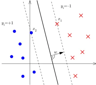
test data. Figure 1 shows a simple binary classification problem, where the two classes are
represented by balls and crosses. The SVC algorithm constructs a hyperplanehw, xi+b=
0with normal vectorwand offsetbto separate these two classes. Since there are many
possibilities for the location of this hyperplane, SVC searches for a hyperplane with the largest margin, where the margin is defined to be the distance of the closest point to the hyperplane. Intuitively this approach leads to a good solution with respect to the unknown test data, since classes are somewhat well separated. Indeed the choice of a large margin can be directly related to the generalization performance of the classifier in a formal way [14].
2 x 1 x =+1 i y ={1 i y w
Figure 1:Toy example of a binary classification problem where the points marked
by balls and crosses represent the two classes. The SVC algorithm maximizes the margin between the two classes, which is the distance between the two pointsx1
andx2 closest to the separating hyperplane. This distance can be expressed in
terms of the hyperplane normal vectorwand is equal to1/kwk.
The margin is exactly1/kwk, if the condition|hw, xii+b|= 1is satisfied by rescalingw
andbappropriately, since:
hw, x1i+b= +1, hw, x2i+b=−1
⇒ hw, x1−x2i= 2 ⇒ hw/kwk, x1−x2i= 2/kwk.
optimization problem: min w,b 1 2kwk 2 (1) subject to yi(hw, xii+b)≥1, ∀i= 1, . . . , m . (2)
If it is impossible to separate the data by a hyperplane, as often is the case in practice, a so
called soft margin hyperplane [14] can be computed by introducing slack variablesξi≥0
and relaxing (2). As a consequence the margin may be violated by some of the input
patternsxi, for whichξ >0. To nevertheless find a good classifier the number of violators
is restricted by penalizing the margin error with an L1 loss in the objective function leading to the following optimization problem:
min w,b,ξ 1 2kwk 2+C m X i=1 ξi (3) subject to yi(hw, xii+b)≥1−ξi, ∀i= 1, . . . , m . (4)
The parameterCtrades off between the number of margin errors and the size of the margin
and thus the generalization performance of the classifier. The optimization problem above is usually solved in its dual form which is obtained by incorporating equation (4) into the objective function (3) using the Lagrange function:
L(w, b, ξ, α, β) =1 2kwk 2+C m X i=1 ξi− m X i=1 αi(yi(hxi, wi+b)−1)− m X i=1 βiξi.
The variablesαi≥0andβi≥0are the dual variables of the optimization problem andL
has to be maximized with respect toα, βand minimized with respect to the primal variables
w, b, ξ. The goal therefore is to find a saddle point ofL. In other words the derivatives with respect to the primal variables must be zero:
∂L(w, b, ξ, α, β) ∂w =w− m X i=1 αiyixi= 0⇔w= m X i=1 yiαixi (5) ∂L(w, b, ξ, α, β) ∂b = m X i=1 αiyi= 0 (6) ∂L(w, b, ξ, α, β) ∂ξ =C−αi−βi = 0⇔0≤αi≤C. (7)
In equation (5) it can be seen that the hyperplane normal vectorwcan be expressed as a
linear combination of input patternsxi. Input patterns for whichαiis greater zero are called
support vectors (SVs) and these patterns explain how the algorithm got its name Support Vector Machine. Furthermore these equations allow to eliminate the primal variables in the optimization problem (3) which leads to the dual optimization problem:
max α 1 2 m X i,j=1 yiyjαiαjhxi, xji+ m X i=1 αi subject to m X i=1 αiyi= 0, 0≤αi≤C, ∀i= 1, . . . , m. (8)
So far the SVC algorithm can only compute a hyperplane to separate the classes and hence
the resulting decision functionf(x) =sgn(hw, xi+b)is linear. For patterns which cannot
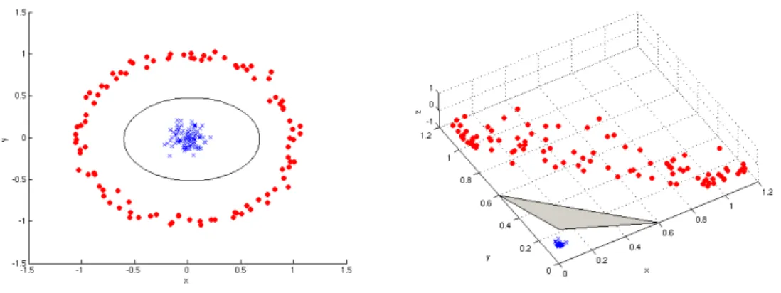
be separated by a linear decision function the already mentioned kernel trick is used to have SVC construct a hyperplane in a feature space, where the mapping to this space is done by
a functionΦ(Figure 2). Since only dot products between patterns are computed in (8) these
dot products can be replaced by kernel function evaluations:
Figure 2: Binary classification problem in input space (left) and the feature space induced by the mappingΦ(x1x2) = (x21,
√
2x1x2, x22)(right). In input space the
two classes can only be separated by a nonlinear decision functionf, an ellipse in this case, whereas in feature space a plane is sufficient for separation of the classes.
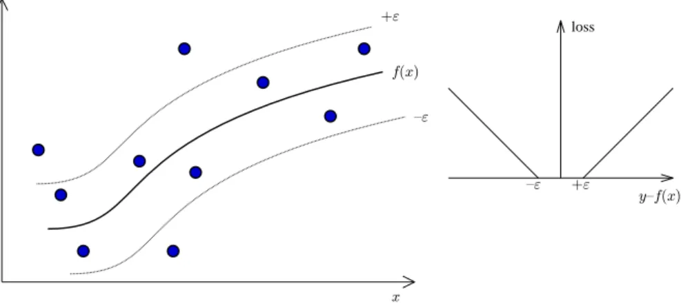
When dealing with regression rather than classification problems the labelsyiare real
val-ues, and the decision functionf is used to predictyion unknown test data. Support Vector
Regression (SVR) therefore computes a function f(x) = hw, xi+b, where the loss is
measured using Vapnik’sε-insensitive loss function (Figure 3):
|y−f(x)|ε= max{0,|y−f(x)| −ε}.
Thus the goal is to find a functionf such that most of the points will lie inside an ε
-tube, which is equivalent to minimizing the loss function. This can be expressed by the
constraintsf(xi)−yi ≤εandyi−f(xi)≤ε. Again it will not be possible to find such
a function for all values ofεmaking it necessary to relax the constraints analogous to the
soft margin classification case. The resulting constrained optimization problem can hence be stated as follows: min w,b,ξ,ξ∗ 1 2kwk 2+C m X i=1 (ξ+ξ∗) subject to f(xi)−yi≤ε+ξi yi−f(xi)≤ε+ξ∗i ξi, ξi∗≥0, ∀i= 1, . . . , m . (9)
Like in SVC the parameterCis used here to trade off between the capacity of the regression
function and the number of violators of theε-tube. Not surprisingly there is an interesting
connection between the margin of SVC and theε-tube of the SVR algorithm [14]. Finally
application of the kernel trick and the introduction of Lagrange multipliers leads to the derivation of the dual optimization problem, which needs to be solved during SVR training:
min α,α∗ 1 2 m X i,j=1 (αi−α∗i)(αj−α∗j)k(xi, xj) +ε m X i=1 (αi+α∗i) + m X i=1 yi(αi−αi∗) subject to m X i=1 (αi−α∗i) = 0 0≤αi, α∗i ≤C, ∀i= 1, . . . , m . (10)
y x " { " + ) x ( f loss ) x ( f { y " { +"
Figure 3:The use of theε-insensitive loss function in SVR corresponds to fitting a
tube of widthεaround the regression functionf(x)to be estimated. Points lying inside of this tube do not contribute to the loss as shown in the inset on the right.
2.1 General formulation forC-SVC andε-SVR
ForC-SVC andε-SVR the dual optimization problem can be stated in the following general
form: min α 1 2α TQα+pTα subject to yTα=δ, 0≤αi≤C, ∀i= 1, . . . , m . (11)
With the kernel matrixQ=yiyjk(xi, xj)forC-SVC it can be clearly seen that the
prob-lem (8) can be restated in the general form above. Following [4] the probprob-lem (10) for
ε-SVR can be reformulated as:
min α,α∗ 1 2 αT(α∗)T Q −Q −Q Q α α∗ + εeT +yT, εeT−yT α α∗ subject to zT α α∗ = 0, 0≤αi, αi∗≤C, ∀i= 1, . . . , m . (12)
wherezis a2mby1vector withyi = 1, i= 1, . . . , mandyi =−1, i=m+ 1, . . . ,2m.
The kernel matrix forε-SVR isQ=k(xi, xj).
2.2 General formulation forν-SVC andν-SVR
Inν-SVC andν-SVR a new parameterνis used to replace the parameterCinC-SVC andε
inε-SVR [14]. The parameterν∈(0,1]allows the direct control of the number of support
vectors and errors. It is an upper bound on the fraction of training errors and a lower bound
of the fraction of support vectors. Forν-SVC the primal problem to be considered is
min w,b,ξ,ρ 1 2kwk 2−νρ+ 1 m m X i=1 ξi subject to yi(hw, xii+b)≥ρ−ξi ξ≥0, ∀i= 1, . . . , m, ρ≥0 (13)
and the corresponding dual
min α 1 2α TQα subject to eTα≥ν, yTα= 0 0≤αi≤1/m, ∀i= 1, . . . , m . (14)
It has been shown [4] that the inequality constraint (14) can be replaced by the equality
eTα=ν. Therefore one can solve the following scaled version of the problem:
min α 1 2α TQα subject to eTα=ν, yTα= 0 0≤αi≤1,∀i= 1, . . . , m . (15)
The solution to the original problem is obtained by rescalingα←α/ρafterwards.
Forν-SVR the primal problem is
min w,b,ξ,ξ∗,ε 1 2kwk 2+C(νε+ 1 m m X i=1 (ξi+ξ∗i)) subject to (hw, xii+b)−yi ≤ε+ξi, (yi− hw, xii+b)≤ε+ξi, ξi, ξi∗≥0, ∀i= 1, . . . , m ε≥0 (16)
and the dual
min α,α∗ 1 2(α−α ∗)TQ(α−α∗) +yT(α−α∗) subject to eT(α−α∗) = 0, eT(α+α∗)≤Cν, 0≤α, α∗≤C/m, ∀i= 1, . . . , m . (17)
Similar to the classification case the inequality can be replaced by an equality. With rescal-ing the actual dual problem to be solved is:
min α,α∗ 1 2(α−α ∗)TQ(α−α∗) +yT(α−α∗) subject to eT(α−α∗) = 0, eT(α+α∗)≤Cmν, 0≤α, α∗≤C, ∀i= 1, . . . , m. (18)
As a result bothν-SVC andν-SVR can be stated in the following general form:
min α 1 2α TQα+pTα subject to yTα=δ1, eTα=δ2, 0≤αi≤C, ∀i= 1, . . . , m . (19)
Before discussing different methods for solving these problems in section 3 it is important
to realize that the general problems to be solved forC-SVC/ε-SVR andν-SVC/ν-SVR just
differ in the number of linear constraints. Theν formulation seems to be harder to solve
since it has two linear constraints. But the structure of the linear constraints is quite simple
and using the fact thatyi∈ {+1,−1}they can be rewritten as:
yTα=δ 1⇔Pyi=+1αi=δ1− P yi=−1αi (20) eTα=δ 2⇔Pyi=+1αi+Pyi=−1αi=δ2. (21)
An initial feasible solution for the problem (19) can thus be easily found by setting
0 ≤ αi ≤ C such thatPyi=+1αi = (δ1+δ2)/2andPyi=−1αi = (δ2−δ1)/2 are
satisfied. If an optimization algorithm now only changes variablesαiwith eitheryi = +1
oryi=−1, but not both at the same time, it is clear that actively maintaining constraint (20)
suffices to ensure that constraint (21) is always satisfied. The reason for this is that
con-straint (20) ensures thatP
vice versaP
yi=−1αi = 0for a change ofαi withyi =−1. Consequently with careful
initialization and change of the optimization variablesαi it is possible to reduce the
opti-mization problem (19) with two linear constraints to the general form given in section 2.1. Unfortunately this reduction thus not work well in practice with some of the QP solvers introduced in section 3 because of numerical problems and the restriction imposed on the variable selection method described above.
3
QP Solvers
There are different approaches to solve the general QP problems given in the last two sub-sections. The interior point algorithm in section 3.1 and gradient projection algorithm in section 3.2 find a numerical solution for the problem, whereas sequential minimal opti-mization (SMO) in section 3.3 finds a solution by sequentially solving two-variable sub-problems, that can be solved analytically themselves.
For all optimization algorithms it is important to decide, when to stop the optimization process. To decide about the optimality of the current solution the so called Karush-Kuhn-Tucker (KKT) conditions are checked [14].
Theorem 1(KKT conditions). : Letf : Rm 7→ Randci : Rm 7→ Rbe functions and L(x, α) = f(x) +Pn
i=1αici(x), αi ≥ 0the corresponding Lagrange function. If there
exists(¯x,α¯), so that:
L(¯x, α)≤L(¯x,α¯)≤L(x,α¯)
thenx¯is a solution to the constrained optimization problem:
minf(x), s.t. ci(x)≤0,∀i= 1, . . . , n .
The relation given in the theorem concerningL(¯x,α¯)just states that the LagrangianLis
minimal w.r.t. ¯xand maximal w.r.t. α¯ at a saddle point. For convex and differentiable
objective functionf and constraintscithe above theorem can be restated.
Theorem 2(KKT conditions for convex differentiable problems). : Letf :Rm7→Rand ci :Rm7→ Rbe convex differentiable functions. Thenx¯is a solution to the optimization
problem
minf(x), subject to ci(x)≤0,∀i= 1, . . . , n ,
if there exists someα¯≥0, such that the following conditions are fulfilled:
∂L(¯x,α¯) ∂x = ∂f(¯x) ∂x + Pn i=1αi ∂ci(¯x) ∂x = 0 (saddlepoint inx¯) (22) ∂L(¯x,α¯) ∂α =ci(¯x) =≤0 (saddlepoint inα¯) (23) Pn i=1α¯ici(¯x) = 0 (KKT gap) (24)
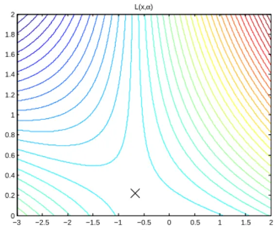
This is the form of the KKT conditions that will be used in the following subsections to derive stopping conditions for the optimization algorithms. But first it might be helpful to look at a simple example in one dimension to understand the implications of the theorem. Example: min x f(x) = 1 2x 2, x∈ R subject to 3x+ 2≤0⇔x≤ −2 3 (25)
A solution to the problem can be found by looking at the constraint, which givesx≤ −2/3.
Sincef(x)is a monotonically decreasing function forx <0the function should reach its
minimum value at pointx = −2/3. To verify that this is an optimal solution the KKT
conditions (22) have to be checked:
L(x, α) = 1/2x2+α(3x+ 2) ∂L(¯x,α¯) ∂x = ¯x+ 3 ¯α= 0 ∂L(¯x,α¯) ∂α = 3¯x+ 2≤0 ¯ α(3¯x+ 2) = 0. (26)
Substitutingx¯ =−2/3results inα¯ = 2/9which satisfy all of the KKT conditions. Thus
¯
xin an optimal solution for the example problem (25). A contour plot ofL(x, α)is given
in figure 4, where the point(−2/3,2/9)obviously is a saddle point ofL(x, α).
x α L(x,α) −3 −2.5 −2 −1.5 −1 −0.5 0 0.5 1 1.5 2 0 0.2 0.4 0.6 0.8 1 1.2 1.4 1.6 1.8 2
Figure 4: Contour plot of the Lagrangian functionL(x, α). A saddle point of
the function is(−2/3,2/9), thusx¯=−2/3is an optimal solution to the example optimization problem given in the text.
3.1 Interior Point Algorithm
The idea of interior point algorithms is based on solving the primal and dual QP problem simultaneously by searching for a pair of primal and dual variables which satisfy both the constraints and the KKT conditions (22). A pair of variables which satisfies primal and dual constraints only is called an interior point. The following exposition of the popular LOQO
interior point algorithm for solving QPs follows [15]. WithA= [yT;eT], b= [δ1;δ2], l=
0,u=Candethe vector of all ones the general problem in equation (19) can be stated as:
min α 1 2α TQα+pTα subject to Aα=b l≤α≤u (27)
By introducing slack variables g, tthe inequalities can be reformulated as equality
con-straints. The resulting primal and dual problem are,
min α,g,t 1 2α TQα+pTα subject to Aα=b α−g=l α+t=u g, t≥0 max y,s,z − 1 2α TQ+bTy+lTz+uTs subject to Qα+p−(Ay)T +s=z s, z≥0 (28)
and the KKT conditions are given by:
gizi= 0, siti= 0, ∀i= 1, . . . , m (29)
The examination of the primal and dual constraints reveals, that an interior point can be found by solving a system of linear equations. Unfortunately the optimal solution cannot
be found directly since the KKT conditions are unsolvable given one of the variables, e.g.
g, s or z, t. As a consequence the KKT conditions are relaxed using a variableµ > 0
which is decreased during the iterative solution process, leading to the two equationsgizi=
µ, siti = µ. Since for a givenµthere is no point in solving (28) exactly one solves the
linearized system which results after expanding variablesαintoα+ ∆αetc.:
A(α+ ∆α) =b α+ ∆α−g−∆g=l α+ ∆α+t+ ∆t=u p+Qα+Q∆α−(A(y+ ∆y))T +s+ ∆s=z+ ∆z (gi+ ∆gi)(zi+ ∆zi) =µ (si+ ∆si)(ti+ ∆ti) =µ (30)
Reformulation of this system yields,
A∆α=b−Aα =:ρ (31) ∆α−∆g=l−α+g =:ν (32) ∆α+ ∆t=u−α−t =:τ (33) (A∆y)T + ∆z−∆s−Q∆α=p−(Ay)T +Qα+s−z =:σ (34) g−1z∆g+ ∆z=µg−1−z−g−1∆g∆z =:γz (35) t−1s∆t+ ∆s=µt−1−s−t−1∆t∆s =:γs (36)
where the notation g−1, t−1 represents component wise inversion, that is g−1 =
(1/g1, . . . ,1/gn), and g−1z, t−1s represents component wise multiplication. Solving
equation (31) for∆g,∆t,∆z,∆sleads to:
∆g=z−1g(γz−∆z) ∆t=s−1t(γs−∆s) ˆ ν=ν+z−1gγz ˆ τ=τ−s−1tγs ∆z=g−1z(ˆν−∆α) ∆s=t−1s(∆α−ˆτ) (37)
Finally∆αand∆yare the solution of the reduced KKT-system [15],
−(Q+g−1z+t−1s) AT A 0 ∆α ∆y = σ−g−1zνˆ−t−1sτˆ ρ (38) which is best solved by Cholesky decomposition [8] and explicit pivoting.
To see how to solve the reduced KKT system let Q1 = Q+g−1z+t−1s, Q2 = 0,
c1=σ−g−1zνˆ−t−1sτˆandc2=ρwhich in conjunction with equation 38 leads to:
−Q1∆α+AT∆y=c1 (39)
A∆α+Q2∆y=c2 (40)
Now solving (39) for ∆α = Q−11(AT∆y−c1) and substituting into (40) ∆y can be
expressed as:
∆y= (AQ−11AT +Q2)−1(c2+AQ−11c1). (41)
Using the Cholesky decompositionQ1 =L1L1T and solution of the systemL1Y1 =AT
the first term in (41) can be computed by:
AQ−11AT+Q2=Y1TLT1L−
T
1 L
−1
With the solutionY2of the triangular systemL1Y2 =c1the second term in (41) can be simplified:
c2+AQ−11c1=c2+ (L1Y1)TL−1TL −1
1 c1=c2+Y1TY2. (43)
As a result∆ycan be determined using the Cholesky decompositionL2LT2 =Y1TY1+Q2
as well as the factorsY1andY2. In the last step when∆yis known∆αcan be computed
by back-substitution:
L2x=c2+Y1TY2
LT2∆y=x
LT1∆α=Y1∆y−Y2.
(44)
During the iterative solution of the QP problem the reduced KKT system is usually solved by a predictor-corrector method. The predictor step involves solving (37) and (38) setting
µ= 0and∆z= ∆s= ∆α= 0on the right hand side, e.g.γz=−zandγs=−s. For
the corrector step the resulting∆-terms are substituted into the definitions ofγzandγsand
the equations (37) and (38) are solved again. At the end of each iteration the∆-terms thus
determined are used to update the valuesα, s, t, z,etc.. The step lengthξfor these updates
is chosen such that the new values do not violate the positivity constraints. A heuristic for
decreasingµis given by [20]: µ= hg, zi+hs, ti 2n ξ−1 ξ+ 10 2 . (45)
Thusµ is decreased rapidly if the average of the feasibility gap given by the first term
is large and if the variables are far away from the boundaries of the positivity constraints
as indicated by a largeξin the second term. Such a decrease hence results in a stronger
enforcement of the KKT conditions.
Starting points for the iterative procedure are found by solving a modified reduced KKT
system (38) by setting auxiliary variables to0:
−(Q+1) AT A 1 α y = p b (46) The positivity of these starting points can be ensured with:
y= max(x, u/100) g= min(α−l, u) t= min(u−α, u) z= min(max(Q+p−(Ay)T,0) +u/100, u) s= min(max(−Q−p+ (Ay)T,0) +u/100, u) (47)
The runtime of the interior point algorithm is dominated by the Cholesky factorization which is the most expensive step during the iterative solution process. As a result LOQO
has a runtime complexity ofO(m3).
3.2 Gradient Projection Algorithm
The gradient projection algorithm uses simple gradient descent for minimizing the
objec-tive functionf(α)w.r.t. the optimization variableα. Feasibility ofαis maintained by
projection on the constraints after each update of the variableα. The two main steps
re-peated by the algorithm are [1]
1. Compute descent directiondt=P
Ω(αt−δt∇f(αt))−αk
wherePΩis the projection operator andδtis the step size found by doing a line-search.
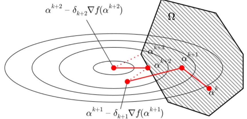
The progress of this algorithm for a simple example is shown in figure 5. Crucial for the practical application of this algorithm are selection of a suitable step size and an efficient
projection operationPon the constraint setΩ.
+3 k ® +2 k ® ) +2 k ® ( f r +2 k ± { +2 k ® ) +1 k ® ( f r +1 k ± { +1 k ® +1 k ® k ®Figure 5:This simple example shows the progress made by the gradient projection
algorithm during the minimization of functionf(α), which is indicated by the contour lines, on the constraint setΩ.
ForC-SVC andε-SVR training the QP problem to be solved has just a single linear
con-straint in equation (11). In [5] they propose suitable step size selection rules and an efficient
projection operation which are used in [23] to solve theC-SVC QP problem by a gradient
projection algorithm.
By exploiting the simple constraint structure of QP problem (19) it is possible to use a
gradient projection algorithm for training ν-SVC and ν-SVR. The idea is to reduce the
projection operation for the two linear constraints to projecting on problems with a
sin-gle linear constraint twice. Given the optimization variableαthe projected variableβ is
obtained by solving the problem
min β 1 2kα−βk 2 subject to yTβ= 0 eTβ=νm 0≤β≤1 (48)
With the substitution ofβi=αi−∆i,∆i ∈Rand usingyi∈ {±1}problem (48) can be
reformulated as: min ∆ 1 2k∆k 2= min ∆ 1 2( X yi=+1 ∆2i + X yi=−1 ∆2i) s.t. X yi=+1 ∆i− X yi=−1 ∆i=yTα=c1 X yi=+1 ∆i+ X yi=−1 ∆i=eTα=c2 αi−1≤∆i≤αi∀i= 1, . . . , m (49)
Now close examination of objective function and constraints reveals that this optimization problem can be split into two smaller optimization problems which are independent of each
other: min 1 2 X yi=+1 ∆2i min 1 2 X yi=−1 ∆2i (50) subject to X yi=+1 ∆2i =1 2(c1+c2) subject to X yi=−1 ∆2i = 1 2(c2−c1) (51) αi−1≤∆i≤αi ∀yi= +1 αi−1≤∆i ≤αi∀yi=−1 (52) With this reduction the QP problem (19) can be solved by the algorithm proposed in [5] the only difference being the number of simple projection operations required.
The gradient projection algorithm exhibits good scaling behavior since the main cost in
each iteration is a matrix-vector product which has a runtime complexity ofO(m2)[23].
Unfortunately the gradient projection algorithm is not suited for solving QP problem (19) in practice due to slow convergence and numerical problems.
3.3 Sequential Minimal Optimization
The SMO algorithm proposed by [13] solves QP problem (11) by sequential optimization of only two variables while the values of all other variables are fixed. A solution for the QP problem in two variables can be found analytically and the choice of variables selected in each iteration is guided by the violation of the KKT conditions (22). The optimization problem (11) in two variables can be stated as follows:
min 1 2(αiαj) Qii Qij Qij Qjj αi αj + (pB+QBNαN) αi αj (53) subject to yiαi+yjαj=δ−yTNαN (54) 0≤αi, αj ≤C . (55)
IfI ={1, . . . , m} denotes the index set of all variables thenB ={i, j} is the index set
of those variables currently optimized andN =I\B is the index set of fixed variables.
To analytically solve this problem the first step consists of expressing the objective
func-tion (53) in dependence of only one optimizafunc-tion variableαi. Thus the starting point is the
objective function which can be rewritten as
f(αi, αj) =
1 2(α
2
iQii+ 2αiαjQij+α2jQjj) +ciαi+cjαj , (56)
where the constantsci, cjare given by:
ci= ((pB+QBN)αN)i=∇f(α)i−Qiiαoldi −Qijαoldj
cj = ((pB+QBN)αN)j =∇f(α)j−Qijαoldi −Qjjαoldj ,
(57)
and αold is the value of the optimization variables at the previous optimization step.
Because of constraint (54) variable αj can be expressed byαj = yj(γ −yiαi), γ =
(yjαoldi +yjαoldj )andαjcan be eliminated in (56) yielding:
f(αi) = 1 2α 2 iQii+αi(yjγ−yiyjαi)Qij+ 1 2(yjγyiyjαi) 2Q jj+ciαi+cj(yjγ−yjyiαi) = 1 2α 2 i(Qii−2yiyjQij+Qjj) +αi(yjγQij−yiγQjj+ci−cjyiyj) +1 2γ 2Q jj+cjyjγ .
Now the location of the minimum forf(αi)is determined by computing the derivative,
setting it to zero and solving forαi:
f0(αi) =αi(Qii−2yiyjQij+Qjj) + (yjγQij−yiγQjj+ci−cjyiyj) ! = 0 (58) ⇒αi= yiγQjj−yjγQij−ci+cjyiyj Qii−2yiyjQij+Qjj (59)
A similar expression can be derived forαj via elimination ofαiin the objective function.
To get update equations for αi andαj it is beneficial to distinguish between two cases,
namelyyi=yjandyi6=yj: yi =yj: αi= yiγQjj−yjγQij−ci+cj Qii−2Qij+Qjj = α old i (Qii−2Qij+Qjj) +∇f(α)j− ∇f(α)i Qii−2Qij+Qjj =αoldi +∇f(α)j− ∇f(α)i Qii−2Qij+Qjj αj=αoldj + ∇f(α)i− ∇f(α)j Qii−2Qij+Qjj yi 6=yj: αi= yiγQjj−yjγQij−ci−cj Qii+ 2Qij+Qjj = α old i (Qii+ 2Qij+Qjj)− ∇f(α)i− ∇f(α)j Qii+ 2Qij+Qjj =αoldi + −∇f(α)i− ∇f(α)j Qii+ 2Qij+Qjj αj=αoldj + −∇f(α)i− ∇f(α)j Qii+ 2Qij+Qjj
In the next step after updating the optimization variables one has to ensure that
con-straints (54) and (55) are satisfied. Withαj=yj(γ−αiyi)and0≤αj≤Cthe following
constraints forαiare derived:
yiyjαoldi +α old j −C≤yiyjαi≤yiyjαoldi +α old j (60) 0≤αi≤C . (61)
Again the discussion is simplified by considering casesyi =yj andyi 6=yj separately.
Foryi=yjthe constraints (60) can be combined into:
max(0, σ−C)≤αi≤min(C, σ), withσ=αoldi +αoldj . (62)
Since by construction of the optimal solutionαj =αoldi +α
old
j −αi=σ−αiforyi =yj
the decision on how to changeαi, αj to satisfy the constraints can be solely based on the
value ofσandαi. The result of this reasoning are the following update rules forαiandαj:
σ > C: αi<0 :αi←σ−C, αj ←C αi> C :αi←C, αj←σ−C σ < C: αi<0 :αi←0, αj ←σ αi> C :αi←σ, αj ←0.
Foryi6=yjsimilar update rules can be derived from on the combined constraint
leading to: ρ >0 : αi<0 :αi←ρ, αj←0 αi> C :αi←C, αj ←C−ρ ρ <0 : αi<0 :αi←0, αj←ρ αi> C :αi←C+ρ, αj ←C .
With these update rules the only missing pieces to complete SMO are a suitable stopping
condition for the optimization loop and a selection criterion forαi, αj. The stopping
con-dition is derived for (53) from the general KKT concon-ditions in theorem 2. The Lagrangian in this case is:
L(α, b, λ, µ) =1 2α
TQα+pTα−b(δ−yTα)−λα−µ(C−α). (64)
Application of theorem 2 results in the following KKT conditions:
∂L ∂α =∇f(α) +by−λ+µ= 0⇔ ∇f(α) +by=λ−µ (65) ∂L ∂b =y Tα−δ= 0 (66) ∂L ∂λ =−α≤0⇔α≥0 (67) ∂L ∂µ =α−C≤0⇔α≤C (68) m X i=1 µi(C−αi) + m X i=1 λiαi+ m X i=1 yiαi−δ= 0 (69)
Combining conditions (66) and (69) leads toµi(C−αi) = 0, µi≥0andλiαi= 0, λi≥0
for alli. Closer analysis of these conditions reveals the following identities:
λiαi= 0⇔(αi= 0∧λi>0)∨(αi>0∧λi= 0)
µi(C−αi) = 0⇔(αi=C∧µi>0)∨(αi< C∧µi= 0)
⇒λi−µi≥0⇔αi < C
⇒λi−µi≤0⇔αi >0
Since∇f(αi) +byi ≥ 0 ⇔ λi−µi ≥ 0and∇f(αi) +byi ≤ 0 ⇔ λi −µi ≤ 0by
condition (65) with the aid of the identities above this KKT condition can be reformulated as
∇f(α)i+b≥0∀i∈Iup={i|(αi< C∧yi = +1)∨(αi>0∧yi=−1} (70)
∇f(α)i+b≤0∀i∈Ilow={i|(αi>0∧yi= +1)∨(αi< C∧yi=−1} (71)
exploiting the fact thatyi∈ {±1}. With these definitions a suitable stopping condition for
the optimization procedure is given by:
max
i∈Iup
(−yi∇f(α)i)− min i∈Ilow
(−yi∇f(α)i)≤ (72)
where is a small positive constant which controls to what extent the KKT conditions
have to be fulfilled before stopping the optimization procedure. The variablesαi, αjto be
optimized in each step are those that maximize the progress w.r.t. the KKT gap. Therefore these variables are often called the ’maximal violating pair’ given by:
i= arg max i∈Iup (−yi∇f(α)i) j= arg min j∈Ilow (−yj∇f(α)j)
In comparison to the interior point algorithm in section 3.1 and the gradient projection al-gorithm in section 3.2 SMO has the big advantage of not running into numerical problems due to its analytical nature. Empirical experiments [13] with datasets of different sizes have
shown, that SMO scales roughly withO(m2)in practice. Unfortunately its sequential
so-lution procedure does not lead to straightforward parallelization strategy for this algorithm. Despite this disadvantage the algorithm can be nonetheless successfully employed as inner solver for a decomposition based parallelization strategy.
4
Decomposition for large scale SVM training
In principle all the methods described in section 3 can be used to train SVMs for classifi-cation and regression tasks. Yet the interior point algorithm in section 3.1 and the gradient
projection algorithm in section 3.2 are not suited to solve large scale problems with105
-106patterns in practice due to their runtime complexities ofO(m3)andO(m2). Another
issue is the storage requirement of the kernel matrix. A dataset with60000patterns requires
more than13GB of memory for example if each entry is assumed to be a single precision
floating point value.
To deal with these issues [11] introduced a decomposition method for breaking down the original QP problem into several smaller problems
min 1 2α T B QBB QBN QN B QN N αB+ (pB+QBNαN)αB (73) subject to yTBαB =δ−yNTαN (74) 0≤αB ≤C . (75)
whereB is the index set of the currently optimized variables andN the index set of the
fixed variables. The SMO algorithm explained in section 3.3 essentially uses this decom-position idea in the extreme case where each subproblem has size two. To avoid storing the complete kernel matrix in main memory [11] proposes a caching scheme where only the most recently used kernel matrix rows are stored in memory.
Solving each of the subproblems arising in the decomposition approach can be done with all of the algorithms described in section 3. The only remaining question to be answered
concerns the selection of an appropriate working setB and a stopping condition for the
decomposition approach.
4.1 Working set selection
For the selection of the working setBthe reasoning given in section 3.3 for the ’maximal
violating pair’ can be generalized for selecting more than two variables. Sorting the index
setI of all optimization variables into a list in decreasing order w.r.t. −yi∇f(α)i and
selecting pairs of variables, where the first variable is from the top of the list withi∈Iup
and the second variable is from the bottom of the list withi∈Ilow, results in a working set
Bwhere each pair is in some sense a ’maximal violating pair’. With this selection strategy
it is possible to fill the working set with more than two variables, but the number of selected variables might be less than the required working set size. Consequently, if necessary, the
working set is filled up with the most recent indices1in the previous working set that are
not yet inB, where preference is usually given to free variables [23].
Another important point of the working set selection strategy is the number of new variables
nthat enter the working set at each step. Ifnis chosen to be equal to the size of the working
set (n=|B|=q) a so called ’zigzagging’ of variables might occur, that is, some variables
might enter and leave the working set for many times which in turn can slow down the
optimization algorithm considerably. A suitable initial value fornthat works in practice
isn= q/2. To get faster convergencenis decreased during the optimization process as
1
described in [23]. With these considerations in mind the strategy for selectingB can be summarized as follows:
1. Letqbe the required working set size andnthe number of new variables to enter
the working set.
2. Sort the index setIinto decreasing order w.r.t.−yi∇f(α)iand let(i1, . . . , in)be
the sorted index sequence.
3. Select pairs(iu, il)of indices withl < ufrom the sequence whereiu ∈Iupand
il ∈ Ilow untilnindices are selected or no pair satisfying the above conditions
can be found.
4. LetB0be the working set selected so far.
5. If|B0| < qfill upB0with the most recent indicesi∈B\B0with0< αi < C
(free variables).
6. If|B0| < n fill upB0 with the most recent indicesi ∈ B \B0 withα
i = 0
(variables at lower bound).
7. If|B0| < nfill upB0 with the most recent indices i ∈ B \B0 withαi = C
(variables at upper bound).
8. Adapt n by settingn = min(n,max(10, q0, n0)), whereq0 is the largest even
integer withq0 < q/10 andn0 is the largest even integer with n0 < |{i, i ∈
B0\B}|. SetB=B0.
4.2 Stopping condition
As stopping condition for the decomposition approach the stopping condition (72) for the
SMO algorithm in section 3.3 can be used. In this case the index setsIup andIlow are
subsets of the whole index setI=B∪N.
5
Implementation
It was already pointed out in the last section that the decomposed QP problem (73) can be solved by all of the QP solvers described in section 3. After implementing these algo-rithms it becomes apparent that not all are suited to solve large scale SVM problems in practice. This section gives some hints on why the interior point algorithm and the gradient projection algorithm are not the first choice in practice and explain why a parallel SMO implementation should be preferred.
In [23] the gradient projection algorithm exhibits a very good parallel behavior for large
scaleC-SVC training. With the reformulation forν-SVC given in section 3.2 it is possible
to apply the gradient projection algorithm to the problem of large scaleν-SVC training. For
the sequential implementation of this approach the code2of [23] is modified accordingly.
Unfortunately the two step projection for solving theν-SVC problem does not work well
in practice. At least it only works for some datasets and settings of the parameterν while
on most datasets this approach failed to converge due to numerical problems. Therefore the gradient projection algorithm is not considered any further in this study.
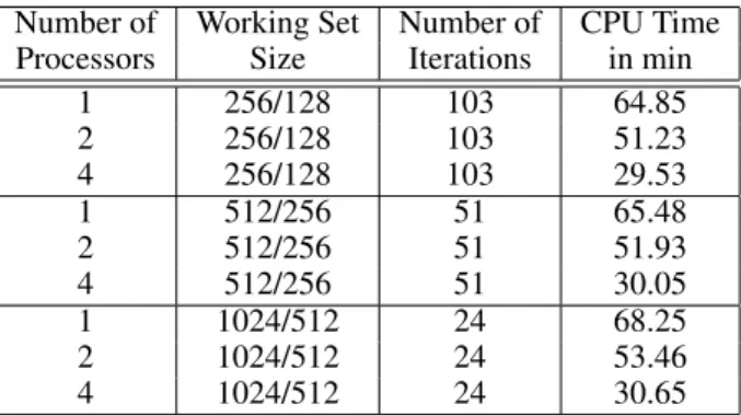
The LOQO interior point algorithm described in section 3.1 is implemented using the par-allel linear algebra library PLAPACK [19]. This library contains a very good parpar-allel Cholesky solver for dense matrices which is essential for solving the reduced KKT system. Testing this approach on several large scale datasets with different sizes of the working set
reveals that there is a linear relationship3between the working set size and the number of
iterations required by the decomposition approach to converge (Table 1). Therefore one could expect a linear speedup when increasing the working set size which is not observed in practice as the runtime on a fixed number of processors is almost constant. This is caused
by the runtime complexity of the interior point algorithm which scales withO(m3), where
2
Available at:http://dm.unife.it/gpdt/ 3
Number of Working Set Number of CPU Time
Processors Size Iterations in min
1 256/128 103 64.85 2 256/128 103 51.23 4 256/128 103 29.53 1 512/256 51 65.48 2 512/256 51 51.93 4 512/256 51 30.05 1 1024/512 24 68.25 2 1024/512 24 53.46 4 1024/512 24 30.65
Table 1:Performance of the decomposition approach using LOQO as inner solver
for the dataset mnist-576-rbf-8vr.
in this casemis the number of variables in the working set. When increasing the number
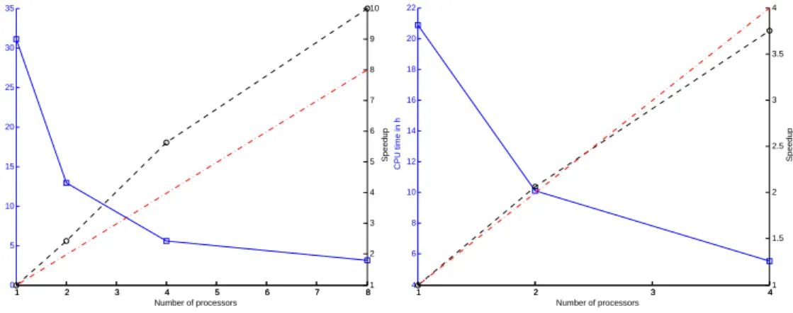
of processors the runtime complexity of LOQO also explains the bad parallel performance. Figure 6 shows the results of LOQO in comparison to parallel SMO (described next) on one of the MNIST datasets (cf. section A). In addition to this LOQO has convergence
problems on a subset of theν-SVC tasks and for certain values of the parameterν.
Figure 6: Comparison of LOQO and parallel SMO (PSMO) with respect to
run-time (left) and speedup (right) on the mnist-576-rbf-8vr dataset. Due to theO(m3)
runtime complexity of LOQO the parallel decomposition approach using LOQO as inner solver does not scale well. On the other hand PSMO is able to achieve a superlinear speedup for this dataset. The size of the working set in both cases is
q= 512and the number of new variables entering the working set isn= 256.
To avoid the problems just mentioned a parallel implementation of the SMO algorithm de-scribed in section 3.3 can be used. This approach will be termed PSMO in the following discussion. It is based on the observation that in practice the main computational bur-den is not the solution of the inner QP problem, as long as the working set size is small
and contains about256−2048variables. Profiling information gathered for the parallel
implementations on different datasets indicates that the computational bottleneck are the
kernel evaluations which are needed to update the gradient∇f(α). Note that updating
the gradient is essential for the working set selection and the evaluation of the stopping
condition (72). The profiling information reveals that between90−98% of the runtime is
spend on updating the gradient. This is the motivation for PSMO which uses the sequential SMO algorithm for solving the subproblems arising in the decomposition approach while performing problem setup, kernel evaluations, caching of kernel rows and gradient updates in parallel. Important for achieving good speedups is a good load balancing between the processors which in PSMO achieves by a distributed caching strategy.
The distributed caching strategy basically assigns the computational tasks with a round-robin strategy. Before the gradient is updated in each iteration the following steps are executed:
1. Each processor determines the kernel rows with indices in the current working set
B, which are cached/not cached locally.
2. Next the local cache information is synchronized across all processors.
3. Using the global cache information the index setB is split into cachedBc and
non-cachedBncindices.
4. Bcis distributed among the processors with a round-robin strategy4Let the
result-ing sets beBlocal
c andBnclocal.
5. Then each processor updates all components of∇f(α)i, with indexi∈Blocalc ∪
Blocal
nc . Cached entries are updated before the non-cached ones.
6. Finally the gradient∇f(α)is synchronized between all processors.
PSMO was implemented using a modified SMO from the LibSVM [4] software version 2.8. One change of the LibSVM library involves the the sparse data representation, which is
replaced by a new sparse data structure recommended by the BLAS Technical Forum.5 All
communication that is necessary between the processors for the distributed caching strategy and data synchronization is implemented using the Message Passing Interface (MPI) [7].
6
Results
The results presented in the following subsections forC-SVC,ν-SVC ,ε-SVR andν-SVR
are all based on the PSMO implementation of section 5. For classification four datasets mnist-576-rbf-8vr, mnist-784-poly-8vr, covtype-2vr and kddcup99-nvr are used. The two regression datasets are kddcup98 and mv (for details cf. section A). All performance tests
are run on the Kepler6cluster, which has 32 Dual AMD Athlon MP 2000+ nodes with 1666
MHz , 256 L2 Cache and 1-2GB RAM running Linux (2.4.21 kernel). Communication between nodes occurs over a Myrinet interconnect with MPI Peak performance of 115MB per second and node. Because of technical reasons it is not possible to run programs on
more than8processors. Therefore in the following all performance results are given for up
to8processors. The size of the distributed cache is set to256MB for all tests.
4First processor gets first index, second processor gets second index etc., wrapping around if
necessary.
5
http://www.netlib.org/blas/blast-forum/
6
6.1 C-SVC
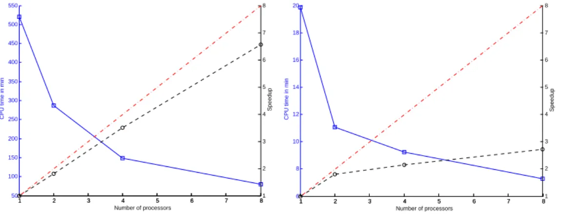
Parallel solution of theC-SVC problem for the classification datasets mnist-576-rbf-8vr,
mnist-784-poly-8vr and covtype-2vr with PSMO yields a superlinear speedup on up to8
processors as shown in figure 7 and figure 8. For the kddcup99-nvr an almost linear speedup
is achieved on up to4processors (figure 8). The parameters used for training PSMO and
LibSVM on the four datasets are given in table 2. To put these speedups in relation to LibSVM performance on a single processor, the runtime of LibSVM on one CPU is also measured and listed in table 3. On both MNIST datasets the single processor runtime of PSMO is better than that of LibSVM, whereas on the other two datasets LibSVM outper-forms PSMO in the sequential case. But it is important to note that the single processor runtime of PSMO on these datasets could be potentially improved by choosing a different working set size. Nonetheless PSMO on four processors is still twice as fast as LibSVM on a single processor for the covtype-2vr dataset and a constant two hours faster for the kddcup99-nvr dataset.
Dataset C-SVC Parameters Working Set Size
mnist-576-rbf-8vr C= 10,γ= 1.667 512/256
mnist-784-rbf-8vr C= 10,d= 7 512/256
covtype-2vr C= 10,γ= 2e−5 1024/512
kddcup99-nvr C= 2,γ= 0.6 512/256
Table 2: PSMO and LibSVM training parameters and working set size for the
C-SVC problems
Dataset CPU Time Test Error
PSMO LibSVM v2.8 PSMO LibSVM v2.8
mnist-576-rbf-8vr 59.13 [m] 103.5 [m] 99.82% 99.82%
mnist-784-rbf-8vr 126.24 [m] 153.90 [m] 99.51% 99.51%
covtype-2vr 31.12 [h] 11.71 [h] 96.35% 96.36%
kddcup99-nvr 20.89 [h] 7.369 [h] 92.71% 92.71%
Table 3:Single processor CPU Time and test error for PSMO in comparison with
LibSVM v2.8 for theC-SVC problems.
1 2 3 4 5 6 7 8 0 10 20 30 40 50 60 Number of processors
CPU time in min
1 2 3 4 5 6 7 80 2 4 6 8 10 12 14 16 Speedup 1 2 3 4 5 6 7 8 0 20 40 60 80 100 120 140 Number of processors
CPU time in min
1 2 3 4 5 6 7 80 5 10 15 20 25 Speedup
Figure 7:C-SVC Speedup and CPU time for dataset mnist-576-rbf-8vr (left) and
1 2 3 4 5 6 7 8 0 5 10 15 20 25 30 35 Number of processors CPU time in h 1 2 3 4 5 6 7 81 2 3 4 5 6 7 8 9 10 Speedup 1 2 3 4 4 6 8 10 12 14 16 18 20 22 Number of processors CPU time in h 1 2 3 41 1.5 2 2.5 3 3.5 4 Speedup
Figure 8: C-SVC Speedup and CPU time for dataset covtype-tr-2vr (left) and
dataset kddcup99-nvr (right).
6.2 ν-SVC
Table 4 summarizes the parameters used for ν-SVC training on the four classification
datasets. As shown in figure 9 and figure 10 superlinear speedups are achieved again on up to 8 processors. The only exception being the runtime for the mnist-576-rbf-8vr dataset where a superlinear speedup is observable for up to 4 processors. Comparison of single
processor runtime with LibSVM shows the same situation as for C-SVC where PSMO
runtime for mnist-576-rbf-8vr and mnist-784-poly-8vr is better than LibSVM.
Dataset ν-SVC Parameters Working Set Size
mnist-576-rbf-8vr ν = 0.002356,γ= 1.667 512/256
mnist-784-rbf-8vr ν = 0.006753,d= 7 512/256
covtype-2vr ν = 0.131544,γ= 2e−5 1024/512
kddcup99-nvr ν= 0.001164,γ= 0.6 512/256
Table 4: PSMO and LibSVM training parameters and working set size for the
ν-SVC problems
Dataset CPU Time Test Error
PSMO LibSVM v2.8 PSMO LibSVM v2.8
mnist-576-rbf-8vr 40.76 [m] 98.55 [m] 99.82% 99.82%
mnist-784-rbf-8vr 87.05 [m] 153.60 [m] 99.51% 99.51%
covtype-2vr 25.06 [h] 23.72 [h] 96.34% 96.33%
kddcup99-nvr 43.89 [h] 23.35[h] 92.71% 92.71%
Table 5:Single processor CPU Time and test error for PSMO in comparison with
LibSVM v2.8 for theν-SVC problems.
The difference in runtime for covtype-2vr is about two hours whereas LibSVM is twice as fast on kddcup99-nvr. When PSMO is run in parallel on 4 processors the runtime for kddcup99-nvr is cut down to 10 hours, which is twice as fast as the runtime of LibSVM. The test error reported in table 2 indicates that the parallelization technique employed in PSMO does not influence the classification performance.
1 2 3 4 5 6 7 8 5 10 15 20 25 30 35 40 45 Number of processors
CPU time in min
1 2 3 4 5 6 7 81 2 3 4 5 6 7 8 Speedup 1 2 3 4 5 6 7 8 0 10 20 30 40 50 60 70 80 90 Number of processors
CPU time in min
1 2 3 4 5 6 7 80 2 4 6 8 10 12 14 Speedup
Figure 9:ν-SVC Speedup and CPU time for dataset mnist-576-rbf-8vr (left) and
dataset mnist-784-poly-8vr (right).
1 2 3 4 5 6 7 8 0 5 10 15 20 25 30 Number of processors CPU time in h 1 2 3 4 5 6 7 81 2 3 4 5 6 7 8 9 10 Speedup 1 2 3 4 10 15 20 25 30 35 40 45 Number of processors CPU time in h 1 2 3 41 1.5 2 2.5 3 3.5 4 4.5 Speedup
Figure 10: ν-SVC Speedup and CPU time for dataset covtype-2vr (left) and
dataset kddcup-nvr (right).
6.3 ε-SVR
Training parameters used forε-SVR on the datasets kddcup98 and mv are listed in table 6.
The performance comparison of PSMO with LibSVM on a single processor shows that there is no difference in training time for the mv dataset. For the kddcup98 dataset PSMO is approximately three times as fast as LibSVM while the quality difference of the results, in terms of mean squared error (MSE) on the test set, is negligible (table 7).
Dataset ε-SVR Parameters Working Set Size
kddcup98 C= 0.0078,ε= 0.01,γ= 13.6436 512/256
mv C= 32,ε= 0.01,γ= 0.1084 512/256
Table 6: PSMO and LibSVM training parameters and working set size for the
ε-SVR problems
It can be seen in figure 11 that the speedup of PSMO for theε-SVR is not linear for both
datasets. For the mv dataset this can be attributed to the low speedup potential of this dataset that manifests itself in the small number of input patterns and low dimensionality of the data on the one hand and the short single processor runtime of about 20 minutes on the other hand. But this argumentation cannot be used to explain the behavior of PSMO on the kddcup98 dataset. Here one could speculate that the distributed caching strategy does not
Dataset CPU Time Test MSE
PSMO LibSVM v2.8 PSMO LibSVM v2.8
kddcup98 8.671 [h] 29.51[h] 6.06e-04 6.07e-04
mv 19.86 [m] 20.0 [m] 3.15e-05 3.24e-05
Table 7:Single processor CPU Time and test error for PSMO in comparison with
LibSVM v2.8 for theε-SVR problems.
work well, when the fraction of support vectors is low. Since for kddcup98 approximately half of the input patterns end up as support vector this cannot explain the lower speedup achieved by PSMO on this datasets and further investigations are necessary to elucidate the relationship between speedup and dataset properties.
1 2 3 4 5 6 7 8 50 100 150 200 250 300 350 400 450 500 550 Number of processors
CPU time in min
1 2 3 4 5 6 7 81 2 3 4 5 6 7 8 Speedup 1 2 3 4 5 6 7 8 6 8 10 12 14 16 18 20 Number of processors
CPU time in min
1 2 3 4 5 6 7 81 2 3 4 5 6 7 8 Speedup
Figure 11:ε-SVR Speedup and CPU time for dataset kddcup98 (left) and dataset
mv (right).
6.4 ν-SVR
The training ofν-SVR on the datasets mv and kddcup98 yields results with quality similar
toC-SVR when the parameters given in table 8 are used. When viewed with respect to
runtime and speedup the results give the same picture as forC-SVR the only exception
being the runtime of LibSVM for the mv dataset which is about four times as high as in the
C-SVR case. The statements made about the speedup potential of the datasets in section 6.3
also hold for the parallelν-SVR training.
Dataset ν-SVR Parameters Working Set Size
kddcup98 C= 0.0078,ν= 0.092862,γ= 13.6436 512/256
mv C= 32,ν = 0.020947,γ= 0.1084 512/256
Table 8: PSMO and LibSVM training parameters and working set size for the
Dataset CPU Time Test MSE
PSMO LibSVM v2.8 PSMO LibSVM v2.8
kddcup98 8.983 [h] 29.85[h] 6.05e-04 6.06e-04
mv 24.43 [m] 82.60 [m] 3.24e-05 3.21e-05
Table 9:Single processor CPU Time and test error for PSMO in comparison with
LibSVM v2.8 for theν-SVR problems.
1 2 3 4 5 6 7 8 50 100 150 200 250 300 350 400 450 500 550 Number of processors
CPU time in min
1 2 3 4 5 6 7 8 1 2 3 4 5 6 7 8 Speedup 1 2 3 4 5 6 7 8 10 15 20 25 Number of processors
CPU time in min
1 2 3 4 5 6 7 8 1 2 3 4 5 6 7 8 Speedup
Figure 12:ν-SVR Speedup and CPU time for dataset kddcup98 (right) and dataset
mv (left).
7
Conclusion
This article described various ways how to parallelize SVM training for the original
non-simplified SVM formulations includingC-SVCν-SVC,ε-SVR andν-SVR. Three
differ-ent parallelization strategies arise from the use of the interior point algorithm, the gradidiffer-ent projection algorithm or SMO in combination with the decomposition approach for SVM training. While the gradient projection algorithm has already been successfully used for
parallelC-SVC section 3.2 described how to extend the algorithm to solve QP problems
with two linear constraints that need to be solved when trainingν-SVC andν-SVR.
Al-though this extension is theoretically possible it does not work in practice due to slow convergence. Similar practical experience with the parallel LOQO implementation of the interior point algorithm and the careful analysis of profiling information have led to the im-plementation of PSMO. Despite the fact that PSMO uses a sequential inner QP solver it is
possible to achieve superlinear speedups forC-SVC andν-SVR. In the regression setting
PSMO showed close to linear speedup on the examined kddcup98 dataset while on the mv dataset it is still unclear why only moderate speedups are obtained. Further work is needed to elucidate the relationship between speedup and properties of the dataset. Another impor-tant point to investigate in the future concerns an optimal parallelization strategy in terms of speedup or runtime for multi-class problems.
A
Description of datasets
An overview of all the datasets used in this study is given in table 10. Datasets were selected to ease comparison with similar studies like [23, 17]. The preprocessing of each dataset and the selection of SVM parameters are described in detail in the following subsections. All
datasets are available for download athttp://pisvm.sourceforge.net. Pointers
to the original sources of the datasets are provided at the same location. Kernels used for
these datasets include the RBF kernelk(xi, xj) =e−γkxi−xjk
2
and the polynomial kernel
k(xi, xj) =hxi, xji d
Dataset Number of Patterns Number of Dimensions Train Test mnist-576-rbf-8vr 60000 10000 576 mnist-784-poly-8vr 60000 10000 784 covtype-2vr 435759 145253 54 kddcup99-nvr 4898430 311029 122 kddcup98 95412 96367 403 mv 36768 4000 10
Table 10:Overview of dataset size and dimension.
A.1 mnist-576-rbf-8vr and mnist-784-poly-8vr
Both datasets originate from the MNIST dataset for handwritten digit recognition and only differ in the type of preprocessing that is done. For mnist-576-rbf-8vr which is used in
con-junction with the RBF kernel a576-dimensional discriminative feature vector is extracted
from the original data [6]. The dataset mnist-784-poly-8vr is prepared by centering each
digit image in a28×28box, smoothing with a3×3mask (center element 1/2, rest 1/16)
and normalizing each pattern, such that its dot product is always within[0,1][6]. SVC
parameters areC = 10for both datasets,γ = 1.667for mnist-576-rbf-8vr andd= 7for
mnist-784-poly-8vr and are determined using cross-validation on a subset of the training
data [6]. Finally the10-class problem of the MNIST dataset is reduced to a2-class problem
by separating digit8from the rest [23].
A.2 covtype-2vr
The task of distinguishing between8 different classes of forest covertype is represented
by the covtype dataset. For the conversion to a binary problem class2is to be separated
from the other classes. Preparation of the dataset and choice of SVM parameters is done as
described in [23]. The RBF kernel is used with parameterγ = 2e−5, the regularization
parameter of the SVC is set toC= 10and the stopping condition is= 0.01.
A.3 kddcup99-nvr
The kddcup99-nvr dataset is based on an intrusion detection problem. During
preprocess-ing of the dataset it became apparent that pattern4817100 obviously contained data
for-matting errors and was removed from the training dataset. Furthermore symbolic features in the original dataset are converted to unary coded features and all features are scaled to
lie in the interval[0,1]following [18]. Parameters are set as in [23] withγ= 0.6,C= 2
and stopping condition= 0.01.
A.4 kddcup98
This regression dataset was originally provided by the Paralyzed Veterans of America (PVA) a non-profit organization that provides programs and services for US veterans with spinal cord injuries or diseases. Since most of the funding of PVA is raised by mailing donors the goal is to maximize the donated money in dependence of behavioral and social features of the donors. By including only numerical features the original dataset is
re-duced to contain403features. Missing values are imputed by replacing them by the mean
of the given values. Then the features and target values are scaled to lie in the interval
[0,1]. To estimate the RBF kernel parameterγthe method proposed in [18] is used, that
isγ = 1/(1/m2)Pm
i,j=1kxi −xjk2, leading toγ = 13.6436for this dataset. Finally
SVR parameters are selected by5-fold cross-validation withC ∈ {2−7,2−5, . . . ,27}and
ε ∈ {0.01} resulting inC = 2−7andε = 0.01. All parameters are selected on a1000
A.5 mv
Estimation of SVR parameters follows the description given in section A.4 for dataset
kddcup98 and results inγ = 0.1084,C = 32andε = 0.01. The dataset is an artificial
regression task with dependencies among the features.
References
[1] Dimitri P. Bertsekas. Nonlinear Programming. Athena Scientific, second edition,
2003.
[2] A. Bode. Multicore-Architekturen. Informatik Spektrum, 29(5):349–352, October
2006.
[3] Mihai B˘adoiu and Kenneth L. Clarkson. Smaller core-sets for balls. In SODA
’03: Proceedings of the Fourteenth Annual ACM-SIAM Symposium on Discrete Algo-rithms, 2003.
[4] Chih-Chung Chang and Chih-Jen Lin. LIBSVM: a Library for Support Vector Ma-chines, 2006. Software available at
http://www.csie.ntu.edu.tw/˜cjlin/libsvm.
[5] Yu-Hong Dai and Roger Fletcher. New algorithms for singly linearly constrained
quadratic programs subject to lower and upper bounds. Math. Progm. Ser. A,
(106):403–421, October 2005.
[6] Jian-Xiong Dong, Adam Krzyzak, and Ching Y. Suen. Fast SVM Training Algorithm
with Decomposition on Very Large Data Sets.IEEE Transactions on Pattern Analysis
and Machine Intelligence, 27(4):603–618, April 2005.
[7] Message Passing Interface Forum. MPI: A message-passing interface standard. Tech-nical Report UT-CS-94-230, 1994.
[8] Gene H. Golub and Charles F. van Loan. Matrix Computations. The John Hopkins
University Press, third edition, 1996.
[9] Hans Peter Graf, Eric Cosatto, Leon Bottou, Igor Durdanovic, and Vladimir Vapnik.
Parallel Support Vector Machines: The Cascade SVM. Advances in Neural
Informa-tion Processing Systems, 17, 2005.
[10] Thomas G¨artner, Peter Flach, and Stefan Wrobel. On Graph Kernels: Hardness
Re-sults and Efficient Alternatives. In B. Sch¨olkopf and M.K. Warmuth, editors,
Pro-ceedings of the 16th Annual Conference on Computational Learning Theory and 7th Kernel Workshop, pages 129–143, Stanford University, CA, USA, 2003. Springer Verlag.
[11] T. Joachims. Making large-scale support vector machine learning practical. In
A. Smola B. Sch¨olkopf, C. Burges, editor, Advances in Kernel Methods: Support
Vector Machines. MIT Press, Cambridge, MA, 1998.
[12] O. L. Mangasarian and David R. Musicant. Active support vector machine
classifica-tion. InNIPS, pages 577–583, 2000.
[13] J. Platt. Fast training of SVMs using sequential minimal optimization. In A. Smola
B. Sch¨olkopf, C. Burges, editor,Advances in Kernel Methods: Support Vector
Ma-chines. MIT Press, Cambridge, MA, 1999.
[14] Bernhard Sch¨olkopf and Alexander J. Smola.Learning with Kernels – Support Vector
Machines, Regularization, Optimization, and Beyond. MIT Press, first edition edition, 2002.
[15] A. J. Smola.Learning with Kernels. PhD thesis, Technische Universit¨at Berlin, 1998.
[16] John Shawe Taylor and Nello Cristiaini. Kernel Methods for Pattern Analysis.
Cam-bridge University Press, 2004.
[17] Ivor W. Tsang, James T. Kwok, and Pak-Ming Cheung. Core Vector Machines: Fast
SVM Training on Very Large Data Sets. Journal of Machine Learning Research,
[18] Ivor W. Tsang, James T. Kwok, and Kimo T. Lai. Core Vector Regression for Very
Large Regression Problems. InProceedings of the22ndInternational Conference on
Machine Learning, pages 913–920, 2005.
[19] Robert A. van de Geijn. Using PLAPACK: Parallel Linear Algebra Package. The
MIT Press, 1997.
[20] R. J. Vanderbei and D. F. Shanno. An interior-point algorithm for nonconvex nonlin-ear programming. Technical Report SOR-97-21, Princeton University, 1997.
[21] Vladimir N. Vapnik. The Nature of Statistical Learning Theory. Springer, second
edition, 1999.
[22] G. Zanghirati and L. Zanni. A parallel solver for large quadratic programs in training
support vector machines.Parallel Computing, (29):535–551, 2002.
[23] Luca Zanni, Thomas Serafini, and Gaetano Zanghirati. Parallel Software for
Train-ing Large Scale Support Vector Machines on Multiprocessor Systems. Journal of