University of South Florida
Scholar Commons
Graduate Theses and Dissertations Graduate School
6-24-2016
MsSpark: Implementation of Molecular Simulation
Queries Using Apache Spark
Parneet Kaur
University of South Florida, [email protected]
Follow this and additional works at:http://scholarcommons.usf.edu/etd
Part of theComputer Sciences Commons
This Thesis is brought to you for free and open access by the Graduate School at Scholar Commons. It has been accepted for inclusion in Graduate Theses and Dissertations by an authorized administrator of Scholar Commons. For more information, please [email protected].
Scholar Commons Citation
Kaur, Parneet, "MsSpark: Implementation of Molecular Simulation Queries Using Apache Spark" (2016).Graduate Theses and Dissertations.
MsSpark: Implementation of Molecular Simulation Queries Using Apache Spark
by
Parneet Kaur
A thesis submitted in partial fulfillment of the requirements for the degree of Master of Science in Computer Science Department of Computer Science and Engineering
College of Engineering University of South Florida
Major Professor: Yicheng Tu, Ph.D. Sagar Pandit, Ph.D.
Yan Zhang, Ph.D.
Date of Approval: May 30, 2016
Keywords: Scientific Database, Molecular Dynamics, MapReduce, Primary Queries, Analytical Queries
ACKNOWLEDGMENTS
I would like to express my gratitude to my advisor Dr. Yicheng Tu for his continuous support and guidance in my research, for his patience, motivation and immense knowledge. Besides my advisor, I would like to thank the rest of my thesis committee: Dr. Sagar Pandit and Dr. Yan Zhang for agreeing to serve on the committee. I would like to thank the department, all of my professors who made this experience a pleasant one. Last but not the least, I would like to thank my family for supporting me morally throughout this journey.
i
TABLE OF CONTENTS
LIST OF FIGURES ... ii
ABSTRACT... iv
CHAPTER 1: INTRODUCTION ...1
CHAPTER 2: BACKGROUND AND RELATED WORK ...3
2.1 Molecular Simulation Analysis Tools ...3
2.2 Spark Based Tools ...4
CHAPTER 3: APACHE SPARK ...6
CHAPTER 4: MOLECULAR SIMULATION DATA ... 10
CHAPTER 5: ARCHITECTURE... 13
5.1 Apache Spark Layer ... 13
5.2 MS RDD Layer ... 13
5.3 MS Query Processing Layer... 14
CHAPTER 6: PRIMARY QUERIES ... 16
CHAPTER 7: ANALYTICAL QUERIES ... 20
7.1 Moment of Inertia ... 21
7.2 Sum of Mass ... 22
7.3 Center of Mass ... 22
7.4 Dipole Moment ... 23
7.5 Radius of Gyration... 23
7.6 Spatial Distance Histogram ... 23
CHAPTER 8: CACHING ... 27
CHAPTER 9: EXPERIMENTATION ... 29
CHAPTER 10: FUTURE WORK ... 33
ii
LIST OF FIGURES
Figure 1: Data flow ...8
Figure 2: Architecture ... 14
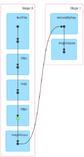
Figure 3: DAG representation for primary query, green dot represents caching point. ... 17
Figure 4: Time taken to first check the cache for given query, then if not in cache, desired data is retrieved as primary query (for each row) and analytical query is computed and saved in cache for future use... 19
Figure 5: Flow of RDDs ... 20
Figure 6: DAG representation for one body queries ... 21
Figure 7: Time taken to first check the cache for precomputed result for given query of center of mass... 22
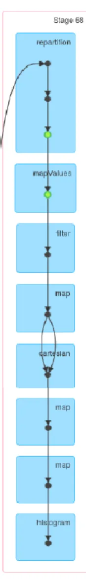
Figure 8: DAG representation of SDH computation using cartesian and repartition ... 24
Figure 9: Time taken to first check the cache for precomputed result... 25
Figure 10: DAG representation of SDH computation using groupByKey ... 25
Figure 11: Time taken to compute SDH using second approach and then display and store it in cache for future use. ... 26
Figure 12: Time taken to get the precomputed SDH result from cached parquet file. ... 28
Figure 13: Time taken to get the precomputed MOI result from cached parquet file. ... 28
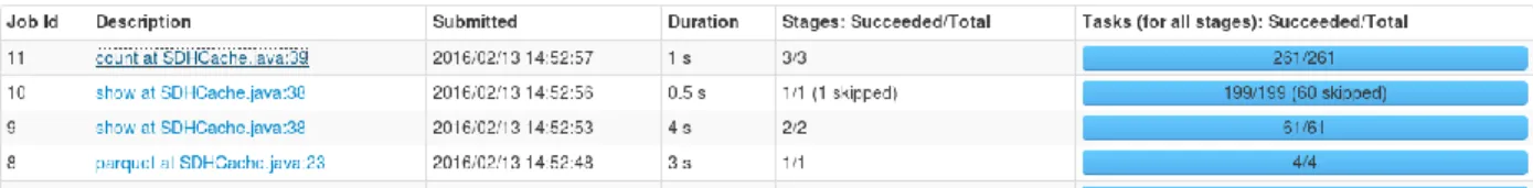
Figure 14: Time taken to fetch data and execute query and save the result. ... 29
Figure 15: The detailed view of job of query run in figure 14 in which main computation takes place... 29
Figure 16: Cached partition storing the data in the form of FrameAtomsRDD ... 30
Figure 17: Time taken to execute query to get moment of inertia and display and save result ... 30
iii
Figure 18: The detailed view of job of query run in figure 17 in which main computation
takes place... 30
Figure 19: Time taken to execute query to get SDH and display and save the result ... 30
Figure 20: The detailed view of job of query run in figure 19 in which main computation takes place... 31
Figure 21: Time taken to fetch the result of moment of inertia from parquet files ... 31
Figure 22: The detailed view of job of query run in figure 21 in which data is fetched ... 31
Figure 23: Time taken to fetch the result of SDH from parquet files ... 31
iv
ABSTRACT
Huge amount of data is being generated in almost every field and it cannot be avoided, rather is essential for the advancement of the field. Analysis of this data requires intensive computing power. Molecular Simulation is a powerful tool for understanding the behavior of natural systems. The simulation generates large amount data while observing the spatial and temporal relationships. The challenge is to handle the analytical queries that are often compute intensive.
Although various tools exist to tackle this problem, but in this paper we have tried an alternate approach that uses Apache Spark- a modern big data platform – to parallelize the computation of analytical queries. MsSpark consists of three layers: Apache Spark layer, MS RDD layer and MS Query Processing layer. MS RDD layers supports data that is specific to Molecular Simulation. MS Query Processing layer provides functionality of executing analytical queries. Caching is used to improve the performance. The system can be further extended to cover more analytical queries.
1
CHAPTER 1: INTRODUCTION
Substantial amount of data is being generated in virtually all fields from physics to genomics to social sciences. As the volume increases, the current solutions for data storage and processing show their limitations. The challenge is to provide the hardware architecture and corresponding software systems that could extract valuable knowledge from these large datasets. With the decreasing cost of memory, the storage of data is not a big deal nowadays. For data processing, map reduce is a trending programming model for processing large data sets with a parallel and distributed algorithm on a cluster. It provides efficient and fast solution for manipulation of large datasets.
Apache Spark is a fast in-memory data processing engine for batch, real-time and advanced analytics. It supports fast iterative data analyses on very large datasets. This paper presents an analytical tool, based on Apache Spark, built to process and extract knowledge from Molecular Simulation data. Molecular Simulation is a powerful tool for analyzing physical and chemical attributes of natural systems in the field of structural and molecular biology. These simulations generate data of natural particles such as atoms, molecules, etc. and presents the spatial and temporal relationship among them. The volume of data generated is massive which imposes serious challenges for data accessing, managing and analysis. A salient problem is the high computational complexity of analytical queries. This paper introduces MsSpark which is an in-memory cluster computing system for analyzing large volumes of Molecular Simulation data.
2
Spark revolves around the concept of a resilient distributed dataset (RDD), which is a fault-tolerant collection of objects partitioned across a cluster of machines that can be operated on in parallel. MsSpark provides support for Molecular Simulation data types and operations on top of the Apache Spark framework. The corresponding code can be found at
https://github.com/pkp927/MsSpark and it can be downloaded on the system with Spark installed and run on Molecular simulation data to execute queries. Till now, six queries have been
implemented: (1) Sum of Mass (2) Center of Mass (3) Moment of Inertia (4) Dipole Moment (5) Radius of Gyration (6) Spatial Distance Histogram (SDH). It can be extended further by
3
CHAPTER 2:
BACKGROUND AND RELATED WORK
A lot of work has been done in this field that resulted in existing systems that provide physicians and other interested users an interface to manipulate molecular simulations.
2.1 Molecular Simulation Analysis Tools
Molecular simulation data are used to study the features of biological system. Various tools have been developed to assist this process.
BioSimGrid [9] is a distributed database for Biomolecular simulations. It provides a database that stores data in three levels – Raw data, 1st level metadata that describes the generic properties of raw simulation data and 2nd level metadata that describes the generic level of simulation data. It allows software tools to be developed that can use the distributed database for interrogation and performing different analysis techniques across the range of different
trajectories. Basically, it is focused on the storage and access of molecular simulation data. It is still being worked on to focus on three key areas of simulation technology: high throughput simulation for high performance computing, a grid-enabled database for comparative analysis of simulation data, and multi-scale Biomolecular simulations ranging from the quantum-mechanical to the meso-scale.
SimDB [8] is another Grid software environment for Molecular Dynamics simulation and Analysis. Both Trajectory data and processed data are stored along with their metadata and user query is run by applying the filter function on the processed data. If it fails, then first processed data is generated from Trajectory data.
4
In BioSimGrid and SimDB [9-8], MS data are stored as raw flat files. Relational database is used for locating these files using metadata information. As sequentially scanning all the files is quite inefficient, so another tool known as Database Centric molecular simulation (DCMS) [7] has been developed that is built on top of relational database management system (RDBMS) providing an easy way to share, retrieve and analyze data without having to mess with raw data. Dynameonics [12] uses a similar approach as DCMS with concentrating on only protein data.
Molecular Dynamics Database MDDB [11] is also based on relational database. The framework uses a parallel and distributed PostgreSQL (Greenplum) for storing MD trajectory data and simulation job control information. It is under development and is focused on
exploration and analysis of simulations.
2.2 Spark Based Tools
Apache Spark is fast and general engine for large scale data processing. It has been leveraged as big data platform for many task applications.
Geospark [3] is a cluster computing framework for processing large scale spatial data. It extends the core of Apache Spark to support spatial data types, indexes and operations. It extends Spark with spatial RDDs (SRDDs) and introduces parallelized spatial transformations and
actions that provides an understandable interface for users to write spatial data analytics programs. It has three layers: Apache Spark layer, Spatial RDD layer and Spatial Query Processing layer.
Geotrellis is another project that adds GeoSpatial capabilities to Apache Spark. It is a geographic data processing engine for high performance applications. It uses Spark to work with raster data. Further, it has extension known as Geotrellis OSM Elevation which is a project that integrates OpenStreetMap data with Geotrellis to color the roads with elevation data.
5
Kira [5] is an astronomical image processing toolkit implemented with Apache Spark. Kira SE achieves a 3.7X speedup over an equivalent C program which indicates that Apache Spark are a performance alternative for many task scientific applications.
Influenced by above projects, we decided to implement Molecular Simulation queries using MsSpark which is based on Apache Spark. MS data is spatiotemporal in nature and is huge in amount. The processing of analytical queries involves high computational complexity. Hence, Apache Spark seems to offer an ideal environment for Molecular Simulation queries as is
6
CHAPTER 3: APACHE SPARK
Scientific analysis constitutes of tasks which are grouped into stages that are linked by various data flow patterns. The map-reduce model uses similar pattern to schedule jobs. The MapReduce programming model is clearly summarized in the following quote [1]:
“The computation takes a set of input key/value pairs, and produces a set of output key/value pairs. The user of the MapReduce library expresses the computation as two functions: map and reduce.
Map, written by the user, takes an input pair and produces a set of intermediate key/value pairs. The MapReduce library groups together all intermediate values associated with the same intermediate key I and passes them to the reduce function.
The reduce function, also written by the user, accepts an intermediate key I and a set of values for that key. It merges together these values to form a possibly smaller set of values. Typically just zero or one output value is produced per reduce invocation. The intermediate values are supplied to the user’s reduce function via an iterator. This allows us to handle lists of values that are too large to fit in memory.”
As clear from the above quote, the map-reduce systems consist of map stage and reduce stage which are linked by shuffle stage. No doubt, MapReduce greatly simplified “big data” analysis on large and unreliable clusters, but it has got its limitations. As the data is discharged to disk at the end of each map and reduce phase, traditional map-reduce platforms perform poorly on iterative and pipelined workflows. The map-reduce API has been criticized as inflexible.
7
Also, users wanted more complex, multi stage applications and more interactive queries that require efficient primitives for data sharing. And in MapReduce the only way to share data across jobs is stable storage. Therefore MapReduce is slow due to replication and disk i/o which are necessary for fault tolerance. In-memory data sharing can provide 10-100X faster systems.
To resolve these issues, Apache Spark has been developed which supports fast iterative data analyses on very large datasets. Apache Spark is an open source big data processing framework built around speed, ease of use, and sophisticated analytics. It was originally
developed in 2009 at UC Berkeley’s AMPLab, and open sourced in 2010 as an Apache project. It is a dataflow based execution system and has become extremely popular in industry and academic research groups in the analysis of large datasets. Spark improves over Hadoop
MapReduce with in-memory computing model that intrinsically supports iterative computation. Apache Spark is centered around Resilient Distributed Datasets (RDD) which is
distributed memory abstraction that allows in-memory computation on big data along with fault tolerance. RDD is the core concept in Spark framework. The main motivational factors behind the RDDs are iterative algorithms and interactive data mining tools that other computing frameworks handle inefficiently. Both these factors show impressive improvement in performance with in-memory system. RDDs use directed acyclic graph (DAG) to describe parallel tasks, provides fault recovery using lineage, lets user to explicitly persist intermediate results in memory, optimizes for data locality when scheduling work and manipulate them with rich set of operators.
Think about RDD as a table in a database. It can hold any type of data. Spark stores data in RDD on different partitions. To a programmer, they appear as an immutable collection of independent items distributed across a cluster of machines. An RDD can be stored in volatile
8
memory or persistent storage and can be converted to some other RDD through transformations. In Spark all work is expressed as either creating new RDDs, transforming existing RDDs, or calling operations on RDDs to compute a result. Each RDD is split into multiple partitions, which may be computed on different nodes of the cluster. So we can say that under the hood, Spark automatically distributes the data contained in RDDs across your cluster and parallelizes the operations you perform on them. RDDs can contain any type of Python, Java, or Scala objects, including user-defined classes.
RDDs leverage coarse grained transformations (e.g., map, filter, join) that apply same operation to multiple data items. This permits fault tolerance by logging the transformations (its lineage) rather than the data itself. If a partition is lost, then that partition of the RDD can be easily regenerated from other RDDs based on its lineage. Hence, lost data can be recovered without requiring costly replication. Also, because of lineage the RDDs do not need to be materialized all the times as it has enough information about how it was derived from other datasets to compute its partitions from data in stable storage.
Further, persistence and partitioning of RDDs can be controlled by the user. Users can choose RDDs that they will reuse along with the storage strategy. They can also specify an RDD to be partitioned based on a key that is useful for placement optimization.
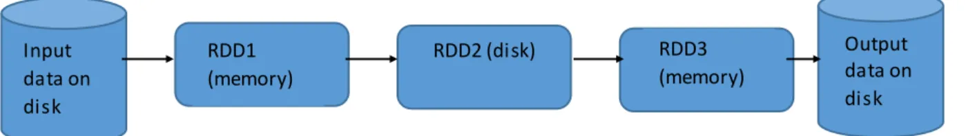
Figure 1: Data flow Input data on disk Output data on disk RDD1 (memory) RDD2 (disk) RDD3 (memory)
9
As observed in Figure 1, the data flow from one iteration to another happens through memory and does not touch the disk (except for RDD2). When the memory is not sufficient for the data to fit it, it can either be spilled to the drive or is just left to be recreated upon request for the same. Also, if different queries run on the same set of data again and again, this particular data can be kept in memory for better execution time.
Spark gives us a comprehensive, unified framework to manage big data processing
requirements with a variety of data sets that are diverse in nature (text data, graph data etc .) as well as the source of data (batch v. real-time streaming data). And you can use it interactively to query data
within the shell. In addition to Map and Reduce operations, it supports SQL queries, streaming data,
machine learning and graph data processing. Developers can use these capabilities stand-alone or combine them to run in a single data pipeline use case.
A Spark program consists of two programs: driver program and worker programs. Driver
program is written that implements the high level control flow of their application and launches various operations in parallel that run as worker programs on cluster nodes or as local threads. RDDs
are distributed across the workers.
Conclusively, the features of Apache Spark make it a compelling candidate distributed platform for analysis of dramatic dataset size.
10
CHAPTER 4:
MOLECULAR SIMULATION DATA
Molecular Simulation is a computational experiment conducted on molecular model. A molecular model postulates the interaction between the molecules and atoms. Molecular
Simulation is the only means to precisely determine the thermophysical properties of a molecular model system. These simulations are widely used for studying the behavior of biological systems as they provide a model description for biochemical and biophysical processes at the nanoscopic level.
In MS, the system of interest is a collection of a large number of natural particles such as atoms, molecules, etc. These natural particles interact under classical physics rule. Molecular Simulation generates large amounts of data as the system could consist of hundreds of thousands to millions of atoms. For example, a single snapshot of collagen fiber can consist of 890,000 particles. Also, one single simulation can run for tens of thousands of time steps. A single frame contains all the particles, together with all their measurements such as mass, charge, velocity, spatial coordinates, etc.
MS system typically generates output in the form of trajectory files containing a number of snapshots (frames) of the simulated system. Such data may be stored in binary form with some lossless compression. The format can be one of the MS file format e.g., GROMACS, PDB. This format is not recognizable, hence, needs to be translated into recognizable form. There are multiple files. The main file contains global data to identify the simulation and set of frames arranged sequentially. The main part in the frames data is the sequential list of each atom’s info
11
that includes its position, charge, mass, velocity, etc. The bond structure of the residue is stored in topology files and the control parameters are stored in the control file. For storage, this data is organized into directories. Data can be accessed either by encoding the description into the filenames or storing the description about the content in separate metadata files.
In this project, work is done on decompressed data which is in the following format: ATOM 00000000 00000004 00000001 17.808 15.749 6.649 -0.548 15.9994
1. First attribute is just telling whether it is an atom entry or a HEAD entry (there is only one HEAD entry per frame and it has some system property/information).
2. Second attribute is the frame number. 3. Third attribute is the atom ID/number. 4. Fourth attribute is the atom type.
5. Fifth, sixth and seventh attributes are the atom's position vector (x, y, z) . 6. Eight attribute is the atom's charge.
7. Ninth attribute is the atom's mass.
As Spark is flexible to work with data in various forms, it can be stored in various ways. It can be stored locally on the machine in compressed format and can be decompressed and fed to the Spark program.
HDFS can be used to store the data after decompressing it. HDFS is designed to reliably store very large files across machines in a large cluster. It stores each file as a sequence of blocks; all blocks in a file except the last block are the same size. The blocks of a file are replicated for fault tolerance. The block size and replication factor are configurable per file. An application can specify the number of replicas of a file. The replication factor can be configured
12
at file creation time and can be modified later. In HDFS, the files are write-once and have strictly one writer at any time.
As the size of decompressed data is quite large, it can be compressed to gzip format that is supported by Hadoop.
13
CHAPTER 5: ARCHITECTURE
The system consists of three layers.
5.1 Apache Spark Layer
It consists of regular operations supported by native Apache Spark which can be used to load and save data from/to storage.
5.2 MS RDD Layer
It extends the Spark with specialized RDDs that supports the Molecular Simulation data like FrameAtomsRDD and SelectedAtomsRDD and the output data like VectorRDD,
ScalarRDD, and HistogramRDD.
As the queries are frame specific, the input data is stored in pair RDD with the data of each atom in a frame paired with its frame number so that the queries can be performed based on the frame number. Various classes are created that support extraction of desired data from the raw data or other RDDs. Desired frames can be extracted directly from the raw file or from an RDD of previously extracted frames. Similarly, selection can be performed based on atoms. Desired atoms can be extracted directly from the raw file or from an RDD of previous extracted atoms.
Specific classes are also constructed to support operations on the Molecular Simulation objects. Each class facilitates working with data in a specific format. For example, Vector Class to facilitate calculating Moment of Inertia and Dipole Moment as these have three dimensions. Scalar Class to support one dimensional quantities.
14
Caching is also supported for each query. A separate class is defined for every query that supports the functionality of storing the generated results into the cache location and checking the cache location for stored result whenever new queries are asked.
5.3 MS Query Processing Layer
It supports Molecular Simulation Queries which are required to extract various statistical quantities out of data.
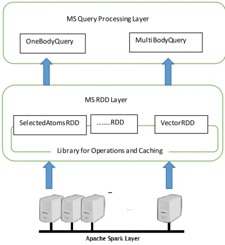
Figure 2: Architecture
First the desired data are extracted from raw data and cached in memory for different queries to run on it, so that it does not require to fetch same data again and again to compute different queries. The result of each of these queries is cached in parquet files from where it can
MS Query Processing Layer
OneBodyQuery MultiBodyQuery
MS RDD Layer
SelectedAtomsRDD …...RDD VectorRDD
15
be fetched easily for further statistical analysis. This way it reduces the computation of
calculating the result each time the query is asked by the user and lets the user ask these queries any number of times.
When the user invokes these queries, there are two possibilities (i) If it has not been computed before, then it is computed and stored as parquet file.(ii) If it has already been computed before, then it is directly accessed from the parquet files.
The functions defined in the Query Processing layer can be fetched by other application programs to perform the analytical queries. It can also be extended further to support more operations.
16
CHAPTER 6: PRIMARY QUERIES
Scientists need to enumerate various statistical quantities of MS data, which is
spatiotemporal in nature, in order to study the features of the natural system. MS data contain few numbers of physical features of numerous atoms present in the natural system recorded at tens of thousands of time steps in a single simulation. These features include position vector, charge and mass. Data of one time interval is called a frame. Therefore, MS data is a collection of data items which correspond to an atom in system at a particular time. Hence, each data item can be considered a point in multidimensional space.
To extract the statistical quantities from the data, analytical queries are executed against the data. These queries are mathematical function which translates a group of atoms to scalar, vector, matrix or data cube. These queries are run against a particular selection of data from the entire MS dataset. Thus, the processing of these queries requires two steps: (i) retrieve the group of desired atoms and (ii) compute the mathematical function.
For the first step, primary queries are used. Primary queries correspond to data selection queries that help to get information about a desired group of atoms captured by the simulation over which the analytical queries are run. They are necessary because mostly we are interested in a particular set of atoms or molecules and not the entire natural system. We want to compute statistical data of desired atoms to know their behavior in the natural system that was set up during the simulation.
17
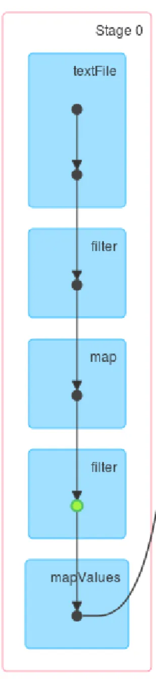
To maximize the performance in Spark, it is required to minimize the number of stages where a stage is a collection of tasks that can be done without shuffling of data. Spark actions are executed through a set of stages, separated by distributed “shuffle” operations. Primary queries are performed by four tasks that make up one stage.
18
Firstly, user is asked for selection parameters that includes a first frame number, last frame number, skip frame numbers, min, max, atom types and atom ids. First and last frame number tell the time frame we are interested in with skip frame numbers that include those frames which are in between the first and last frame that needs to be skipped, i.e., not considered. Min and max define the minimum and maximum position vectors of atom positions which represent the 3-D space in a frame of natural system that needs to be considered for calculation. Then atom types and atom ids identify the atoms that are required to be examined.
The file format is stored as an interface which is accessed to parse the data file. Broadcast variables are used to give a read only copy of file format indices and selection parameters to each node. Once the selection parameters are decided, transformations are applied to the raw data that is in the form of text file to create an RDD of selected atoms. SparkContext’s textfile method creates an RDD with each line as an element, so, first this method is used to create an RDD from the data file. Then filter transformation is used to get the atoms data only. With mapToPair transformation, pairRDD (key-value pairs) is created with frame number as key and an atom’s data as value. As there are many atoms in a single frame, therefore, there will be many key-value pair tuples corresponding to single frame number.
The resulting RDD named as SelectedAtomsRDD is a pairRDD with frame number as the key and atom information as double array value. This RDD can be partitioned in a way that each partition has single frame data using the method repartition passing the value of the number of frames as argument. Although repartition function results in the shuffle but it results in faster processing afterwards.
If more than one query is to be performed on the same selection of atoms, which happens usually, then the RDD can be cached for repeated use later without the need to fetch the desired
19
data from the raw file. It results in saving of a lot of time that is required to process the data retrieval queries again and again. Depending on the size of resultant SelectedAtomsRDD and available memory, the SelectedAtomsRDD is cached in memory or disk if memory is less. This diminishes the overhead of reading the raw data from disk.
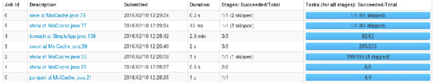
Figure 4: Time taken to first check the cache for given query, then if not in cache, desired data is retrieved as primary query (for each row) and analytical query is computed and saved in cache for future use. It shows about 2.9 min to retrieve desired data tested on 2GB raw data.
As the transformations are lazy in Apache Spark, hence they will not be materialized until an action is performed. So, SelectedAtomsRDD will not be materialized and cached until any action is performed on it which is carried out when performing analytical queries.
20
CHAPTER 7: ANALYTICAL QUERIES
For studying the statistical features of MS system, analytical queries are executed against the selected set of data from the entire simulation. Analytical queries are mathematical functions that map the recorded data of group of atoms to a scalar, vector, matrix or a data cube. These queries are workhorse tools for scientific discoveries. There are two types of analytical queries for MS system:
1. One-body queries are usually algebraic and involve attributes from a single atom. Each atom is processed a constant number of times, thus the total running time is O(n). These include moment of inertia, sum of mass, center of mass, radius of gyration, dipole moment, electron density, etc. Most of these queries is defined within a single frame. Only autocorrelation functions are defined on two frames.
2. Multi-body queries are holistic in nature and their computation involves more than one atom’s attribute. These include spatial density histogram (SDH) and radial density histogram (RDH).
Figure 5: Flow of RDDs
As the format of the result is either scalar, vector, matrix or data cube, so specialized VectorRDD, ScalarRDD, and HistogramRDD are defined to store the result of queries. The
RAW DATA FrameAtomsRDD/ SelectedAtomsRDD OneBodyQuery/ MultiBodyQuery VectorRDD/ ScalarRDD/ HistogramRDD
21
output can be stored in files for analyses. Following queries have been implemented in the system.
7.1 Moment of Inertia
Moment of Inertia is mass times the position vector and its result is in the form of 3D vector. It does not require any additional parameter. First using mapValues transformation, the information necessary to calculate the moment of inertia, i.e., mass and position vector is
extracted and multiplied for each atom from the SelectedAtomsRDD. Then, using reduceByKey action, summation is performed which produces the moment of inertia for each frame in the form of VectorRDD which is a pairRDD with frame number as key and corresponding moment of inertia value.
22
7.2 Sum of Mass
Sum of mass is the most basic function and it also does not require any additional parameter. First using mapValues transformation mass of each atom is extracted from
SelectedAtomsRDD. Then, using reduceByKey action, summation is performed which produces sum of mass for each frame in the form of ScalarRDD which is a pairRDD with frame number as the key and corresponding the sum of mass value.
7.3 Center of Mass
Center of Mass is moment of inertia divided by sum of mass and its result is in the form of 3D vector. It does not require any additional parameter. First using mapValues
transformation, the information necessary to calculate the moment of inertia, i.e., mass and position vector is extracted and multiplied for each atom and to calculate sum of mass, mass of each atom is extracted from the SelectedAtomsRDD. Then using reduceByKey action,
summation is performed which produces moment of inertia and the sum of mass for each frame. And finally, using mapValues transformation, moment of inertia is divided by sum of mass for each frame in the form of VectorRDD which is a pairRDD with frame number as the key and corresponding center of mass value.
Figure 7: Time taken to first check the cache for precomputed result for given query of center of mass. Then if not present in cache, center of mass is computed from the selected data that is cached in-memory while running primary query.
23
7.4 Dipole Moment
Dipole Moment is mass times the position vector and its result is in the form of 3D vector. It does not require any additional parameter. It is similar to the moment of inertia with charge in place of mass. First using mapValues transformation, the information necessary to calculate the moment of inertia, i.e., charge and position vector is extracted and multiplied for each atom from the SelectedAtomsRDD. Then using reduceByKey action, summation is
performed which produces a dipole moment for each frame in the form of VectorRDD which is a pairRDD with frame number as key and corresponding dipole moment value.
7.5 Radius of Gyration
Radius of Gyration is the square root of moment of inertia with respect to an axis divided by sum of mass. It has an additional parameter that defines the axis (x, y or z) with respect to which it is calculated. As usual, using mapValues transformation, the required information which includes mass and position with respect to a given axis multiplied together and mass individually is extracted from SelectedAtomsRDD. Then using reduceByKey action, summation is performed which produces moment of inertia and sum of mass for each frame. And finally, using
mapValues transformation, moment of inertia is divided by sum of mass for each frame and its square root is taken. The result is in the form of ScalarRDD which is a pairRDD with frame number as key and corresponding radius of gyration value.
7.6 Spatial Distance Histogram
Spatial Distance Histogram is one of the most common queries. It is a 2-body correlation function that computes distance between all pairs of points. It requires an additional parameter of bin width. There are various approaches to compute it. Two are discussed here.
24
One way is to first retrieve the location of all atoms using mapValues transformation. Then from the extracted data, locations are obtained frame wise and using cartesian and map transformations, all pairwise distances are calculated in each frame.
Then the histogram is created from the pairwise distances and stored in HistogramRDD which is a pairRDD that stores the frame number as key and corresponding histogram in the form of string as value. But this approach takes a lot of computational time as it extracts each frames data from the selected data and performs the operation framewise.
25
Figure 9: Time taken to first check the cache for precomputed result. Then if not present,
compute SDH using first approach and display and cache it for further use.
26
Another approach is to use groupByKey transformation to get a pairRDD of the frame number as key and locations of all atoms in that frame as value after retrieving the location of all atoms using mapValues transformation. Then using another mapValues transformation, the histogram is calculated for each frame in CalculateSDH class by finding the distance between all the pairs of atoms and computing histogram. It is stored in HistogramRDD which is a pairRDD that stores frame number as key and corresponding histogram in the form of string as value. This approach takes much less overall time than the first one.
Figure 11: Time taken to compute SDH using second approach and then display and store it in cache for future use.
27
CHAPTER 8: CACHING
As same queries on the same subset of data can be run many times by the user and they take large processing time, therefore, it is imperative to use caching to store already calculated queries in the form of DataFrames that is equivalent to tables in a relational database. Dataframes can be created from RDDs and structured data files. Dataframes are used to store the cached data as a parquet files. Parquet is a columnar format. Spark SQL provides support for creating Parquet files and data can be read and written into it while preserving the schema.
The schema has been defined for each type of query. Schema contains attributes for the selection parameters and the query result. The result is transformed to Dataframe with the defined schema and the Dataframe is stored as parquet file in the cache location which the user gives.
Whenever a query is asked, it is first checks in the cached location by extracting
Dataframe from parquet file and running SQL query on the Dataframe. If the query result is not present in the cache, then it is computed from the raw data and the result is stored in the cache for future access.
Also, while computing from the raw data, using the in-memory caching provided by spark, the intermediate data selection over which different analytical queries are to be run can be cached in memory so as to save time of retrieving the data selection again and again from the raw data. The primary queries are most time consuming because they involve data reads from disk. On the other hand, analytical queries are much less time consuming compared to primary
28
queries. So, it is imperative to cache the result of the primary queries in-memory for saving work of re-computing them.
Figure 12: Time taken to get the precomputed SDH result from cached parquet file.
29
CHAPTER 9: EXPERIMENTATION
The experiments to test the working of the application were run using Amazon EC2 which provides scalable deployment. 2GB raw data were used to run the queries. Raw data were stored on the cloud using Amazon Simple Storage Service. A cluster with 1 master node and 3 slave nodes was created. 18 GB memory (6 GB per node) was used.
First as the raw data is stored on S3, it takes time to fetch it from disk to memory in clusters. Hence the first query takes time as it involves fetching data from disk and persisting it in the form of FrameAtomsRDD on memory for future use.
Figure 14: Time taken to fetch data and execute query and save the result
Figure 15: The detailed view of job of query run in figure 14 in which main computation takes place.
30
Figure 16: Cached partition storing the data in the form of FrameAtomsRDD.
Once the data is in memory, further computations take less time to execute.
Figure 17: Time taken to execute query to get moment of inertia and display and save result.
Figure 18: The detailed view of job of query run in figure 17 in which main computation takes place.
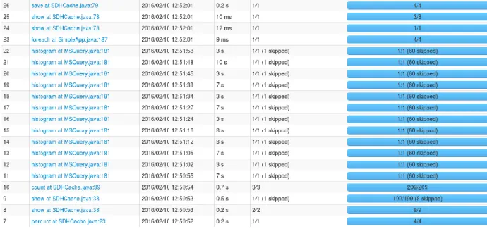
As SDH involves use of groupByKey transformation, therefore it is slow compared to one body queries.
31
Figure 20: The detailed view of job of query run in figure 19 in which main computation takes place.
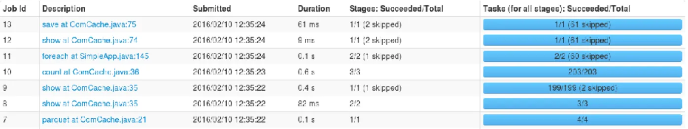
As the result of the queries run above are saved in parquet files, so when the application is run next time on same dataset with queries on the same subset, it fetches the result from parquet files rather than computing it from scratch.
Figure 21: Time taken to fetch the result of moment of inertia from parquet files.
Figure 22: The detailed view of job of query run in figure 21 in which data is fetched.
32
Figure 24: The detailed view of job of query run in figure 23 in which data is fetched.
As can be seen from the results, caching the result of the queries in the parquet files help in decreasing the computation time of multi body queries. It took 6 sec to compute the SDH and 0.2 sec to fetch the cached result from parquet files.
However, for one body queries, the computation time to execute the queries is less
compared to fetching it from parquet files which are stored on disks – S3. But it saves the time of fetching raw data from disk which is primary query that is necessary before running any
analytical queries. It takes 2.3 min to fetch raw data from disks (S3) to memory, whereas if the results were precomputed, it takes 2 sec to fetch the result from parquet files.
Due to Spark's in-memory computing, the computations on big data have become faster. However, primary queries involve starting from disks which is still slow. But if many queries need to be run then the one time fetch of raw data from disk can be compensated by the fast execution of analytical queries in memory.
33
CHAPTER 10: FUTURE WORK
This paper presents a solution to Molecular Simulation Analysis using the new trending domain, i.e. Apache Spark. It has laid the base for the development of full-fledged framework for processing large scale molecular simulation data. Currently, it processes data in decompressed form. The data generated by Molecular simulation are stored in the binary form with some lossless compression. The format can be one of the MS file format e.g., GROMACS, PDB. This format is not recognizable, hence, needs to be translated into recognizable form. So, first it is decompressed using the available tools and then the Spark application is run that accesses the decompressed data. As the decompressed data occupy huge amount of space, so it would be better if the data can be decompressed on the fly and fed to the Spark application to process it.
There are more options that can be opted for data storage. The present application can work with data stored either locally on disk or Hadoop Distributed File System but it has to be in the decompressed form. However, it is possible to decompress the data when needed and feed it to the application using pipes. For this few changes have to be made in the present application to use Spark Streaming which is an extension of the core Spark API that enables scalable, high-throughput, fault-tolerant stream processing of live data streams ingested from the sources like HDFS/S3, TCP sockets, etc. The processed data can then be pushed to filesystems, databases or live dashboards. Spark Streaming provides a high level abstraction called discretized stream or Dstream which is internally represented as a sequence of RDDS.
34
This paper concentrates on the processing of Molecular Simulation data to get results for the analytical queries and the ways to optimize them. It requires execution of primary and
analytical queries to get the final results. As discussed already, primary queries in which the data on which the analysis is to be performed is extracted from raw data, can be skipped if it’s already been computed and cached as intermediate RDDs. Then, the analytical queries are run and results are displayed and stored as parquet files for future use. The analytical queries can further be improved by implementing indexes that can be created on each partition after the intermediate RDDs creation and data partition.
As in Molecular Simulation system, data are queried using frame number and location of atoms, if a good spatial index that supports two dimensional data can be implemented to support three dimensional Molecular Simulation data then it can boost the performance of the system. There are various indexes like quad-tree and R-tree that have been implemented on spatial data using Apache Spark. As Molecular Simulation data is spatiotemporal in nature, so these indexes need to be modified to support 3rd dimension.
Till now, six Molecular Simulation queries have been implemented: (1) Sum of Mass, (2) Center of Mass, (3) Moment of Inertia, (4) Dipole Moment, (5) Radius of Gyration, (6) Spatial Distance Histogram. These are the most predominant queries. However, the system can easily be extended to support other Molecular Simulation analytical queries which are stated in Table 1. Further, user friendly interface can be implemented to make the user experience smooth.
35
REFERENCES
[1] Google’s MapReduce Programming Model Revisited - Ralf L¨ammel, Data Programmability Team, Microsoft Corp. Redmond, WA, USA
[2] Push-based System for Molecular Simulation Data Analysis - Vladimir Grupcev, Yi-Cheng Tu y, Joseph Fogarty, Sagar Pandit
[3] GeoSpark: A Cluster Computing Framework for Processing Large-Scale Spatial Data - Jia Yu, Jinxuan Wu, Mohamed Sarwat - School of Computing, Informatics, and Decision Systems Engineering, Arizona State University 699 S. Mill Avenue, Tempe, AZ
[4] Feig M, Abdullah M, Johnsson L, Pettitt BM (1999) Large scale distributed data repository: design of a molecular dynamics trajectory database. Future Generation Comput Syst 16(1):101–110
[5] Scientific Computing Meets Big Data Technology: An Astronomy Use Case - Zhao Zhang, Kyle Barbary, Frank Austin Nothaft, Evan Sparks, Oliver Zahny, Michael J. Franklin, David A. Patterson, Saul Perlmutter, AMPLab, University of California, Berkeley - Berkeley Institute for Data Science, University of California, Berkeley [6] Spark: Cluster Computing with Working Sets - Matei Zaharia, Mosharaf Chowdhury,
Michael J. Franklin, Scott Shenker, Ion Stoica - University of California, Berkeley [7] DCMS: A data analytics and management system for molecular simulation - Anand
Kumar, Vladimir Grupcev, Meryem Berrada, Joseph C Fogarty, Yi-Cheng Tu, Xingquan Zhu, Sagar A Pandit and Yuni Xia
[8] SimDB – A Grid Software Environment for Molecular Dynamics Simulation and Design: Design and User Interface – Matin Abdullah, Department of computer Science,
University of Houston
[9] BIOSIMGRID: A Distributed Database for Biomolecular Simulation, Bing Wu, Kaihsu Tai, Stuart Murdock, Muan Hong Ng, Steve Johnston, Hans Fangohr, Paul Jeffreys, Simon Cox, Jonathan Essex and Mark S.P. Sansom, Department of Biochemistry, University of Oxford, Science Centre, University of Oxford, Department of Chemistry, University of Southampton, Science Centre, University of Southampton
[10] Frenkel D, Smit B (2002) Understanding molecular simulation: from algorithm to applications. Computer Sci Ser 1. Academic Press
36
[11] Nutanong S, Carey N, Ahmad Y, Szalay AS, Woolf TB (2013) Adaptive exploration for large-scale protein analysis in the molecular dynamics database. In: Proceedings of 25th Intl. Conf. Scientific and Statistical Database Management. SSDBM. ACM, New York, NY, USA. pp 45–1454
[12] Van der Kamp M, Schaeffer R, Jonsson A, Scouras A, Simms A, Toofanny R,
Benson N, Anderson P, Merkley E, Rysavy S, Bromley D, Beck D, Daggett V (2010) Dynameomics: a comprehensive database of protein dynamics. Structure 18(4):423–435