THE APPLICATION OF COMPUTATIONAL MODELING TO DATA VISUALIZATION. Daniel S. Pineo.

(1)

THE APPLICATION OF COMPUTATIONAL MODELING

TO DATA VISUALIZATION

BY

Daniel S. Pineo.

B.S. University of Massachusetts, Amherst, MA (2000)

DISSERTATION

Submitted to the University of New Hampshire in partial fulfillment of

the requirements for the degree of

Doctor of Philosophy in

Computer Science

(2)

This dissertation has been examined and approved.

Dissertation Director, Colin Ware, Professor of Computer Science

David H. Laidlaw,

Professor of Computer Science

R. Daniel Bergeron,

Professor of Computer Science

Wheeler Ruml,

Assistant Professor of Computer Science

Kurt Schwehr,

Research Assistant Professor of Ocean Engineering

(3)

DEDICATION

(4)

ACKNOWLEDGEMENTS

I would like to foremost express my gratitude to my advisor, Colin Ware, for his guid-ance and support throughout my research. His invaluable insight focused me on what was important, and his imagination on what was possible. Many of the major ideas embodied in this work originated from discussions with him. This truly would not have been possible without him.

I would also like to thank my committee for their many valuable comments throughout the development of this work, and in particular David Laidlaw for providing the images used in his flow visualization evaluation paper.

Finally, I would like to thank my family. The encouragement, inspiration, and love of my wife, Gretchen, always gave me confidence and motivation when I needed it the most. I thank my parents, Carol and Craig, for their support and inspiration.

(5)

LIST OF FIGURES

1-1 The Three Pillars of Modern Science . . . 4

1-2 Scramjet CFD Model . . . 5

1-3 Andromeda CFD Model . . . 6

2-1 The Perception of Contours . . . 11

2-2 The Perceptual Enhancement and Inhibition of Edges . . . 12

2-3 The Early Human Visual System . . . 16

2-4 A Neuron . . . 17

2-5 V1 visual processing . . . 20

2-6 The Difference-of-Gaussians Receptive Field . . . 22

2-7 The Gabor Response Function . . . 24

3-1 Zhaoping’s Model of V1. . . 30

3-2 Regular Arrows . . . 38

3-3 Jittered Arrows . . . 39

3-4 Line Integral Convolution . . . 40

3-5 Aligned Streaklets . . . 42

3-6 Jittered Arrows Closeup . . . 43

3-7 Aligned Arrows Closeup . . . 44

3-8 Human Error Distribution . . . 46

3-9 Model Error Distribution . . . 47

3-10 Log Transformed Histogram . . . 47

(10)

4-1 The Neural Network Architecture . . . 56

4-2 V1 Gabor Kernels . . . 58

4-3 V1 Edge Enhancement Kernels . . . 59

4-4 Optimization Block Diagram . . . 63

4-5 Jobard & Lefer Visualization . . . 68

4-6 Optimized Flow Visualization . . . 68

4-7 Optimized Jet Stream Visualization . . . 69

4-8 Optimized Color Jet Stream Visualization . . . 69

4-9 Pixel Parameterized Visualization . . . 70

4-10 Line Integral Convolution Visualization . . . 70

4-11 Closeup of the discontinuities . . . 71

5-1 Node-link Diagram Example . . . 77

5-2 Layered Node-link Diagram Example . . . 78

5-3 Roelfsema’s Experiment . . . 80

5-4 Roelfsema’s Contour Tracing Operator . . . 82

5-5 Labeling in CortexSim . . . 83

5-6 Labeling Spread with Competitive Dynamics . . . 86

5-7 Two-layer Node-link Graph Diagram Example . . . 88

5-8 A Hermite spline . . . 89

5-9 The Link Tracing Experiment . . . 90

5-10 Model Iterations vs. Human Response Time . . . 92

5-11 Model Error vs. Human Error . . . 93

5-12 Sequence of Graph Optimizations . . . 94

5-13 Original vs. Optimized Response Time . . . 96

(11)

ABSTRACT

THE APPLICATION OF COMPUTATIONAL MODELING TO DATA VISUALIZATION

by

Daniel S. Pineo.

University of New Hampshire, December, 2010

Researchers have argued that perceptual issues are important in determining what makes an effective visualization, but generally only provide descriptive guidelines for transforming perceptual theory into practical designs. In order to bridge the gap between theory and practice in a more rigorous way, a computational model of the primary visual cortex is used to explore the perception of data visualizations.

A method is presented for automatically evaluating and optimizing data visualizations for an analytical task using a computational model of human vision. The method relies on a neural network simulation of early perceptual processing in the retina and visual cortex. The neural activity resulting from viewing an information visualization is simulated and evaluated to produce metrics of visualization effectiveness for analytical tasks. Visualization optimization is achieved by applying these effectiveness metrics as the utility function in a hill-climbing algorithm. This method is applied to the evaluation and optimization of two visualization types: 2D flow visualizations and node-link graph visualizations.

The computational perceptual model is applied to various visual representations of flow fields evaluated using the advection task of Laidlaw et al. [1]. The predictive power of the model is examined by comparing its performance to that of human subjects on the advection task using four flow visualization types. The results show the same overall pat-tern for humans and the model. In both cases, the best performance was obtained from visualizations containing aligned visual edges. Flow visualization optimization is done using

(12)

both streaklet-based and pixel-based visualization parameterizations. An emergent prop-erty of the streaklet-based optimization is head-to-tail streaklet alignment, the pixel-based parameterization results in a LIC-like result.

The model is also applied to node-link graph diagram visualizations for a node connec-tivity task using two-layer node-link diagrams. The model evaluation of node-link graph visualizations correlates with human performance, in terms of both accuracy and response time. Node-link graph visualizations are optimized using the perceptual model. The opti-mized node-link diagrams exhibit the aesthetic properties associated with good node-link diagram design, such as straight edges, minimal edge crossings, and maximimal crossing angles, and yields empirically better performance on the node connectivity task.

(13)

CHAPTER 1 INTRODUCTION

Perception is the means through which all data visualizations are processed, and the characteristics of successful data visualizations can often be traced back to percep-tual mechanisms of the human visual system. It is becoming increasingly recognized that the properties of human perception play a vital role in determining the effective-ness of data visualizations [2]. For example, the most successful flow visualizations contain contours tangential to the flow field. These visualizations take advantage of the edge detection mechanisms of human vision, which respond strongly to continuous contours. As a second example, visualizations that must convey fine spatial details are found to be more effective when they are rendered in greyscale then in a red-green scale or yellow-blue scale. This is because luminance contrast processing mechanisms of the visual system can convey far more detail than the chromatic contrast processing mechanisms.

1.1 Problem Statement

Despite the obvious relevance, perceptual theories have been of limited use to data vi-sualization designers because they are typically expressed in imprecise and descriptive forms that are not readily applicable. For example, the theory of contour perception states that two nearby visual objects that exhibit edges oriented close to the collinear axis between them will be perceived as a continuous contour [3]. While this theory suggests that we should limit our flow visualization designs to those with aligned

(14)

ar-rows, it still leaves and huge number of degrees of freedom unspecified. What about the myriad of other design choices? A data visualization designer would likely be interested in understanding the perceptual effects of the lengths of the arrows, the widths, their spacings, and the presence or lack of arrowheads. Certainly these all have some effect on the perceptual experience, but what is that effect? The space of possible visualization choices is enormous, and descriptive theories are not com-prehensive enough to describe it. As a result, creating effective data visualizations continues to be more of an art than a science.

Seminal flow visualization papers that introduced the most widely used flow visu-alization methods, such those of Cabral and Leedom [4], Jobard and Lefer[5], Turk and Banks [6], and van Wijk [7], give no indication of using perceptual theory in their development. Thus, there is clearly a gap between perceptual theory and its application to data visualization, which is likely due to the difficulty in applying such a descriptive theory in practice. In particular, computers are not capable of interpret-ing a descriptive theory, thus limitinterpret-ing their applicability. Interpretations by humans are often imprecise, inconsistent, and subjective.

Furthermore, these seminal flow papers lack psychophysical studies into the effec-tiveness of the visualization methods they introduce, although more recently Laidlaw et al. [1] conducted a study that showed large differences in the effectiveness of dif-ferent methods for a variety of visual tasks. Psychophysics complements perceptual theory, allowing designers to experimentally quantify the effectiveness of data visual-izations techniques by testing the performance of human test subjects on tasks requir-ing accurate interpretation of visualizations, but are often costly and time-consumrequir-ing. Laidlaw et al. only examined a tiny subset of the possible flow renderings, when all the parametric variations are considered. The combinatoric problem means that hu-man testing is not a viable technique for evaluating the space of design alternatives

(15)

for any reasonably complex visualization.

1.2 A Computational Approach

An alternative method of quantifying the effectiveness of a data visualization, one that addresses the shortcomings of descriptive theories and psychophysical tests, is highly desirable. What is needed is not just a perceptual theory, but a perceptual

computational model that allows data visualization designers to explore in detail how the perceptual mechanisms of the human visual system respond to a data visualiza-tion.

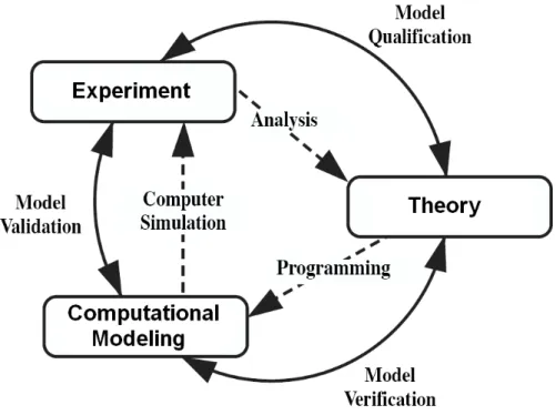
Computational modeling has now emerged as the third pillar of modern science (Figure 1-1), a peer alongside theory and physical experiment [8]. The basis for this claim is the enormous impact that computational modeling has had in the scientific disciplines where it has been successfully applied. Computational modeling has a history of tying together theory and experiment by showing how small scale mechanics produce large scale emergent behavior.

For example, computational modeling has become indispensable addition to the field of fluid dynamics. While closed form theories of fluid dynamics are capable of describing idealized systems, in even simple real world systems the behavior can quickly become too complex for them to be directly applied in practice. For exam-ple, the problem of designing of supersonic blunt nose aircraft confounded the fluid dynamics community throughout the 1950’s and early 1960’s [9]. The complexity of the mathematical analysis of this seemingly simple problem proved to be essentially intractable. Experimental approaches to fluid dynamics via wind tunnels have the limitations of being slow and expensive, and only yield a few variables such as lift and drag. These limitations have a striking resemblance to the current limitations of perceptual theory and psychophysical testing. In both cases, the theory is difficult

(16)

Figure 1-1: The three pillars of modern science: experiment, theory, and computa-tional modeling

to apply, with the experimental approach being slow, costly, and providing only a partial understanding of the system.

For the field of fluid dynamics, the solution to these problems arrived with the application of computational models. These computational fluid dynamics (CFD) models calculate the behavior of small units of volume each behaving according to the Naviar-Stokes equation (Figure 1-2), which describe the pressures and velocities of the fluid in the volume. The generalization afforded by this approach allows the model to be reused for arbitrary designs, there is no longer the need to create a new model for each design. The models allow designers to easily determine the pressures and velocities at any point. Thus, designers are able to inexpensively, interactively, and with great detail, explore the behavior of the system. Ultimately, the application of computational modeling profoundly changed the field of fluid dynamics.

(17)

ρ(∂v

∂t +v· ∇v) =−∇p+∇ ·T+f

Figure 1-2: The CFD model of the Hyper-X Scramjet that enabled NASA engineers to study its behavior while operating at Mach 7, the Naviar-Stokes equation on which the model is based [10].

Another example of the benefits of applying computational science can be found in cosmology. While the gravitational mechanics underlying the interaction of pairs of stars was well known, how these interactions produced the spirals and arms found in galaxies was an unsettled question. The number of stars involved was too large to be calculated analytically, and experimentation was clearly not possible. Finally, with the application of computational science, cosmologists were able to model galaxy behavior (Figure 1-3) and settle the question once and for all.

In many ways, data visualization designers find themselves in the same predica-ment. The complexity of real-world data visualizations interacting with the com-plexities of the human perceptual process makes the direct application of perceptual theories difficult. As with wind tunnels, psychophysical experiments allow the study of complex data visualization designs experimentally, but this approach is slow and

(18)

Figure 1-3: An N-body simulation of the Milky Way and Andromeda galaxy collision that will take place in 3 billion years [11].

expensive, and the data obtained for one design is not always generalizable to others. What data visualization designers lack is a computational model of perception anal-ogous to the CFD models that have benefited aeronautical designers. Such a model would not only provide a cheaper alternative to human psychophysical studies, but yield more detailed insight of the visual system’s response to those visualizations.

Computational models describe a system by calculating the behavior of a large number of simple, interacting elements. The complex behavior of the system emerges from the interaction of the simple elements. CFD models, for example, show how

(19)

complex behaviors such as waves, vorticies, and turbulence emerge from volume ele-ments (voxels) behaving according to the Naviar-Stokes formulas that describe fluid flow. For a computational neural model of visual perception, the simple elements are the neurons of the human visual system, and the emergent behaviors are the percep-tual mechanisms. There are many potential advantages to applying a computational modeling approach to data visualization:

• Simplicity - Computational models express complex behavior in terms of a few fundamental behavioral rules, enabling the behavior of the system to be more easily comprehended. By applying a computational model of visual perception to data visualization, a visualization practitioner could observe the effects that a visualization design have on the neural dynamics of the visual system, thus gaining insight into the reason for its effectiveness.

• Utility - Computational models produce numerical values that are suitable for use within a larger system. We explore this possibility in this thesis work by encompassing a computational model of perception within an optimization loop.

• Visibility - The numerical values with which computational models are ex-pressed afford the creation of visualizations that show the effects that the input design has on the model.

• Extensibility - Computational models can be easily integrated with other com-putational models. For example, a comcom-putational model of the early visual system might be integrated with a computational model of working memory, allowing designers to explore the cognitive load associated with a visualization.

• Generality - While descriptive models often describe very specific phenomena, a computational model of perception may be made to process arbitrary visual image inputs.

(20)

• Validation - The neural and psychophysical behavior predicted by computa-tional models can be compared with reality.

• Verification - A computational model provides a test of theoretical models. If the computational model yields the behavior predicted by the theoretical model, then this provides evidence that both the computational and the theoretical models are correct.

There are good reasons to believe that the ingredients are present for computa-tional modeling to make a similar contribution to the science of data visualization.

• The primary visual cortex (also known as area V1) of the brain contains a very large number of computational elements all performing the same task in parallel on different parts of an image. This means that high performance parallel processing can be applied.

• V1 has been extensively studied by vision researchers for several decades and its mechanisms are quite well understood.

• V1 is a critical area for pattern perception. It is here that the elements of form are processed. It is also here that the computations are made regarding which parts of an image will be visually salient. Although our understanding of the brain is too limited and computers are still insufficiently powerful to simulate the entire human brain we believe that useful progress can be made by simulating this critical brain area for visual processing.

1.3 Original Contributions

The contribution of this work is the application of the computational modeling paradigm to the problem of data visualization, and the demonstration that such

(21)

an approach can yield tangible results. Given the tremendous impact that computa-tional science has had on other scientific disciplines, it seems clear that exploring the viability of its application to data visualization is a worthwhile endeavor.

My contribution has five components:

1. Development of a computational model of human perception that simulates the visual mechanisms critical to the perception of data visualizations.

2. Comparison of the model evaluations with human performance on psychophys-ical tasks

3. Automatic optimization of data visualizations based on the effectiveness pre-dicted by the model.

4. Demonstration of the generality of the approach by the application to two dis-tinct classes of visualizations: 2D vector fields and node-link diagrams.

5. Establishment of computational modeling of perception as a “third pillar of science” in data visualization by developing its relationship with perceptual theory and psychophysical experimentation.

(22)

CHAPTER 2 BACKGROUND

The approach of using a perceptual model to optimize and evaluate data visualiza-tions as described in chapter 1 touches upon a diverse range of scientific disciplines, including data visualization, perception, neurophysiology, and computational model-ing. In this chapter, we review the relevant work within these fields as they pertain to this approach. In particular, we develop the relationship between these disciplines and how they relate to the end problem of data visualization.

2.1 Perception in Data Visualization

Perceptual theory is perhaps the most directly related to the field of data visualiza-tion, describing the visual mechanisms triggered when one views a data visualization. Such descriptions are useful for understanding the implications that the choice of visual variables has on the perception of a data visualization. Perceptual theory has been applied to a number of data visualization design problems, such as color sequences for color maps [12], node-link diagram layout [13] [14], symbol color and shape distinctiveness[15] , and texture coding for scalar maps [16].

2.1.1 Edge and Contour Perception

Of particular relevance to this thesis work is the perception of edges and contours in data visualizations. The flow visualizations and node-link graph diagrams that we model in this thesis work rely heavily on the use of edges and contours to convey

(23)

Figure 2-1: The perception of contours (from Field et al. [3]). The contour composed of aligned edges is easily perceived among a field of distractors.

information. Perceptual processing mechanisms enable a viewer to rapidly detect contours. Psychophysical research by Field et al. [3] has suggested that test subjects were able to identify a path of edge elements among a field of distractor elements (Figure 2-1). They found this to be reliable even as the elements were oriented up to 60◦ relative to each other. This suggests that there exists a perceptual mechanism in the visual system that is specialized in detecting continuous contours, and has given rise to the perceptual theory that two nearby visual objects that exhibit edges oriented close to the colinear axis between them will be perceived as a continuous contour.

(24)

Figure 2-2: The perceptual enhancement and inhibition of edges. The perception of nearby aligned edges are enhanced, while the perception of unaligned edges is inhibited. This mechanism enables continuous contours to be easily perceived.

This research on edge perception, along with neurophysiological evidence described later in section 2.3.4, suggests that there is some manner of lateral coupling among the visual elements involved in detecting the path of edge elements. They and other researchers have suggested that similarly oriented aligned contours mutually excite one another, whereas they inhibit other neurons that are nearby (Figure 2-2).

Ware [17] proposed that the effectiveness of flow visualizations can be linked to these perceptual processing mechanisms. Since conveying the path of flow advection is one of the primary goals of flow visualization, the most effective flow visualizations use contours to visually express the vector field. In effective flow visualization techniques, contours within the visualizations are evident and are tangential to the direction of flow. Laidlaw et al. [1] showed how to test the effectiveness of vector visualizations by tasking human subjects with estimating where the particle advecting within the flow field exits a bounding circle. They found that visualizations containing strong

(25)

perceptual contours along the flow direction tended to perform best.

The effectiveness of node-link graph diagrams can also be understood in terms of this contour perception mechanism. Node-link graph diagrams use visual contours connecting nodes to convey information. Smooth contours, lacking sharp angles or crossings, are perceived most readily by the visual system, and are thus most effective. This behavior is applied in data visualization in the form of graph layout aesthetics [18] [19], which provide guidelines for effective layout of node-link graph diagrams.

It is important to note, however, that perceptual theories of the kind discussed above are descriptive, rather than computational. As a result, they are capable of only providing general guidelines for data visualization design. Such descriptive theories cannot be used to quantitatively evaluate data visualizations.

2.2 Computational Models of Visual Perception

Applied to Data Visualization

In contrast to descriptive perceptual theories, computational models of perception enable the analytical evaluation of data visualizations. A significant advantage of such computational models is that they can be applied to a visual image using com-puter algorithms, unlike descriptive theories that require human interpretation. These models have been used to automatically evaluate the perceptual properties of visual popout, saliency, and clutter in data visualizations.

Visual popout is the mechanism of visual perception whereby conspicuous features in a visual scene can be easily found. Theories of popout suggest that visual features are processed in parallel to create a set of “feature maps” [20] [21]. Each feature map expresses the presence of some visual variable, such as size, orientation, or color, at all points in the visual space. Based on these theories, computational models of visual popout have been developed to predict the saliency of visual objects within a

(26)

scene [22], and such models have been applied to data visualization to predict how a viewer’s attention will be directed to relevant areas of a chart visualization [23] [24] [25].

Clutter is a concept closely related to visual popout, but describes factors that make targets harder, rather than easier, to see. Rosenholtz et al. [26] defined clutter as “the state in which excess items, or their representation or organization, lead to a degradation of performance at some task”, and offered two computational methods for measuring clutter.

The first method treats clutter from a purely information theoretic standpoint, by relating clutter to the number of bits required to encode the scene. While this method provides an elegant measure of clutter, it is not clear how this method relates to perceptual processes involved in the perception of clutter. The second method, which is based on a statistical measure of saliency, is more closely related to perceptual processing. This method calculates the ensemble of feature vectors in a scene. These feature vectors correspond to the local features detected in the early visual system, such as edges and color. The measure of clutter is derived from the volume of the feature space spanned by the ensemble. Both measures correlate well with human response time on search tasks using data visualizations, with no significant difference between the measures.

While these models seek to computationally express perceptual behavior when viewing data visualizations, they do not attempt to do so in a manner that is physi-ologically plausible. These models describe very specific perceptual behavior and are not straightforwardly extended to include additional behaviors. Nevertheless, this work represents the state of the art in applying models of perception to the problem of data visualization. Computational models based on the neurophysiology of the visual system have the potential to express not just one specific perceptual

(27)

behav-ior, but possibly many behaviors that may be relevant to the perception of a data visualization.

2.3 The Neurophysiology of Perception

Having argued the benefit of a computational neural model of perception for data visualization, and noting its potential for application in data visualization, we now review the architecture of the human visual system and explore the feasibility of con-structing a computational model that is capable of expressing the visual mechanisms observed in the perception of data visualizations.

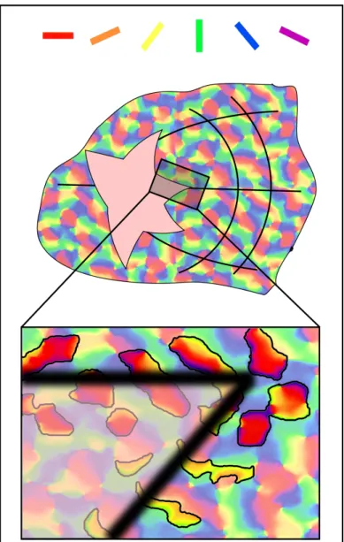
The early stages of the visual system are critical to the perceptual processing of data visualizations. When a visual image projects onto the retina at the back of the eye, receptors in the eye convert the image into electrical signals. These signals pass through the midbrain lateral geniculate nucleus (LGN), before proceeding to the pri-mary visual cortex (V1) at the posterior of the brain (Figure 2-3). These early stages of visual processing provide the foundation of pattern perception, color perception, texture and visual salience. Understanding how a visualization is processed in these stages can tell us a lot about how effective it will be. In the following brief review of relevant neurophysiology, we concentrate on aspects of the visual system that are relevant to the modeling effort. Specific neurophysiological measurements are given so they may be later incorporated into the computational model.

2.3.1 Neurons

The most basic building block of the visual system is the neuron. Neurons contain many branches, calleddendrites, that allow them to receive signals from other neurons (Figure 2-4). When a particular pattern of signals is received, the neuron may become excited and begin signaling other neurons along a branch called an axon. Neurons

(28)

Figure 2-3: The early stages of human vision. Light enters the eye and falls on the retina. Photoreceptors in the eye then send signals along the optic nerve, through the LGN, and finally to V1. The mapping of locations in the visual scene to neurons in V1 is depicted.

make on the order of 10,000 connections, calledsynapses, to other neurons. Depending on the neurotransmitter used by the neuron, its signals may have either excitatory or inhibitory effects on the recipient neuron. Signals from an excitatory neuron makes the neurons it signals more likely to become excited, and signals from inhibitory neurons make the neurons it signals less likely to become excited.

The current across the neural membrane was first expressed by Hodgkin and Hux-ley [28] as: I =CM dV dt + ¯gKn 4 (V −VK) + ¯gN am3h(V −VN a) + ¯gl(V −Vl)

whereI is the total current through the surface membrane of a neuron. It is dependent on both the conductivity of the synaptic connection and the activity of the source

(29)

Figure 2-4: An example of a neuron [27]. The neuron receives input signals along its dendrites, and sends an output signal along its axon.

neuron. In this equation, CMdV_dt is the capacitive current, ¯gKn4(V −VK) is an ionic

current of Potassium ions, ¯gN am3h(V −VN a) is an ionic current of Sodium ions, and

¯

gl(V −Vl) is a leakage current.

In artificial neural network models, the membrane conductances are often com-bined and simplified into a single weight parameter, wij. This parameter specifies the

ability of a signal to propagate from the presynaptic neuron i, to the postsynaptic neuron j. The overall activity of the postsynaptic neuron, yi, is then calculated with

the function [29]: yj =φ X i wijxi !

Where, xi is the activity of the presynaptic neuron, and φ is a sigmoid saturation

function. Thus, wij describes the pattern that the neuron responds to. In the early

visual system, these are localized visual patterns such as edges. The local visual area corresponding to the pattern is known as a receptive field.

(30)

2.3.2 The Eye and Retina

The visual image is projected by the lens of the eye and focused onto the retinal lining at the back of the eye. The light travels through the layers of the retina and falls upon the light-sensitive photoreceptor neurons. There exist approximately 6 million color-sensitive photoreceptors, known as cones, and approximately 100 million color-insensitive photoreceptors, known as rods. Cones are subtended by an angle of approximately .006 degrees and are the principle photoreceptors responsible for processing high-detail at normal light levels. Cones are most sensitive to a specific frequency of light, such as red, green, or blue, but all cones are capable of detecting white light. Thus, the retina is capable of processing black and white patterns at a higher level of detail than it can process blue-yellow or red-green patterns.

The signals produced by these photoreceptors are then processed by several layers of neurons in the retina. The receptive field surround signal is computed by horizontal [30] and amacrine cells that are connected laterally to nearby areas of the retina. Bipolar cells combine this surround signal with a center signal of an opposing polarity to produce what is known as a center-surround receptive field. Such a receptive field responds most strongly to light falling either in center of the field, or in the annulus surrounding center, but not both. Bipolar cells exist in both on-sensitive and off-sensitive forms, thus producing receptive fields that are off-sensitive to light in the center (on-center/off-surround) and as well as fields that are sensitive to light in the annulus (off-center/on-surround). Bipolar cells forward this signal to the retinal ganglion cells, which send the center surround signal along the optic nerve, through the lateral geniculate nucleus (LGN), and to the V1.

The central 2◦ of vision is processed by a 500µm diameter rod-free area of the retina known as the fovea [31]. It is this area that is responsible for processing fine detail. On average, there are approximately two retinal ganglion cells for each cone

(31)

in this area, one on-center and one off-center [32]. Away from the fovea, the cone spacing and the ratio of photoreceptors to retinal ganglion cells increases quickly, causing a drop in visual acuity in the periphery.

2.3.3 The Lateral Geniculate Nucleus (LGN)

The LGN is an area where the optic nerves from the two eyes connect in the mid-brain. It appears that one of the primary functions of the LGN is to physically reorganize the signal paths. For example, signals from the two eyes are brought into close proximity. Also, the signals from the rods and cones are separated so they may progress down different processing paths. The signal processing performed by LGN remains incompletely understood, but is believed to be involved in stereopsis. Be-cause this functionality is not pertinent to this work, the LGN is not included in the computational model.

2.3.4 V1

V1, also known as the primary visual cortex, is the first cortical processing area of vision, and is largely populated with neurons that are selective to orientated edges. These neurons are capable of detecting the edges of sinusoidal grating patterns with spatial frequencies up to 8 cycles per degree between 2◦ and 5◦ eccentricity [33], and presumably higher in the fovea. The receptive fields of V1 neurons are retinotopic, meaning that there is a direct mapping between a neuron’s location in V1 and it’s receptive field in visual space.

The architecture of V1 can best be understood in terms of columns and hyper-columns. A column is a cortical area of neurons that respond to a specific edge orientation and receptive field location [34] [35] and contains about 200 to 250 neu-rons [36]. These columns form a repeating pattern across the surface of V1, such that

(32)

Figure 2-5: The V1 visual processing of the scene from Figure 2-3. Red patches are cortical columns containing neurons that respond to horizontal edges, yellow patches are columns sensitive to edges angled at 60◦. Highlighted areas indicate columns that are active due to the edges of the star viewed in the visual scene.

within any 500µm diameter area columns all orientations are represented (Figure 2-5). Such an area is known as a hypercolumn. Both columns and hypercolumns lack well-defined borders in the visual cortex, however, their treatment as discrete, well-defined areas provides a useful approximation for understanding and modeling

(33)

cortical behavior.

Furthermore, there is evidence that the perception of an edge is enhanced by nearby edges with an aligned orientation [3]. Studies of the dendritic trees of V1 neurons suggest that this behavior is achieved via lateral connections, up to 4mm long, between neighboring columns in V1 [37]. V1 is notable for detecting visual feature dimensions including color, orientation, and simple motion, which form the basic primitives that are used in all subsequent processing. Higher level visual areas, such as V2 and V4, are currently not as well understood, and are not modeled in this work.

2.4 Neurophysiological Computational Models of Perception

The neurophysiology described in the previous section is responsible for the perceptual mechanisms activated when viewing data visualizations. By expressing this physiol-ogy in a computational form, we can construct a model that exhibits the behavior of the visual system, capable of being used to analyze data visualizations. In this section, we review mathematical models that have been used to describe aspects of the visual system.

2.4.1 Models of Retinal Center Surround Response

The center surround response of retinal ganglion cells can be described mathemati-cally using a Difference-of-Gaussians (DoG) function (Equation 2.1, Figure 2-6) [38]. This function contains a narrow excitatory center, produced by the cones of the retina and forwarded directly to the retinal ganglion cells by the bipolar cells. The excitatory center is encompassed by a larger inhibitory surround, produced by the inhibitory effect of nearby horizontal and amacrine cells.

(34)

Figure 2-6: The retinal ganglion Difference-of-Gaussians receptive field, containing an excitatory on-center (light) and an inhibitory off-surround (dark).

DoGx,y,σ1,σ2 =α1Gx,y,σ1 −α2Gx,y,σ2 (2.1)

Where Gx,y,σ denotes the normalized two-dimensional Gaussian kernel,

Gx,y,σ =

1 2πσ2e

−x2+y2

2σ2 _(2.2)

(35)

2.4.2 Models of V1 Edge Response

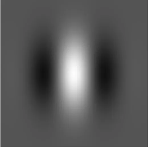
As noted in the previous section, the neurons of area V1 have been observed to respond preferentially to orientated edges [34] [35]. It has been argued that the Gabor function (Figure 2-7, Equation 2.3), defined mathematically as one-dimensional sinusoid encapsulated within a two-dimensional Gaussian envelope (Equation 2.2), is a good approximation for the edge patterns for which V1 neurons are selective [39]. Daugman argued that this function provides an optimal tradeoff between representing spatial position and frequency.

Gaborx,y,λ,σ,φ=Gx,y,σcos(

2π

λ x+φ) (2.3)

where λ defines the wavelength of the sinusoid, and φ defines the sinusoid offset.

2.4.3 Models of V1 Edge Enhancement

The edge enhancement behavior described in section 2.1.1 can be achieved by imple-menting the pattern of lateral excitation described in section 2.3.4. Such a model of V1 edge enhancement was developed by Zhaoping Li [40]. In this model, excitatory and inhibitory neurons exist in pairs, and together express the saliency of an edge. Li’s model focuses entirely on the contour enhancement mechanisms of V1. It does not include retinal processing, or even edge pattern recognition using a Gabor-like pattern matching elements. Thus, the model is not capable of processing an input image directly, but instead requires an array of edge perception strengths as input. The model uses a hexagonal array to represent the hypercolumn structure of V1, with each hexagon containing a set of 12 orientation selective columns. This model is described in more detail in chapter 3, where it is used as the basis for our model of flow visualization perception.

(36)

Figure 2-7: The Gabor response function, also with an excitatory center and inhibitory surround.

The LAMINART model is a more detailed and physiologically-based model of V1 edge perception developed by Grossberg et al. [41] [42]. It is considerably more detailed than Li’s model, including the center-surround processing of the retina and Gabor-like pattern matching of V1 neurons. The model also incorporates the individ-ual layers of neurons found in the neocortex, which are proposed to produce particular behaviors, including contour enhancement and convergence of neural activity. This model uses a regular grid layout and contains only two orientation selective columns per hypercolumn: vertical and horizontally selective columns.

(37)

many of the architectural feature found in the neocortex. From this model, Grossberg and colleagues demonstrated functionality such as contrast normalization, perceptual grouping [43] [44], texture segregation [45], and 3-D shape perception [46]. However, while these functionalities are of importance to a human’s ability to perceive data visualizations, the application of this model to the problem of data visualization has not been explored.

2.4.4 Models of Color Perception

While perhaps not as important as form perception for the visualization problems addressed in this thesis work, the perception of color is also relevant to data visu-alization design. The first stage of color processing by the cones of the retina can be modeled using the CIEL*a*b* [47] perceptual color space. The Hering opponent-process theory states that humans perceive color along white-black, red-green, and blue-yellow color dimensions. The CIEL*a*b* color appearance model describes this perceptual space using L*, a*, and b* coordinates, and defines the transformation to this color space from the standardized RGB space (sRGB). In the CIEL*a*b* space, the L* coordinate specifies the location of the color along the white-black dimension, a* specifies along the red-green dimension, and b* along the blue-yellow dimension.

2.5 Conclusion

These models demonstrate that is possible to neurophysiologically model the percep-tual mechanisms that play an important role in data visualizations. In this thesis work, we build upon these models to create a framework for computationally evalu-ating and optimizing data visualizations.

The work reviewed provides a powerful foundation for developing a computational modeling approach to data visualization. We’ve reviewed the relationships between

(38)

data visualization and perception, between perception and neurophysiology, and be-tween neurophysiology and computational modeling. These relationships transitively form an indirect relationship between data visualization and computational model-ing, and suggest computational modeling as a means of exploring the problem of data visualization. The goal of this thesis work is to explore the problem of data visualization in the context of this relationship with computational modeling.

(39)

CHAPTER 3 NEURAL MODELING OF FLOW RENDERING

EFFECTIVENESS

3.1 Introduction

Many techniques for 2D flow visualization have been developed and applied. These include grids of little arrows, still the most common for many applications, equally spaced streamlines [6] [5], and line integral convolution (LIC) [4]. But which is best and why? Laidlaw et al. [1] showed that the “which is best” question can be answered by means of user studies in which participants are asked to carry out tasks such as tracing advection pathways or finding critical points in the flow field. (Note: an advection pathway is the same as a streamline in a steady flow field.) Ware [17] proposed that the “why” question may be answered through the application of recent theories of the way contours in the environment are processed in the visual cortex of the brain. But Ware only provided a descriptive sketch with minimal detail and no formal expression. In the present chapter, we show, through a numerical model of neural processing in the cortex, how the theory predicts which methods will be best for an advection path tracing task.

Our basic rationale is as follows: tracing an advection pathway for a particle dropped in a flow field is a perceptual task that can be carried out with the aid of a visual representation of the flow. The task requires that an individual attempt to trace a continuous contour from some designated starting point in the flow until

(40)

some terminating condition is realized. This terminating condition might be the edge of the flow field or the crossing of some designated boundary. If we can produce a neurologically plausible model of contour perception then this may be the basis of a rigorous theory of flow visualization efficiency.

The mechanisms of contour perception have been studied by psychologists for at least 80 years, starting with the Gestalt psychologists. With advances in our knowledge of the physiology of the visual system, neurological theories of contour perception have begun to develop. In the present chapter, we show that a model of neural processing in the visual cortex can be used to predict which flow representation methods will be better. We apply the model to a set of 2D flow visualization methods that were previously studied by Laidlaw et al. [1]. This allows us to carry out a qualitative comparison between the model and how humans actually performed. We evaluated the model against human performance in an experiment in which humans and the model performed the same task.

This chapter is organized as follows. First we describe the CortexSim 1.0 model of visual perception used in this work. Next we show how the perceptual mechanisms of the model differentially process various flow rendering methods. Following this, we show how the model predicts different outcomes for an advection path tracing task based on Laidlaw et al.’s prior work. Finally we discuss how this work relates to other research that has applied perceptual modeling to data visualization and suggest other uses of the general method.

3.2 The Computational Model - CortexSim 1.0

The CortexSim 1.0 model of the visual system processes images in three stages. The first is an edge detection stage, which computes the visual edges in the scene. The second stage, which performs edge enhancement, calculates the enhancing effect that

(41)

aligned edges has on their detection. The final streamline tracing stage models the higher level cognitive process whereby a pathway is traced.

3.2.1 The Edge Detection Stage

CortexSim 1.0 computes visual edge detection using the Gabor model of V1 edge detection described section 2.4.2 and defined by equation 2.3. The input to this stage is a rasterized data visualization image. For parameters of the Gabor equation, we used φ = 0, causing the Gabor function to respond to lines in the center of the receptive field. We used λ = 21 pixels and σ = 7 pixels, producing a Gabor function where the center maximum and the two neighboring minimum are significant, but more distant maxima and minima become negligible. For γ we used a value of 1, resulting in a radially symmetric Gaussian envelope.

3.2.2 The Contour Enhancement Stage

The edge enhancement stage of the CortexSim 1.0 model is based on a neural model of V1 by Li [40], which deals with the neural interactions of V1 responsible for producing the perception of an extended contour from aligned visual edges. The detection of visual edges is not part of Li’s model, nor is the high-level perceptual process of streamline tracing. The CortexSim 1.0 model combines these components with Li’s V1 contour enhancement model.

Following Li’s model, CortexSim 1.0 uses a hexagonal array to represent the hyper-column structure of V1. Each hex contains a set of 12 orientation selective hyper-columns, oriented in 15-degree increments, and each column contains an excitatory and in-hibitory neuron, for a total of 24 neurons per hex. The signaling activity of neurons are modeled as floating point values.

(42)

Figure 3-1: Zhaoping’s Model of V1 [48]. Neurons with aligned receptive fields mutu-ally excite each other, and neurons with unaligned receptive fields inhibit each other.

enhanced or suppressed depending on the relative arrangement of their receptive fields. These lateral connections cause neurons with aligned receptive fields to interact such that they mutually excite each other. Similarly, neurons with unaligned receptive fields interact such that they mutually inhibit each other (Figure 3-1).

These dynamics are described as follows. The excitation of the excitatory neuron varies according to the equation:

(43)

d dtxiθ =−αxxiθ− X ∆θ Ψ(∆θ)gy(yi,θ+∆θ) +J0gx(xxθ) + X j6=i,θ Jiθ,jθgx(Xjθ) +Iiθ+I0 (3.1) The first term describes the voltage decay of the neuron’s value back to zero with a time constant of 1/αx, for which we use a value of 1. The second term inhibits edges of similar orientation mapping to the same receptive field. This is done by receiving inputs from the inhibitory neurons of the same receptive field and similar orientations. This behavior is produced by the Ψ function, defined by:

Ψ(θ) =                        1 if θ = 0 0.8 if |θ|= 15◦ 0.7 if |θ|= 30◦ 0 otherwise (3.2)

The activation functiongy defines the signal produced by an inhibitory neuron as

a function of voltage potential. Similarly, the functiongx defines the signal produced

by an excitatory neuron. It has the effect of clamping the excitatory signal to between 0 and 1. These functions are defined by:

gx(x) =                0 if x <1 x−1 if 1≤x≤2 1 if x >2 (3.3)

(44)

gy(y) =                0 if y <0 0.21∗y if 0≤y≤1.2 0.21∗1.2 + 2.5(y−1.2) if 1.2< y (3.4)

The third term is an excitatory neuron’s feedback to itself. J0 defines the strength of this feedback loop, for which we used a value of 0.8. The fourth term produces the edge enhancement; it models the excitatory signal to neighboring neurons that lie along the orientation direction in the manner depicted by figure 3-1. The function J defines the strength of the excitatory connection to a nearby neuron, and is defined by: Jiθ,jθ0 =                        0.126e−(β/d)2−2(β/d)7−d2/90 if 0< d≤10 and β < π/2.69 or 0< d≤10

and β < π/1.1 and|θ1|< π/5.9 and |θ2|> π/5.9 0 otherwise

(3.5)

Whereθ1 is the angle from the neuron’s orientation to the line connecting the two neurons, θ2 is the angle from the neighboring neuron to this line, β = 2|θ1|+ 2∗

sin(|θ1+θ2|), and d is the distance separating the neuron and its neighbor. Similarly, the function W defines the strength of the inhibitory connections from nearby neurons, and is defined by:

Wiθ,jθ0) =                0 ifd= 0 or d≥10 or β < π/11 or |∆θ| ≥π/3 or |θ1|< π/11.999 0.14(1−e−0.4(β/d)1.5 )e−(∆θ/(π/4)) _otherwise (3.6)

(45)

The fifth term is the input from the receptive field, calculated using the Gabor function described in the previous section. The sixth term describes a background signal that all excitatory neurons receive, and is set such that average neuron voltage in the network remains constant. The inhibitory neurons evolve by:

d

dtyiθ =−αyyiθ −gx(xiθ) +

X

j6=i,θ0

Wiθ,jθ0g_x(X_jθ0) +I_C (3.7)

Here the first term again acts to decay the value of the neuron back to zero. The second term is input from the excitatory neuron in the pair. The third term acts to inhibit edges that are of the same direction, but located orthogonally to the edge. This prevents multiple parallel edges from being produced. The last term is a background signal to all inhibitory neurons.

One of the main simplifications embodied in Li’s model of contour enhancement is that it fails to incorporate the way the mammalian visual systems scales with respect to the fovea. Real neural architectures have much smaller receptive fields near the fovea at the center of vision than at the edges of the visual field.

3.2.3 The Streamline Tracing Stage

Laidlaw et al. [1] compared the effectiveness of visualization techniques by presenting test subjects with the task of estimating where a particle placed in the center of a flow field would exit a circle. Six different flow field visualization methods were assessed by comparing the difference between the actual exit numerically calculated and the estimation of the exit by the human subjects. Laidlaw’s experiment was carried out on humans, but in our work we apply this evaluation technique to humans as well as to our model of the human visual system and use a streamline tracing algorithm to trace the path of the particle.

(46)

exist for people to judge a streamline pathway. We call it streamline tracing because the task requires the user to make a series of judgments, starting at the center, whereby the path of a particle dropped in the center is integrated in a stepwise pattern to the edge of the field. Though algorithms exist in the machine vision literature for contour tracing [49], we found these to be inappropriate for use in this application. Contour tracing algorithms are generally designed to trace out the boundary of a visual shape, but a streamline tracing algorithm must also be able to produce a streamline in a field of disconnected contours, such as is the case with the regular arrows. The streamline to be traced does not necessarily follow a visible contour, but instead be located between contours, and will sometimes pass through areas devoid of visual elements. Thus we developed a specialized algorithm that is capable of tracing streamlines that do not necessarily correspond to the boundary of any shape, but can pass between visual contours.

Perception utilizes a combination of top-down and bottom-up processes. Bottom-up processes are driven by information on the retina and are what is simulated by Li’s model [48]. Broadly speaking, top down processes reflect task demands and the bottom up processes reflect environmental information. Top-down processes are much more varied and are driven in the brain by activation from regions in the frontal and temporal cortex that are known to be involved in the control of pattern identification and attention [50]. All of the flow visualizations evaluated by Laidlaw et al. [1], except for LIC [4], contain symbolic information regarding the direction of flow along the contour elements (e.g., an arrowhead). In a perpetual/cognitive process this would be regarded as a top-down influence. At present our model does not deal with symbolic direction information, but it does do streamline tracing once set in the right general direction. In regards to streamline tracing, the bottom-up information is processed from the visual edges in the visualization, while the top-down information represents

(47)

the cognitive process of streamline pathway tracing.

Contour integration is modeled using the following iterative algorithm:

Algorithm 1 Contour Integration Algorithm current position ← center

current direction ← up

while current position is inside circledo

neighborhood ← all grid hexes within two hexes from current position

for all hex inneighborhood do for all neuron inhex do

convert neuron orientation to vector

scale vector byneuron excitation vector sum ← vector sum +vector

normalize vector sum

current position ← current position + vector sum current direction ←vector sum

end for end for end while

return current position

Algorithm 1 maintains a context that contains a current position and direction. Initially, the position is the center, and the direction is set to upward. This context models the higher-order, top-down influence on the algorithm that results from the task requirements (tracing from the center dot) and the directionality which in our experiment was set to be always in an upwardly trending direction.

(48)

the current position and moving the position a small distance (.5 hex radii) in that direction. The flow direction is calculated from the neural responses in the local neighborhood of the current position. The excitation of each neuron is used to gen-erate a vector whose length is proportional to the strength of the response and whose orientation is given by the receptive field orientation. Because receptive field orien-tations are ambiguous as to direction (for any vector aligned with the receptive field, its negative is similarly aligned). The algorithm chose the vector most closely corre-sponding to the vector computed on the previous iteration. Vectors are computed for all neurons in hypercolumns within a 2 hexes radius of the current position; they are summed and normalized to generate the next current direction.

Minor modifications changes were made from the method published by Pineo and Ware [51]. Previously, the algorithm considered only a single hex cell at each iteration of the algorithm. This causes undesirable behavior in some cases. For example, on visualizations with arrowheads, the neural network can yield a very strong edge orthogonal to the flow field positioned at the back of an arrowhead. If the algorithm considered only the edges at this point, it can deviate excessively from the correct path, despite the edges in nearby positions indicating the correct flow direction. Averaging over aneighborhood is more robust and representative of human visual processing, producing a stronger correlation with human performance.

3.3 Qualitative Evaluation

Four different flow visualization methods were used in our application of the com-putational model to flow visualization. We used our own implementations of four of the six flow visualization techniques used by Laidlaw et al. [1]. We investigated a regular arrow grid because gridded arrows are still the most commonly used flow visualization technique in practice. We also used grid of jittered arrows because of

(49)

the conjecture that jittering arrows improves perceptual aliasing problems [2]. We included Line Integral Convolution (LIC) [4] because of its widespread advocation by the visualization community [52] and head-to-tail aligned streaklets because of Laidlaw et al.’s finding that aligned streaklets produces the most accurate perception of advection pathway, and because of the theoretical arguments in support of this method [17]. Note that Laidlaw used Turk and Banks’ algorithm [6] to create aligned arrows on equally spaced streamlines whereas we used Jobard and Lefer’s [5] method to achieve the same effect without an arrowhead [53].

V1 is known to have detectors at different scales. However, to make the problem computationally tractable we chose only a single scale for the V1, and we compensated for this alteration by designing the data visualizations with elements scaled such that they were effectively detected by the Gabor filter used by the model. The widths of the arrows and streaklets were designed to be smaller than the central excitatory band of the Gabor filter. This permits the edge to be detected even if not precisely centered on the receptive field of the neuron. The spatial frequency of the LIC visualization is defined by the texture over which the vector field is convoluted. Our texture was created by generating a texture of random white noise of one-third the necessary size and scaling it up via interpolation. The resulting spacial frequency of the LIC visualization was of a scale that was effectively detected by the Gabor filters of the model.

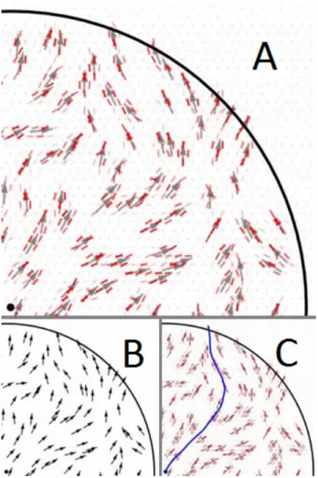
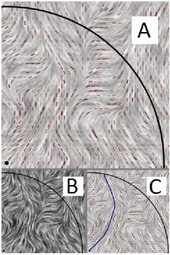
Samples of how the algorithm performed with the various visualization methods are shown in Figures 3-2, 3-3, 3-4, and 3-5. For greater clarity we only show a section of each image although the application of the algorithm to the whole image was computed. In each example the original visualization is shown in panel B, in the lower left. Panel A, in the top center, shows the effect of the Li algorithm on the image following ten feedback iterations, at which point the neural excitation values

(50)

Figure 3-2: Regular Arrows

had stabilized. The small bars show how strongly each neuron responds, with redder meaning stronger. Panel C, in the lower right, shows the path traced out by the contour integration algorithm.

Regular Arrows

The regular arrow visualization (Figure 3-2) is produced by placing arrow glyphs with uniform spacings. The magnitude of the vector field is indicated by the arrow length, and the flow direction by the arrow head. The grid underlying the regular arrows is apparent to humans, but the edge weights of the model show no obvious signs of being negatively impacted. In fact, the regularity ensures that the arrows are well

(51)

Figure 3-3: Jittered Arrows

spaced, thereby preventing any false edge responses produced by the interference of multiple arrows in close proximity. We expect that non-tangential edge responses will be produced by the arrowheads, leading to errors in the streamline advection tracing.

Jittered Arrows

The jittered arrow visualization (Figure 3-3) is derived from the regular arrows method, but the arrows are displaced a small random distance from the regular lo-cations. While composed of the same basic elements as the regular grid, we observe instances where nearby arrows interfere with each other and produce edge responses non-tangential to the flow direction. As with gridded arrows, the arrowheads excite

(52)

Figure 3-4: Line Integral Convolution

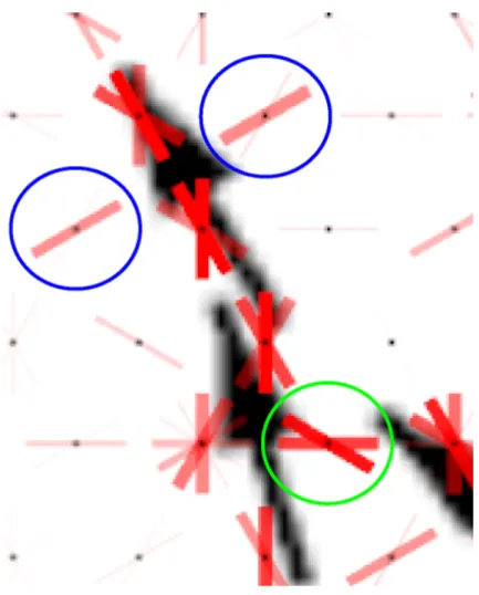
neurons with orientation selectivity non-tangential to the flow. This can be seen in Figure 3-6, where the back edge of the arrowhead causes orthogonal neural excitation to each side of the upper arrow (Figure 3-6, blue circles). We observe excitation resulting from the interference of two arrows at the bottom right (Figure 3-6, green circle). These non-tangential responses are much stronger than those found in the aligned streaklets visualization (Figure 3-7)

LIC

Line integral convolution (LIC, Figure 3-4) [4] images are formed by integrating a texture of random noise along the flow direction. The neurons of the model are not

(53)

strongly excited by the LIC visualization. Elongated patches of black or white produce the strongest responses, but these are still weak compared to other visualizations. However, we note the lack of responses that are not tangential to the flow direction. A major shortcoming of LIC is that it is completely ambiguous as to flow direction which could be in either of two directions at any point. In Laidlaw et al.’s experiment [1] this lead to very poor performance for LIC. However, because algorithm 1 did not take symbolic direction into account for any of the visualization methods (which we remedied with an upward bias as described in section 3.4.2), LIC could be expected to perform better in our experiment than it would in real-world practice.

Aligned Streaklets

In the aligned streaklets visualization (Figure 3-5), streaklets are aligned such that the head of one points to the tail of the next. This visualization produced strong neural responses within the model. As Ware argued [17], theory predicts that head to tail placement of arrows should produce good results. Perceptual theory suggests that evenly spaced streamlines should provide the best stimulus for coherent chains of excited neurons to develop.

3.4 Evaluation

By comparing the performance of humans to the model on the streamline advection task, we can attempt to understand in what cases the model adequately describes contour enhancement and extraction, and in what cases other perceptual mechanics may need to be incorporated. In order to compare how well the cortical model predicted human performance, we conducted an experiment where human subjects and the model completed the same task with the same set of flow representations. We chose Laidlaw’s streamline advection task [1].

(54)

Figure 3-5: Aligned Streaklets

3.4.1 Participants

Six human subjects were used in this experiment. They were a mix of volunteers and paid undergraduate students. There were four males and two females.

3.4.2 Vector Field Generation

Artificial flow fields were generated by interpolating a regular 8x8 grid of vectors. Each vector is a pseudo-randomly generated, normalized vector with a positive y component. This produced a vector field with an upward trend. This trend is im-portant for ensuring that all streamline paths eventually exit the circle. To vary the

(55)

Figure 3-6: Closeup of neural response to arrowheads. The black dots indicate the center of hypercolumns, red bars indicate the excitation of the orientation sensitive columns within the hypercolumn.

overall trending direction of the vector field, a pseudorandom angle was produced between 45◦, and all vectors were rotated by this value. The resulting vector fields thus trended in the upper 90◦ quadrant. This was motivated by the fact that the LIC method produces a visualization that is ambiguous; two possible flow directions may be inferred from any standard LIC image. In the experiment, we asked the subject to find pathways that trended upward. Likewise, the algorithm was also set to look for upwardly trending solutions.

(56)

Figure 3-7: Closeup of neural response to aligned streaklets

3.4.3 Instructions

Subjects were asked to click where they felt that a particle deposited in the middle of the circle would exit the circle. Due to the directional ambiguity of the LIC visualization, the subjects were informed that the general trend of the flow fields would always be upward.

3.4.4 Procedure

The subjects were presented with each flow field visualization on a 15.1 inch, 133dpi LCD screen. The diameter of the circle was 4.5 inches and the viewing distance

(57)

was approximately 57 cm. We evaluated four different visualization methods: regular arrows, jittered arrows, LIC, and aligned arrows. The test subjects were given as long as they needed to select with a mouse the point where they estimated that the particle in the center would exit the circle. Each test subject was first allowed to practice the task to minimize learning effects. Following this, they participated in 5 experiment blocks. Each block was constructed by generating 10 random flow fields and rendering them using the four visualization methods. The resulting 40 visualizations were then presented to the test subject in a random order. Following each block, the subjects were allowed to take a short break to minimize fatigue effects. Each test subject performed 200 tests, for a total of 1200 tests for the entire the experiment.

3.4.5 Computer Trials

The computer carried out exactly the same set of trials with exactly the same stimulus pattern generation algorithm. Raster images generated by the same four visualization methods were used as inputs.

3.5 Results

Figures 3-8 and 3-9 show histograms of the errors for the trials of the human par-ticipants and computer model, respectively. In both cases, most of the errors are less than three degrees. Because the error data were highly skewed we applied a log transform to the raw data before further analysis. This transform produced a roughly normal distribution (Figure 3-10), allowing the use of analysis of variance techniques. The geometric means for aggregated human performance and model performance are summarized in Figure 3-11. We conducted a two-way analysis of variance (ANOVA) with the two factors being aggregate human data and model output. ANOVA analysis revealed that the model was significantly more accurate than the human participants

(58)

Figure 3-8: Histogram showing distribution of errors for humans

[F(1,2966) = 128.22, p < 0.001]. The mean error of the CortexSim 1.0 model was .92 degrees, outperforming the human average of 1.5 degrees. There was no inter-action between the visualization type and whether the subject was the human or model. There was also a highly significant main effect for the type of visualization [F(3,2966) = 23.43, p < 0.001]. A Tukey HSD test indicated that the difference between LIC and aligned streaklets was not significant. However, there were signif-icant differences between all other visualizations. A linear fit of the error over the block number yielded that the block number was not significant on the human trials [F(1,1125) = 2.29, p = .13], indicating that fatigue and learning effects were not significant.

(59)

Figure 3-9: Histogram showing distribution of errors for the computer model

(60)

Figure 3-11: Mean errors for the four visualization methods for human participants and the model. Statistically distinguishable groups, with their performance rank or-dering, are indicated with orange boxes.

3.6 Discussion and Conclusion

The qualitative agreement between the results for human observers and the V1-based model provides strong support of the perceptual theory outlined in the introduction. The aligned arrows style of visualization produced clear chains of mutually reinforcing neurons along the flow path in the representation, making the flow pathway easy to trace as predicted by theory.

LIC produced results as good as the equally spaced streamlines, which lends sup-port to its popularity within the visualization community. While LIC did not produce as much neuron excitation as the aligned arrows method, this was offset by the lack of non-tangential edge responses produced by glyph-based visualizations. However, the relatively strong performance observed with the LIC visualization was achieved