Available at:
"Multi-input multi-output cost function for IFM-CAP model"
Henry de Frahan, Bruno ; Dong, Minh Giang ; De Blander, RembertAbstract
This rst part gives the main concepts for estimating a nested multi-input and multi-output cost function, preparing farm accounting data into input and output categories at dierent levels of aggregation and proceeding to the econometric estimation. These concepts will be implemented in the following parts of this project. With respect to previous work in that empirical domain, in particular the work as reported in Henry de Frahan et al. (2011) and De Blander et al. (2011), this work adds the original feature of introducing and implementing a cost function that is nested in an upper and a lower level of both input and output categories that allows to consider a wider range of input and output categories that is generally not considered in the available empirical literature on cost functions. The authors are not aware of previous development of a nested cost function in the literature while the concept of nested functions is widely used for production and utility functions. With respec...
Document type : Document de travail (Working Paper)
Référence bibliographique
Henry de Frahan, Bruno ; Dong, Minh Giang ; De Blander, Rembert. Multi-input multi-output cost function for IFM-CAP model. (2015) 111 p. pages
IFM-CAP model
Contract 153916-2013 A08-BE
Deliverable 8 : Final Report
Bruno Henry de Frahan, Jérémie Dong and Rembert De Blander
Earth and Life Institute, Université catholique de Louvain
I Design and Development
of a Method for Estimating Nested Cost and Input Demand
Functions
5
Introduction 6
1 Nested Cost and Input Demand Functions 7
1.1 Context . . . 7 1.2 The Nested Cost Function and its Derived Input Demand
Functions . . . 9 1.3 The Nested Input Demand Functions . . . 20 1.4 Conclusions . . . 29
2 Data and Aggregation 31
2.1 Introduction . . . 31 2.2 Data Preparation . . . 32 2.3 Aggregation Scheme . . . 33
II Design and Development
of a Method to Prepare and Update the Data from the
EU-FADN
39
Introduction 40
3 Törnqvist Index Construction 42
4 Imputation of Missing Prices 45
5 Output Data Preparation 48
MIMO Cost Function Estimation for IFM-CAP Model 153916-2013 A08-BE
5.2 Crop-specic Outputs . . . 52
5.3 Net Sale Value of Output Categories . . . 52
6 Input Data Preparation 55 6.1 Variable Inputs . . . 55
6.2 Fixed versus Variable Inputs . . . 58
6.3 Land . . . 60
6.4 Non-land Capital . . . 62
6.5 Estimation . . . 66
III Estimation of the Nested Cost
and Input Demand Functions for a Selection of Farm Types
and EU Regions
67
Introduction 68 7 Estimation Procedure 69 7.1 Preliminary Remark . . . 69 7.2 Cost Function . . . 69 7.3 System of Equations . . . 707.4 Symmetry and Adding-up Restrictions . . . 71
7.5 Monotonicity Conditions . . . 71
7.6 Curvature Conditions . . . 73
7.7 Estimation Method . . . 75
7.8 Rescaling the Output and Fixed Input quantities . . . 76
7.9 Further Remarks . . . 77
8 Selected Estimation Results 79 8.1 Introduction . . . 79
8.2 Estimated Cost Functions with Upper-level Inputs and Outputs for Crop Farms . . . 81
8.3 Estimated Cost functions with Upper-level Inputs and Lower-level Outputs for Crop Farms . . . 85
8.4 Estimated Expenditure Functions with Lower-level Inputs and Upper-level Outputs for Crop Farms . . . 90
8.5 Estimated Expenditure Functions with Lower-level Inputs and Outputs for Crop Farms . . . 93
IV Conclusions and Recommendations
98
Introduction 99
9 Main Challenges 100
9.1 Data Issues . . . 100
9.2 Aggregation of input and output categories . . . 101
9.3 Robustness of the Results . . . 101
9.4 Computational Requirements . . . 102
10 Strengths and Limitations 103 10.1 Main Strenghts . . . 103
10.2 Main Limitations . . . 104
11 Improvements 105 11.1 Removing Outliers . . . 105
11.2 Quasi-xed Input Allocation to Output Categories . . . 105
11.3 Alternative Functional Form . . . 106
Part I
Design and Development
of a Method for Estimating Nested
Cost and Input Demand Functions
This rst part gives the main concepts for estimating a nested multi-input and multi-output cost function, preparing farm accounting data into input and output categories at dierent levels of aggregation and proceeding to the econometric esti-mation. These concepts will be implemented in the following parts of this project. With respect to previous work in that empirical domain, in particular the work as reported in Henry de Frahan et al. (2011) and De Blander et al. (2011), this work adds the original feature of introducing and implementing a cost function that is nested in an upper and a lower level of both input and output categories that al-lows to consider a wider range of input and output categories that is generally not considered in the available empirical literature on cost functions. The authors are not aware of previous development of a nested cost function in the literature while the concept of nested functions is widely used for production and utility functions. With respect to this previous work, this work also calculates dierently land and non-land capital inputs, using a better estimate of the opportunity cost of capital as suggested in Andersen et al. (2011).
This nal report is organized in three parts, each one introducing the concept for estimating a nested multi-input and multi-output cost function, the concept for preparing farm accounting data into input and output categories at dierent levels of aggregation and the concept for proceeding to the econometric estimation.
Chapter 1
Concept for Estimating Nested Cost
and Input Demand Functions
1.1 Context
The overall objective of the project consists in developing and applying a method for estimating a theoretically consistent and exible multi-input multi-output cost function for a disaggregated set of input and output categories for individual FADN farms using EU-FADN data. The output categories need to be disaggregated at product level and the input categories at input level by farm type as reported in the EU-FADN data set.
The estimation of the theoretically consistent and exible input multi-output cost function reported in the FACEPA Deliverable 9.1 (De Blander et al., 2011) uses the Symmetric Generalized McFadden (SGM) functional form that is particularly ideal for applied work. Among the class of exible quadratic cost func-tions, the multi-input multi-output SGM cost function is a function for which the global curvature properties of a cost function can be imposed if needed without de-stroying its second-order exibility (see Diewert and Wales, 1987). It is expressed in terms of variable input prices, output quantities and quasi-xed input quanti-ties. The estimation also uses an augmentation of the SGM functional form to allow third-order terms in output quantities. This addition allows estimating cost functions for which marginal costs are downward sloping for some farms, a possible situation when outputs are limited by quotas. The estimation uses a medium-term and long-term versions of the SGM and augmented SGM functional forms. The estimates are obtained by a xed-eects non-linear seemingly unrelated regression (SUR) of input demands using an unbalanced panel of FADN farms from 1990 to the latest available year and imposing the theoretical restrictions on parameters, i.e.,
the symmetry and adding up restrictions, the curvature conditions of a theoretically consistent cost function, and/or the monotonicity conditions (see Chambers, 1988, p. 52 and 102). This SGM functional form is also used for estimating disagregated input demands because of its second-order exibility.
Because of limitations in degrees of freedom, risk of multicollinearity and failure to converge, the specication of cost function includes a limited number (three to ve) of variable input categories, a limited number (two to ve) of output categories and a limited number (one to three) of quasi-xed input categories by farm type. FACEPA Deliverable 9.2 (Bahta et al., 2011) reports a number of applications for crop, dairy and livestock farms for several representative EU regions and member states with convergence failures and unrealistic estimated marginal costs for some of the applications. IPTS would like to expand this theoretically consistent and exible multi-input multi-output cost function to a wider set of input and output categories at a more disaggregated level.
For that purpose, we will test a method to disaggregate the cost and input demand functions into a greater number of input and output categories relying on the concept of hierarchical or nested functions that is widely used in consumer demand analysis (Deaton and Muellbauer, 1999, p. 117-147), production analysis (Sato, 1967) and often applied in computable general equilibrium models. This concept rests on the assumption that a function of many arguments could be separate into sub-functions (see Green, 1964). The application of this concept to a cost function and its derived input demand functions assumes then the functional separability of broad output and input categories.
This separability assumption is acceptable to the extent that outputs sharing a similar underlying technology are grouped together in the same broad output cat-egory such that the technology of producing these outputs in one particular broad output category is separate from the technology of producing outputs belonging to another broad output category. This implies that producing one output belonging to a broad output category cannot directly aect producing another output that belongs to another broad output category. It can only aect indirectly producing this another output through producing the broad output category to which it be-longs. For instance, wheat and grain maize in one broad output category 'cereals' share the same technology while dry pulses and oil-seeds in another broad output category 'dry pulses & oilseeds' share another technology. Producing wheat cannot directly aect producing dry pulses through transformation eects, only indirectly if producing more wheat leads to producing more cereals and, hence, through trans-formation eects less dry pulses & oilseeds and, in turn, less dry pulses. If the
MIMO Cost Function Estimation for IFM-CAP Model 153916-2013 A08-BE marginal rate of transformation between two outputs in one broad output category is independent of any other output outside of that broad output category, then the production possibility function is said to be weakly separable in partition (Berndt and Christensen, 1973).
Similarly, this separability assumption is acceptable to the extent that inputs having a strong substitution among them are grouped together in the same broad in-put category such that inin-puts are similar in technico-economic characteristics within the same broad input category (Sato, 1967). This implies that the use of one input belonging to a broad input category cannot directly aect the use of another input that belongs to another broad input category. It can only aect indirectly the use of this another input through the use of the broad input category to which it belongs. For instance, wages and contract work in one broad input category 'services' are more similar in technico-economic characteristics than the broad input categories 'services' and 'other intermediate inputs'. Using contract work cannot directly af-fect the use of inputs belonging to the broad input category 'intermediate inputs' through substitution eects, only indirectly if using more contract work leads to using more services and, hence, through substitution eects less intermediate in-puts and, in turn, less inin-puts in that category. If the marginal rate of substitution between two inputs in one broad input category is independent of any other input outside of that broad input category, then the production function is said to be weakly separable in partition (Berndt and Christensen, 1973).
First, we describe the method for estimating a nested cost function and its de-rived input demand functions. Second, we describe the method for estimating nested conditional input demand functions. The description is done in generic terms to make it applicable to any specic situation of the FADN.
1.2 The Nested Cost Function and its Derived
In-put Demand Functions
The two-level cost function is proposed as an analogy to the two-level expenditure function proposed in the consumption theory (Deaton and Muellbauer, 1999, p. 117-147). The cost function has two levels: the lower level and the upper level. Assume that each broad output category m in the upper-level branch has an aggregate of
output sub-categories n in its lower level as subsets. First, we present the concept
for estimating the cost and input demand functions at the upper level of outputs. Second, we present the concept for estimating the cost and input demand functions at the lower level of outputs. These two concepts take inputs at their upper level.
In contrast to surveys on consumption expenditures that provide expenditures on specic consumption items, the EU-FADN data set does not provide disagregated total costs for specic output categories, neither the use of input categories for specic output categories. This project proposes and tests a method able to retrieve these missing disagregated farm data.
1.2.1 Cost Functions for Upper-Level Outputs
Let total variable cost for farmf at timet be represented by
T Cf t = T C(wf t, yf t, t;zf t;α) +ε0;f t, (1.1)
for y ≥ 0, with the usual theoretical properties (Chambers, 1988, p.52), where
wf t = (w1;f t, . . . , wJ;f t) represents the vector of broad input category prices, yf t = (y1;f t, . . . , yM;f t)the vector of broad output category quantities,zf t= (z1;f t, . . . , zK;f t)
the vector of quasi-xed broad input category quantities, and0;f t an error term
nor-mally distributed.
The dependent variable is obtained as
T Cf t = J
X
i=1
wi;f t·xi;f t.
where xf t = (x1;f t, . . . , xJ;f t) represents the vector of broad input category
quanti-ties.
Based on the cost function (1.1), cost minimization implies the following system of broad input demand equations
xi;f t = xi(wf t, yf t, t;zf t;α) +εi;f t (1.2)
wherei;f t represents an error term normally distributed.
By Shephard's lemma (Chambers, 1988, p.56),1 it holds that
xi(w, y, t;z;α) =
∂T C(w, y, t;z;α)
∂wi
,
forxi >0.
The system of broad input demand equations (1.2) is used to estimate the vector of parametersα. Estimated total costT Cd and estimated demands for a broad input
1As an important result of the envelope theorem, the Shephard's lemma states that, if the cost
function is dierentiable in input prices, then there exists a unique vector of cost-minimizing input demands that is equal to the gradient of the cost function in input prices.
MIMO Cost Function Estimation for IFM-CAP Model 153916-2013 A08-BE categoryxˆi are generated as
d T Cf t = T C(wf t, yf t, t;zf t; ˆα) ˆ xi,f t = xi(wf t, yf t, t;zf t; ˆα) (1.3) subject to y≥0 ˆ xi =xi(w, y, t;z; ˆα) if [(ˆxi >0) and (xi >0)] ˆ xi = 0 if not [(ˆxi >0) and (xi >0)] implying that d T Cf t ≥ J X i=1 wi;f t·xˆi;f t.
Leaving aside indexes f and t for clarity, the marginal cost function for broad
output category m is dened as
M Cm(w, y, t;z;α) =
∂T C(w, y, t;z;α)
∂ym
. (1.4)
Estimated marginal costs for a broad output category M Cd m are generated as d
M Cm;f t =M Cm;f t(wf t, yf t, t;zf t; ˆα).
From the cost function (1.1), it is then possible to obtain pseudo-observations of the total and average variable cost of broad output category m as the following.
Leaving aside indexes f and t for clarity, let us now, without loss of generality,
represent the estimated total cost functionT Cd as d T C(w, y, t;z; ˆα) = X m fm(ym) + X m X m0<m fm,m0(ym, ym0) +X m X m0<m X m00<m0 fm,m0,m00(ym, ym0, ym00) +. . .+f1,2,...,M(y1, . . . , yM), (1.5)
i.e., the sum of additive components, such that fm(ym) is only a function of one
output,fm,m0(ym, ym0)is a function of two outputs only, etc. Note that on the right
hand side all arguments except broad output category quantities y are omitted for
clarity.
time t, as2 d T Cm(w, y, t;z; ˆα) = fm(ym) + X m06=m τm;m,m0 ·fm,m0(ym, ym0) + X m06=m X m00<m0 τm;m,m0,m00 ·fm,m0,m00(ym, ym0, ym00) +. . .+τm;1,2,...,M ·f1,2,...,M(y1, . . . , yM), (1.6)
where the following cross-equation restrictions apply X k=m,m0 τk;m,m0 = 1, ∀m, m0;m0 6=m X k=m,m0,m00 τk;m,m0,m00 = 1, ∀m, m0, m00;m00 6=m0 6=m ... M X k=1 τk;1,2,...,M = 1, (1.7)
which ensure that
M
X
m=1
d
T Cm = T C.d
The coecientsτ distribute the non-additive terms of the estimated cost function
over the relevant broad output categoriesm. The above restrictions are fullled by
the following weights
τk;m,m0 = qk P k=m,m0qk , k=m, m0 τk;m,m0,m00 = qk P k=m,m0,m00qk , k=m, m0, m00 ... τk;1,2,...,M = qk PM k=1qk , k = 1, . . . , M (1.8)
2As an alternative, we could have dened the estimated total variable cost of output category
mat timet, keeping the other outputs at their observed level,
g T Cm(w, y, t;z; ˆα) = ym ˆ 0 d M Cm(w, y, t;z; ˆα) y m=u du.
However, sincedT C is not additively separable in outputsym, we have that d
T C 6= X
m g
MIMO Cost Function Estimation for IFM-CAP Model 153916-2013 A08-BE with natural candidates forqm being1,ym orfm(ym)if all such terms are present in
the estimated cost function (1.5). We choose the former to preserve the symmetry restrictions on cost functions.3
The average cost function for broad output category m can now be derived
straightforward
ACm(w, y, t;z;α) =
T Cm(w, y, t;z;α)
ym
. (1.9)
Pseudo-observations for the total variable cost of broad category output m are
now generated as
d
T Cm;f t = T Cm(wf t, yf t, t;zf t; ˆα). (1.10)
Pseudo-observations for the average variable cost of broad category output m
are now generated as d
ACm;f t = AC(wf t, yf t, t;zf t; ˆα). (1.11)
An empirical verication on preliminary results from estimations of total cost func-tions over a panel of Belgian crop, dairy and livestock farms (1990-2008) shows that the sum of the estimated total variable cost of output category m, i.e., T Cdm;f t, is equal to the estimated total variable cost, i.e., T Cdf t
d
T Cf t =PMm=1 T Cdm;f t. (1.12)
Note, however, that T Cm and ACm from (1.10) and (1.11) respectively are
c-titious total and average variable costs of broad output categorym since T Cm and
ACm are valid given that the other broad output categoriesm are at their observed
level.
Likewise, the marginal broad input demand function describes the amount of broad input categoryi that is allocated to broad output category m at the margin
3The symmetry restriction on cost functions imposesqmbe1to preserve such relationship (see
Section 7.4) ∂M Cdm ∂ym0 =∂M Cdm0 ∂ym ∀m, m0;m0 6=m.
of production (Beattie et al., 2009, p.132). It is given by mxi;m(w, y, t;z;α) = ∂xi(w, y, t;z;α) ∂ym (1.13) = ∂ 2T C(w, y, t;z;α) ∂ym∂wi = ∂M Cm(w, y, t;z;α) ∂wi .
Similarly as the estimated total cost function equation (1.5), leaving aside in-dexes f and t for clarity, represent the estimated input demand function xˆi as a
sum of additive components, such that gm(ym) is only a function of one output,
gm,m0(ym, ym0) is a function of two outputs only, etc. Proceding the same way, we
obtain the estimated demand for broad input category i that can be allocated to
broad output category m at timet, as expression (1.6)4
ˆ xi;m(w, y, t;z; ˆα) = gm(ym) + X m06=m τm;m,m0 ·gm,m0(ym, ym0) + X m06=m X m00<m0 τm;m,m0,m00·gm,m0,m00(ym, ym0, ym00) +. . .+τm;1,2,...,M ·g1,2,...,M(y1, . . . , yM), (1.14) subject to ˆ xi;m = ˆxi;m(w, y, t;z; ˆα) if (ˆxi;m >0) ˆ xi;m = 0 if not (ˆxi;m >0).
The coecients τ distribute the non-additive terms of the estimated input
de-mand function over the relevant broad output categoriesm using the same weights
as expressions (1.8) since it can be shown thatxˆi;m(w, y, t;z; ˆα)obtained from (1.14) 4As an alternative, we could have dened the estimated demand for broad input categoryithat
can be allocated to broad output categorymat timet, keeping the other outputs at their observed
level, e xi;m(w, y, t;z; ˆα) = ym ˆ 0 d mxi;m(w, y, t;z; ˆα)|ym=udu
However, sinceˆxi is not additively separable in outputsym, we have that
ˆ xi 6= X m e xi;m.
MIMO Cost Function Estimation for IFM-CAP Model 153916-2013 A08-BE or derived fromT Cdm(w, y, t;z; ˆα)(1.6) must have the same value.5
Pseudo-observations for the demand for broad input category i that can be
al-located to broad output categorym are generated as
ˆ
xi;m;f t = xi,m(wf t, yf t, t;zf t; ˆα). (1.15)
As expected, mixes of broad input categories xi;m per broad output category m
depend on relative prices of broad input category wi and the levels of the broad
output categories ym. These input mixes can be dierent depending on the broad
output category ym.
An empirical verication on preliminary results from estimations of total cost functions over a panel of Belgian crop, dairy and livestock farms (1990-2008) shows that the sum of the calculated demands for a broad input category i for a broad
output categorym, i.e.,xˆi;m;f t, is equal to the estimated total demand for that broad
inputi, i.e., xˆi;f t ˆ xi;f t = M X m=1 ˆ xi;m;f t (1.16)
at the condition that the following restrictions are removed
ˆ
xi;m = ˆxi;m(w, y, t;z; ˆα) if (ˆxi;m >0) ˆ
xi;m = 0 if not (ˆxi;m >0).
Again, note, however, that xi;m from (1.15) is a ctitious demand for a broad
input category i for a broad output category m since xi;m is valid given that the
other broad output categories m are at their observed level.
The cost for broad input category ithat can be allocated to broad output
cate-gorym is given by (wi·xi;m), which implies a predicted unit cost of
c
uci;m =
wi·xˆi;m
ym (1.17)
that varies according toym for a cost function that is non linear inym, and the total 5Note that the following comparative statics property of derived input demands is preserved
(Chambers, 1988, p.262) ∂xi;m ∂ym =∂M Cm ∂wi ∀i, m.
variable cost of broad output category m can also be predicted as d T Cm;f t = J X i=1 wi;f t·xˆi;m;f t. (1.18)
Note that it is possible to estimateT Cdm;f t either through (1.10) or (1.18).
1.2.2 Cost Functions for Lower-Level Outputs
Now, consider the vector of output sub-category quantitiesy˜m;f t = (ym,1;f t, . . . , ym,Nm;f t),
for which it holds that
ym;f t =
Nm
X
n=1
ym,n;f t
and assume that the estimated total variable cost of broad output category m is a
function of broad input category prices and of output sub-category quantities ym,n
using the separability assumption that the total cost function for one particular broad ouput category m does not depend on the level of the other broad output
categories m0 6=m
d
T Cm;f t = T Cm(wf t,y˜m;f t, t;zf t;βm) +η0;m;f t (1.19)
whereη0;m;f t represents an error term normally distributed.
Then, for each broad output category m, we derive the system of broad input
demand equations
ˆ
xi;m;f t=xi;m(wf t,y˜m;f t, t;zf t;βm) +ηi;m;f t (1.20)
whereηi;m;f trepresents an error term normally distributed and where, by Shephard's
lemma (Chambers, 1988, p.56), it holds that
xi;m(w,y˜m, t;z;βm) =
∂T Cm(w,y˜m, t;z;βm)
∂wi
forxˆi;m >0.
Estimation of βm proceeds as above using the values of the pseudo-observations ˆ
xi;m;f t from (1.15). Estimated total cost of the broad output category T Cddm and estimated demands for a broad input category for that broad output category ˆxˆ
i;m
MIMO Cost Function Estimation for IFM-CAP Model 153916-2013 A08-BE d d T Cm;f t = T Cm wf t, yf t, t;zf t; ˆβm ˆ ˆ xi;m;f t = xi;m wf t, yf t, t;zf t; ˆβm (1.21) subject to ˆˆ xi;m = ˆxi,m w, y, t;z; ˆβm if (hxˆˆi;m >0) and (ˆxi;m >0) i ˆ ˆ xi;m = 0 if not [(ˆxˆi;m >0) and (ˆxi;m >0))] implying that d d T Cm;f t ≥ J X i=1 wi;f t·ˆxˆi;m;f t.
If needed, the marginal cost M Cm,n as in expression (1.4), the total variable
cost T Cdm,n as in expression (1.6) and the average cost ACm,n as in expression (1.9) functions for output sub-category m, n of broad output category m can be
dened as above. The same verications on consistency between the aggregate and disaggregate quantities apply also here
d d T Cm;f,t = Nm X n=1 d T Cm,n;f t where d d T Cm;f,t=T Cm wf t,y˜m;f t, t;zf t; ˆβm .
Again, the marginal broad input demand function describes the amount of broad input category i that is allocated to output sub-category m, n of broad output
categorym at the margin of production. It is given by mxi;m,n(w,y˜m, t;z;βm) = ∂xi;m(w,y˜m, t;z;βm) ∂ym,n (1.22) = ∂ 2T C m(w,y˜m, t;z;βm) ∂ym,n∂wi = ∂M Cm,n(w,y˜m, t;z;βm) ∂wi .
Similarly as the estimated total cost function equation (1.5), represent the es-timated input demand function ˆxˆ
i;m as a sum of additive components, such that
gm,n(ym,n)is only a function of one output,gmn,mn0(ym,n, ym,n0)is a function of two
outputs only, etc. Proceding the same way, we obtain the estimated demand for broad input categoryithat can be allocated to output sub-category m, nat time t,
as expression (1.6)6 ˆ xi;m,n w,y˜m, t;z; ˆβm = gm,n(ym,n) + X n06=n τm,n;mn,mn0 ·gm,n;m,n0(ym,n, ym,n0) + X n06=n X n00<n0 τm,n;mn,mn0,mn00·gm,n;m,n0;m,n00(ym,n, ym,n0, ym,n00) +. . .+τm,n;m1,m2,...,mN ·gm,1;m,2,...;m,N(ym,1, . . . , ym,N)(1.23), subject to ˆ xi;m,n = ˆxi;m,n w,y˜m, t;z; ˆβm if (ˆxi;m,n >0) ˆ xi;m,n = 0 if not (ˆxi;m,n >0).
The coecients τ distribute the non-additive terms of the estimated input
de-mand function over the relevant output sub-categoriesm, n using the same weights
as expressions (1.8) but qm,n being 1, ym,n orgm,n(ym,n) since it can be shown that ˆ
xi;m,n
w,y˜m, t;z; ˆβm
obtained from 1.23 or derived from T Cdm,n
w,y˜m, t;z; ˆβm
must have the same value.7
Pseudo-observations for the demand for broad input category i that can be
al-located to output sub-categorym, n are generated as
ˆ xi;m,n;f t = xi;m,n wf t,y˜m;f t, t;zf t; ˆβm . (1.24)
As expected, mixes of estimated broad input categories xi;m,n per output
sub-category m, n depend on relative prices of broad input category wi and the levels 6As an alternative, we could have dened the estimated demand for broad input categoryithat
can be allocated to output sub-categorym, nat timet, keeping the other outputs at their observed
level, e xi;m,n w,y˜m, t;z; ˆβm = yˆm,n 0 d mxi;m,n w,y˜m, t;z; ˆβm y m,n=u du
However, sinceˆxi,m is not additively separable in outputsym,n, we have that
ˆ xi;m 6= X n e xi;m,n.
7Note that the following comparative statics property of derived input demands is preserved
(Chambers, 1988, p.262) ∂xi;m,n ∂ym,n =∂M Cm,n ∂wi ∀i, m, n.
MIMO Cost Function Estimation for IFM-CAP Model 153916-2013 A08-BE of the output sub-categories ym,n. These input mixes can be dierent depending on
the output sub-categoryym,n.
The same verications on consistency between the aggregate and disaggregate quantities apply also here
ˆ ˆ xi,m;f t = Nm X n=1 ˆ xi;m,n;f t
at the condition that the following restrictions are removed
ˆ xi;m,n = ˆxi;m,n w,y˜m, t;z; ˆβm if (ˆxi;m,n >0) ˆ xi;m,n = 0 if not (ˆxi;m,n >0).
Again, note, however, thatxˆi;m,n from (1.24) is a ctitious demand for a broad input
categoryi for an output sub-category m, nsince xˆi;m,n is valid given that the other
output sub-categoriesm, n are at their observed level.
The cost for broad input categoryithat can be allocated to output sub-category m, nis given by (wi·xi;m,n), which implies a predicted unit cost of
c
uci;m,n =
wi·xˆi;m,n
ym,n (1.25)
that varies according to ym,n for a cost function that is non linear in ym,n, and the
total variable cost of output sub-categorym, n can also be predicted as
d T Cm,n;f t = J X i=1 wi;f t·xˆi;m,n;f t. (1.26)
1.2.3 A Remark about Theoretical Consistency between Cost
Functions
Deneyf t = (˜y1;f t, . . . ,y˜M;f t), then total variable cost can be written as8
T Cf t = T C
wf t,yf t, t;zf t;α
. (1.27)
Then, which restrictions does our procedure impose on T C(w,y, t;z;α)? Are
the marginal cost functions M Cm,n(w,y, t;z;αˆ) of this total cost identical to the
ones obtained by our nested procedure? In other words, given T C(w, y, t;z;α)
and T Cm(w,y˜m, t;z;βm), what does T C(w,y, t;z;α) looks like and is it an ac-8Bold letters are used to distinguish the function, variables and parameteres of expression (1.27)
ceptable form for a cost function? The dierence is that T C(w, y, t;z;α) and
T Cm(w,y˜m, t;z;βm)are more restrictive thanT C(w,y, t;z;α)considering the
func-tional separability of the broad output categories that is embedded.
1.3 The Nested Input Demand Functions
The two-level production function was proposed by Sato (1967). The production function has two levels: the lower level and the upper level. Assume that each broad input categoryi in the upper-level branch has an aggregate of input sub-categories i, j in its lower level as subsets. First, we present the concept for estimating the
input demand functions in its lower level conditional to the upper level of input. It is then possible to calculate the demands for input sub-categories i, j and broad
output category m and, similarly, the demands for input sub-categories i, j and
output sub-category m, n. Note that the estimation of the nested conditional input
demand functions has no implication on the estimation of the nested cost functions.
1.3.1 Demand Functions for Lower-Level Inputs
Consider the vector of input sub-category quantities x˜i;f t = (xi,1;f t, . . . , xi,Ji;f t) and
the vector of input sub-category pricesw˜i;f t = (wi,1;f t, . . . , wi,Ji;f t), for which it holds
that
xi;f t = PJj=1i xi,j;f t
Ei;f t = PjJ=1i wi,j;f t·xi,j;f t
Expenditure minimizationEion the use of input sub-category quantities(xi,1;f t, . . . , xi,Ji;f t)
subject to input sub-category price levels (wi,1;f t, . . . , wi,Ji;f t) and an broad input
category quantity level xi;f t that is function of xi;f t(xi,1;f t, . . . , xi,Ji;f t, t) as in Sato
(1967)9 implies the following system of input sub-category equations for each broad input categoryi
xi,j;f t =xi,j( ˜wi;f t, xi;f t, t;γi) +µi,j;f t (1.28)
where µi,j;f t represents an error term normally distributed, and the corresponding
indirect expenditure function on broad input category xi;f t
Ei;f t=Ei( ˜wi;f t, xi;f t, t;γi) +µ0;i;f t (1.29) 9Sato (1967) uses a constant elasticity substitution (CES) form.
MIMO Cost Function Estimation for IFM-CAP Model 153916-2013 A08-BE
forxi,f t ≥0, whereµ0;i;f t represents an error term normally distributed.
By Shephard's lemma, it holds that
xi,j( ˜wi, xi, t;γi) =
∂Ei( ˜wi, xi, t;γi)
∂wi,j
forxi,j >0.
The system of conditional input sub-category demand equations (1.28) is used to estimate the vector of parameters γi. Estimated expenditure for a broad input
categoryEbi and estimated demands for input sub-category xˆi,j are generated as b Ei;f t = Ei( ˜wi;f t, xi;f t, t; ˆγi) ˆ xi,j;f t = xi,j( ˜wi;f t, xi;f t, t; ˆγi) (1.30) subject to xi ≥0 ˆ
xi,j =xi,j( ˜wi, xi, t; ˆγi) if [(ˆxi,j >0) and (xi,j >0)] ˆ
xi,j = 0 if not [(ˆxi,j >0) and (xi,j >0)]
implying that b Ei,f t≥ J X j=1 wi,j;f t·xˆi,j;f t.
As expected, mixes of estimated sub-category inputs xˆi,j depend on relative
sub-category input priceswi,j and the level of the broad input categoryxi, which depends
in turn on the levels of broad output categories ym.
Note that Ji X j=1 ˆ xi,j;f t 6= ˆxi;f t but Ji X j=1 (ˆxi,j;f t+µi,j;f t) = ˆxi;f t+εi;f t since Ji X j=1 xi,j;f t=xi;f t.
broad input category i is dened here as M Ei( ˜wi, xi, t;γi) =
∂Ei( ˜wi, xi, t;γi)
∂xi
. (1.31)
Estimated marginal expenditures for a broad input categoryM Edi are generated as
d
M Ei;f t=M Ei;f t( ˜wi;f t, xi;f t, t; ˆγi).
The average expenditure function for broad input categoryi is dened as AEi( ˜wi, xi, t;γi) =
Ei( ˜wi, xi, t;γi)
xi
. (1.32)
Estimated average expenditures for a broad input category AEdi are generated as
d
AEi;f t=AE( ˜wi;f t, xi;f t, t; ˆγi).
1.3.2 Demand Functions of Lower-Level Inputs for
Upper-Level Outputs
From the estimated input demand function (1.30), it is then possible to obtain pseudo-observations for the demand for input sub-categoryi, j that can be allocated
to broad output category m as the following. But, rst dene this new predicted
estimated demand function for input sub-categoryi, j as10
10Note that ˆxˆ
i,j;f t6= ˆxi,j;f tsince
ˆ ˆ xi,j;f t=xi,j( ˜wi;f t,xˆi;f t, t; ˆγi) ˆ xi,j;f t=xi,j( ˜wi;f t, xi;f t, t; ˆγi) where xi;f t= ˆxi;f t+i,;f t. Therefore, ˆ ˆ xi,j = xi,j( ˜wi,(xi−i), t; ˆγi) = xi,j( ˜wi, xi, t; ˆγi) +xi,j( ˜wi,−i, t; ˆγi) +xi,j(xi, i, t; ˆγi) and ˆ ˆ
MIMO Cost Function Estimation for IFM-CAP Model 153916-2013 A08-BE
ˆˆ
xi,j;f t=xi,j( ˜wi,f t,xˆi, t; ˆγi).
Leaving aside indexes f and t for clarity, let us now, without loss of generality,
represent this new predicted demand function for input sub-categoryi, j as
ˆ ˆ xi,j( ˜wi,xˆi, t; ˆγi) = X m gi;m(ˆxi;m) + X m X m0<m gi;m,m0(ˆxi;m,xˆi;m0) +X m X m0<m X m00<m0 gi;m,m0,m00(ˆxi;m,xˆi;m0,xˆi;m00) +. . .+gi;1,2,...,M(ˆxi;m, . . . ,xˆi;M), (1.33)
i.e., the sum of additive components, such that gi;m(ˆxi;m) is only a function of one
broad input i allocated to output m, gm,m0(ˆxi;m,xˆi;m0) is a function of two broad
inputsi allocated to outputs m and m0 only, etc. since
b xi = M X m=1 b xi;m
Note that on the right hand side all arguments except broad input category quantities xˆi are omitted for clarity.
We propose to dene the estimated demand for input sub-categoryi, j that can
be allocated to output category m at timet, as 11
ˆ xi,j;m = gi;m(ˆxi;m) + X m06=m υi,j;m;m,m0 ·gi;m,m0(ˆxi;m,xˆi;m0) + X m06=m X m00<m0 υi,j;m;m,m0,m00·gi;m,m0,m00(ˆxi;m,xˆi;m0,xˆi;m00) +. . .+υi,j;m;1,2,...,M ·gi;1,2,...,M(ˆxi;1, . . . ,xˆi;M) (1.34) 11As an alternative, we could have dened the estimated demand for input sub-categoryi, jthat
can be allocated to broad output categorymat timet, keeping the other outputs at their observed
level, e xi,j;m( ˜wi,xˆi,m, t; ˆγi) = ´ym 0 ∂xˆi,j( ˜wi,ˆxi,t;ˆγi) ∂ˆxi ∂xˆi(w,y,t;z; ˆα) ∂ym y m=v dv = ´xˆi;m 0 xˆi,j( ˜wi,xˆi, t; ˆγi)|ˆxi=vdv
However, sincexˆi,j is not additively separable in inputsxˆi;m, we have that
ˆ xi,j 6=
X e
forxˆi;m >0, where the following cross-equation restrictions apply X k=m,m0 υi,j;k;m,m0 = 1, ∀m, m0;m0 6=m X k=m,m0,m00 υi,j;k;m,m0,m00 = 1, ∀m, m0, m00;m006=m0 6=m ... M X k=1 υi,j;k;1,2,...,M = 1, (1.35) subject to ˆ
xi,j;m= ˆxi,j;m( ˜wi,xˆi, t; ˆγi) if (ˆxi,j;m >0) ˆ
xi,j;m = 0 if not (ˆxi,j;m >0).
The coecients υ distribute the non-additive terms of the estimated demand
function for broad input categoryi for broad output categoriesm over the relevant
broad input categories i, m. The above restrictions are fullled by the following
weights υi,j;k;m,m0 = uk P k=m,m0uk , k =m, m0 υi,j;k;m,m0,m00 = uk P k=m,m0,m00uk , k =m, m0, m00 ... υi,j;k;1,2,...,M = uk PM k=1uk , k= 1, . . . , M (1.36)
with natural candidates forum being1,xˆi;morgi;m(ˆxi;m)if all such terms are present
in the estimated demand function for input sub-category i, j (1.33). We choose the
former to preserve the symmetry restrictions on expenditure functions (see footnote 3 of Chapter 1). 12
Pseudo-observations for the demand for input sub-categoryi, j that can be
allo-cated to broad output category m are generated as
ˆ xi,j;m;f t = xi,j;m ˜ wi;f t,x˜ˆi;f t, t; ˆγi (1.37)
12Note that the symmetry restriction on derived input demand functions is preserved due to the
restrictions on the estimated coecients shown in Section 7.4
∂xi,j;m
∂wi,j0
= ∂xi,j0;m ∂wi,j0
MIMO Cost Function Estimation for IFM-CAP Model 153916-2013 A08-BE where the vector of broad input quantities ˜xˆ
i;f t= (ˆxi;1;f t, . . . ,xˆi;M;f t).
As expected, mixes of estimated sub-category inputs xˆi,j;m per broad output
category m depend on relative sub-category input prices wi,j and the level of the
estimated broad input categories xˆi;m allocated to the broad output category ym.
These input mixes can be dierent depending on the broad output category ym.
The same verications on consistency between the aggregate and disaggregate input quantities apply also here
ˆ ˆ xi,j;f t = M X m=1 b xi,j;m;f t
at the condition that the following restrictions are removed
ˆ
xi,j;m= ˆxi,j;m( ˜wi,xˆi, t; ˆγi) if (ˆxi,j;m >0) ˆ
xi,j;m = 0 if not (ˆxi,j;m >0).
Note, however, that xˆi,j;m from (1.37) is a ctitious demand for an input
sub-categoryi, j for a broad output categorym since xˆi,j;m is valid given that the other
input sub-categories i, j are at their observed level.
The cost for input sub-category i, j that can be allocated to broad output
cate-gorym is given by (wi,j·xi,j;m), which implies a predicted unit cost of
c
uci,j;m =
wi,j·xˆi,j;m
ym
(1.38) that varies according to ym for a cost function that is non linear in ym, and the
variable expenditure on broad input category i for output category m can also be
predicted as b Ei;m;f t = Ji X j=1 wi,j;f t·xˆi,j;m;f t. (1.39)
1.3.3 Demand Functions of Level Inputs for
Lower-Level Outputs
Now, consider the vector of broad input category quantities for output sub-category quantities x˜ˆ
i,m;f t = (ˆxi;m,1;f t, ...,xˆi;m,Nm;f t) in addition to the vector of input
ˆ ˆ xi;m;f t = PNn=1m xˆi;m,n;f t b Ei;m;f t = PJj=1i wi,j;f t·xˆi,j;m;f t forxˆi;m >0
and assume that in the following system of input sub-category equations the estimated input sub-categories i, j for each broad input category i for each broad
output category m is a function of input sub-category prices and of broad input
category quantitiesxˆi;m,n ˆ xi,j;m;f t=xi,j;m ˜ wi;f t,x˜ˆi;m;f t, t;δi;m +νi,j;m;f t (1.40)
whereνi,j;m;f t represents an error term normally distributed, and the corresponding
indirect expenditure function on broad input categoryxi;m;f t for each broad output
categorym b Ei;m;f t =Ei;m ˜ wi;f t,x˜ˆi;m;f t, t;δi;m +ν0;i;m;f t (1.41) orx˜ˆ
i;m ≥0, whereν0;i;f t represents an error term normally distributed.
By Shephard's lemma, it holds that
ˆ xi,j;m ˜ wi,x˜ˆi;m, t;δi;m = ∂Ebi;m(w˜i,x˜ˆi;m,t;δi;m) ∂wi,j forxˆi,j;m >0.
Estimation of δi;m proceeds as above using the pseudo-observations of xˆi,j;m;f t
from (1.37). Estimated expenditure for a broad input categoryEbi;m and estimated demands for input sub-categoryxˆi,j;m are generated as
b Ei;m;f t = Ei;m ˜ wi;f t,x˜ˆi;m;f t, t; ˆδi;m ˆ xi,j;m;f t = xi,j;m ˜ wi;f t,˜xˆi;m;f t, t; ˆδi;m (1.42) subject to ˜ ˆ xi;m ≥0 ˆ xi,j;m =xi,j;m ˜ wi,x˜ˆi;m, t;δi;m if (ˆxi,j;m >0) ˆ
xi,j;m = 0 if not (ˆxi,j;m >0)
implying that b Ei;m;f t≥ J X i=1 wi,j;f t·xˆi,j;m;f t.
MIMO Cost Function Estimation for IFM-CAP Model 153916-2013 A08-BE From the estimated input demand function (1.42), it is then possible to obtain pseudo-observations for the demand for input sub-categoryi, j that can be allocated
to output sub-category m, nas the following.
Similarly as the estimated demand function equation (1.33), leaving aside in-dexes f and t for clarity, represent the estimated demand function xˆˆi,j;m as a sum
of additive components, such that gi;m,n(ˆxi;m,n) is only a function of one input,
gi;m,n;m,n0(ˆxi;m,n,xˆi;m,n0) is a function of two inputs only, etc. Proceding the same
way, we obtain the estimated demand for input sub-category i, j that can be
allo-cated to output sub-categorym, n at timet, as expression (1.34)13
ˆ xi,j;m,n = gi;m,n(ˆxi;m,n) + X m06=m υi,j;m,n;mn,mn0·gi;mn,mn0(ˆxi;m,n,xˆi;m,n0) + X n06=n X n00<n0 υi,j;m,n;mn,mn0,mn00 ·gi;mn,mn0,mn00(ˆxi;m,n,xˆi;m,n0,xˆi;m,n00) +. . .+υi,j;m,n;m1,m2,...,mN ·gi;m1,m2,...,mN(ˆxi;m,1, . . . ,xˆi;m,N) (1.43)
forxˆi;m,n >0, where the cross-equations restrictions (1.35) apply, subject to ˆ xi,j;m,n = ˆxi,j;m,n ˜ wi,˜xˆi;m, t;δi;m if (ˆxi,j;m,n >0) ˆ
xi,j;m,n = 0 if not (ˆxi,j;m,n >0).
The coecients υ distribute the non-additive terms of the estimated input
de-mand function over the relevant output sub-categoriesm, n using the same weights
as expressions (1.36) butum,n being 1, xˆi;m,n orgi;m,n(ˆxi;m,n). We choose the former
to preserve the symmetry restrictions on expenditure functions (see footnote 3 of Chapter 1).14
13As an alternative, we could have dened the estimated demand for input sub-category i, j
that can be allocated to output sub-category m, nat time t , keeping the other outputs at their
observed level, e xi,j;m,n( ˜wi,xˆi;m,n, t; ˆγi) = ´ym,n 0 ∂xˆi,j;m( ˜wi,xˆi;m,t;ˆγi) ∂xˆi;m ∂xˆi;m(w,y˜m,t;z; ˆβm) ∂ym,n y m,n=v dv = ´ˆxi;m,n 0 xˆi,j;m( ˜wi,xˆi;m, t; ˆγi)|xˆi;m=vdv
However, sincexˆi,j;mis not additively separable in inputsxˆi;m,n, we have that
ˆ xi,j;m 6= Nm X n=1 e xi,j;m,n.
14Again, note that the symmetry restriction on derived input demand functions is preserved due
Pseudo-observations for the demand for input sub-categoryi, j that can be
allo-cated to output sub-categorym, n are generated as
ˆ xi,j;m,n;f t = xi,j;m,n ˜ wi,˜xˆi;m, t; ˆδi;m . (1.44)
As expected, mixes of estimated sub-category inputs xi,j;m,n per output
sub-categorym, n depend on relative sub-category input priceswi,j and the level of the
estimated broad input categories xˆi;m,n allocated to the output sub-category ym,n.
These input mixes can be dierent depending on the output sub-categoryym,n.
The same verications on consistency between the aggregate and disaggregate quantities apply also here
ˆˆ xi,j;m;f t = Nm X n=1 ˆ xi,j;m,n;f t
at the condition that the following restrictions are removed
ˆ xi,j;m,n = ˆxi,j;m,n ˜ wi,˜xˆi;m, t;δi;m if (ˆxi,j;m,n >0) ˆ
xi,j;m,n = 0 if not (ˆxi,j;m,n >0).
Again, note, however, thatxˆi,j;m,n from (1.44) is a ctitious demand for an input
sub-categoryi, j for an output sub-categorym, nsincexˆi,j;m,n is valid given that the
other input sub-categories i, j are at their observed level.
The cost for input sub-categoryi, j that can be allocated to output sub-category m, nis given by (wi,j ·xi,j;m,n), which implies a predicted unit cost of
c
uci,j;m,n =
wi,j·xˆi,j;m,n
ym,n
(1.45) that varies according to ym,n for a cost function that is non linear in ym,n, and the
variable expenditure on broad input category i for output sub-category m, n can
also be predicted as b Ei;m,n;f t = Ji X j=1 wi,j;f t·xˆi,j;m,n;f t. (1.46) ∂xi,j;m,n ∂wi,j0 = ∂xi,j0;m,n ∂wi,j0 ∀i, j, j0, m, n;j06=j.
MIMO Cost Function Estimation for IFM-CAP Model 153916-2013 A08-BE
1.3.4 A Remark about Theoretical Consistency between
In-put Demand Functions
Denexf t= (˜x1;f t, . . . ,x˜J;f t) and wf t = ( ˜w1;f t, . . . ,w˜J;f t), for which it holds that
xf t = J X i=1 Ji X j=1 xi,j;f t,
then total expenditure on inputs can be written as15
Ef t = E(wf t,xf t, t;γ). (1.47)
Then, which restrictions does our procedure impose on E(w,x, t;γ)? Are the
input demand functions xi,j(w,x, t;γˆ) of this total expenditure identical to the
ones obtained by our nested procedure? In other words, given Ei( ˜wi, xi, t;γi) and
xi,j( ˜wi, xi, t;γi), what doesE(w,x, t;γ)looks like and is it an acceptable form for an
expenditure function? The dierence is thatEi( ˜wi, xi, t;γi)is more restrictive than E(w,x, t;γ) considering the functional separability of the broad input categories
that is embedded.
1.3.5 A Remark about Functional Form Consistency between
the Cost and Expenditure Functions
To what extent the choice of the functional form of the indirect input expenditure functions needs to be consistent with the choice of the functional form of the cost function? For instance, if the SGM functional form is used to specify the cost function, what would be a consistent functional form for specifying the indirect input expenditure functions? It is not necessary to select the same functional form for specifying both the cost function and the indirect input expenditure functions to the extent that both forms meet the theoretical restrictions. But for facilitaing the coding we use the same functional form applying the same theoretical restrictions.
1.4 Conclusions
This section provides a concept for estimating nested cost and input demand func-tions. Thanks to this concept it is possible to estimate total variable cost and input demand functions at dierent levels of aggregation:
15Bold letters are used to distinguish the function, variables and parameteres of expression (1.47)
1. at the level of output and input broad categories,
2. at the level of output sub-categories and input broad categories, 3. at the level of output broad categories and input sub-categories, 4. at the level of output and input sub-categories.
From these functions, it is possible to derive:
1. the marginal and average cost functions at the level of output broad and sub-categories,
2. the marginal input demand functions at the level of output broad and sub-categories,
3. the unit cost per input at the level of output and input broad and sub-categories.
It is, however, necessary to use a procedure that distributes non-additive terms over the relevant input and output categories to obtain consistency between aggregate and disaggregate input and output quantities.
Chapter 2
Data Preparation and Aggregation
Scheme
2.1 Introduction
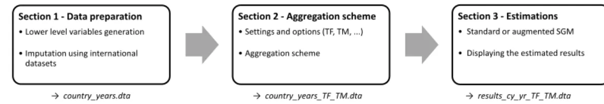
In this part, we present the organization of the Stata programme. The routine is divided in three sections, each section being dedicated to a specic task.
The rst section consists of preparing the data in order to have all needed vari-ables available and ready for the next sections. This includes the verication of data sets integrity (i.e., detecting missing variables and verifying data coherence), the generation of necessary input and output variables, the imputation of missing data, the importation of prices and the construction of indices using both EU-FADN and international data bases1
The second section is dedicated to the settings and options necessary to obtain a given estimation. In particular, the user is invited to choose the type of farm (TF), the time specication (TM) and the aggregation schemes for inputs and out-puts. The routine then generates automatically an adapted data set for further estimations.
Using the previously generated data set, the third and last section is dedicated to estimations using the standard and the augmented Symmetric Generalized Mc-Fadden (SGM) cost function. Figure 2.1 provides a summary of the global Stata routine structure, where the resulting output for each section is shown as a typical .dta le. The next sections give more details about these three specic tasks.
1We resort to international data bases when prices and interest rates are missing in the
EU-FADN dataset. First, we use Eurostat for missing prices and interest rates. If prices and interest rates are still not available in Eurostat, we use OECD, if not the Penn World Table.
Section 1 - Data preparation
• Lower level variables generation • Imputation using international
datasets
Section 2 - Aggregation scheme
• Settings and options (TF, TM, ...) • Aggregation scheme
Section 3 - Estimations
• Standard or augmented SGM • Displaying the estimated results
→ country_years.dta → country_years_TF_TM.dta → results_cy_yr_TF_TM.dta
Figure 2.1: Schematic view of the Stata routine.
2.2 Data Preparation
This rst section of the Stata routine is pre-processing the data in order to have the EU-FADN data sets ready for further manipulations. No specic options or settings are available to the user in this part, except for the choice of the member state or region and the year range to include in the data set.
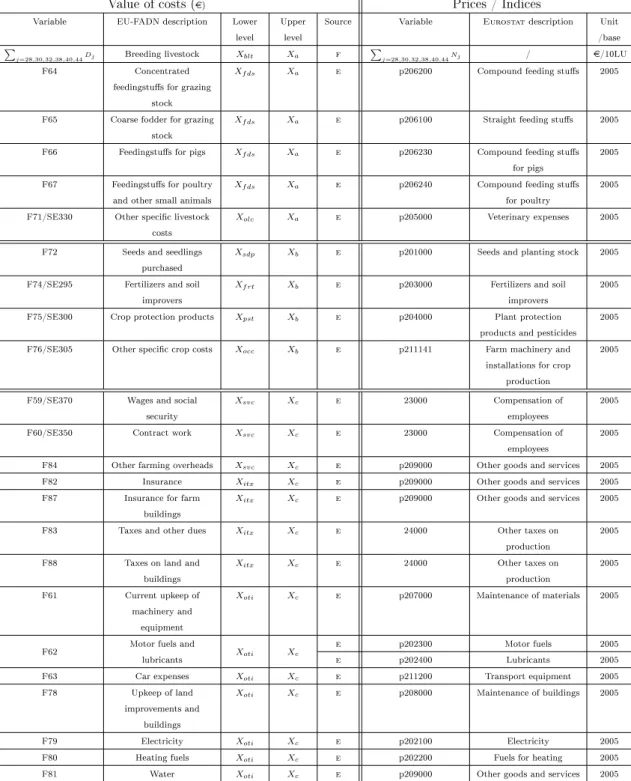
The routine is here divided into two main operations. The rst operation con-sists in constructing every needed variables at the lowest level of aggregation using the EU-FADN data set. Variables are classied into three categories: xed inputs, variable inputs and outputs. It is important to notice that the choice of the aggre-gation at the lowest level of aggreaggre-gation of the variables is an ex ante decision, i.e., once the variable aggregation at the lowest level is decided, the present section of the Stata routine generates the needed aggregated variables at that level, while any other variable at a more disaggregated level is not accessible any more for further estimations. For all these variables, we also construct the farm prices and, when missing, we impute then with the regional prices.2 The second operation consists in importing data from Eurostat, the OECD and the Penn World Table (PWT) in order to impute the remaining missing prices and interest rates. During the two described operations, a special attention is given to the construction of variables adapted to each time specication (medium- and long-term), i.e., input variables that are either xed inputs or variable inputs depending on the time specication.
At the end of this routine, a complete data set including all input and output values and related prices and interest rates is stored in a data le.
2When imputing with the regional prices, the most disaggregated available regional level is
chosen. The scheme for regional levels depends on the availability of regional variables in the EU-FADN dataset.
MIMO Cost Function Estimation for IFM-CAP Model 153916-2013 A08-BE
2.3 Aggregation Scheme
This second section of the routine allows the user to choose between dierent options to make the last data adjustments before estimations. Important options concern the choice of the farm type, the time specication and the resulting aggregation scheme for xed inputs, variable inputs and outputs. The farm type choice allows to select the most relevant farms in the data set, while the choice between the medium- and long-term specications has an inuence on the input aggregation scheme. After choosing the farm type, the user has two possibilities to determine the aggregation scheme. Either, she lets the aggregation scheme to be automatically built by the Stata routine using aggregation schemes that are implemented for each farm type by default, or she chooses the farm type and customizes the aggregation scheme. In that latter case, the user should care to design the scheme in a way that is relevant for the chosen farm type. Once the aggregation scheme is decided either automatically or customized, the routine builds the upper level of variable aggregations following that scheme, i.e., it builds new aggregated variables.
We want to emphasize the fact that exibility resides in the customization of the aggregation scheme. However, as we already mentioned, the only variables that can be used in this aggregation scheme are the ones that have been chosen ex ante and prepared in the rst section of the programme.
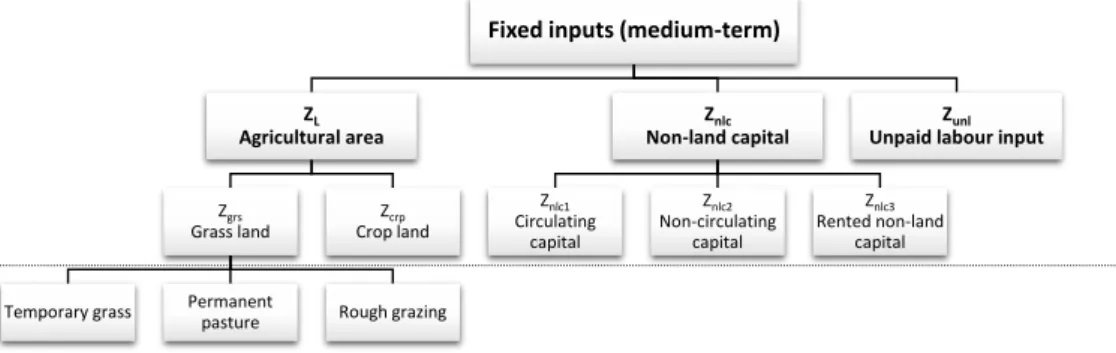
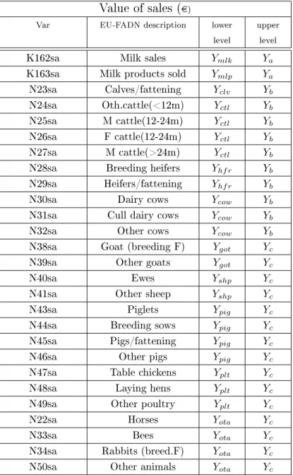
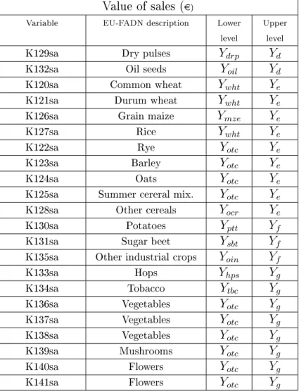
Figures 2.2, 2.3, 2.4 and 2.5 respectively show the aggregation schemes adopted for xed inputs for the medium- and long-term specications, variable inputs for the medium-term specication, variable inputs for the long-term specication and outputs for sale. In each gure, the dotted line marks the limit of disaggregation. Any variable that is below the line is not accessible any more for estimations, while the variables just above the line represent the most disaggregated variables, i.e., those chosen ex ante and constructed in the section for data preparation. The rst line of variables above the dotted line include the variable that are considered at the lower lever of aggregation while the second line of variables above the dotted line include the variables that are consisdered at the upper level of aggregation.
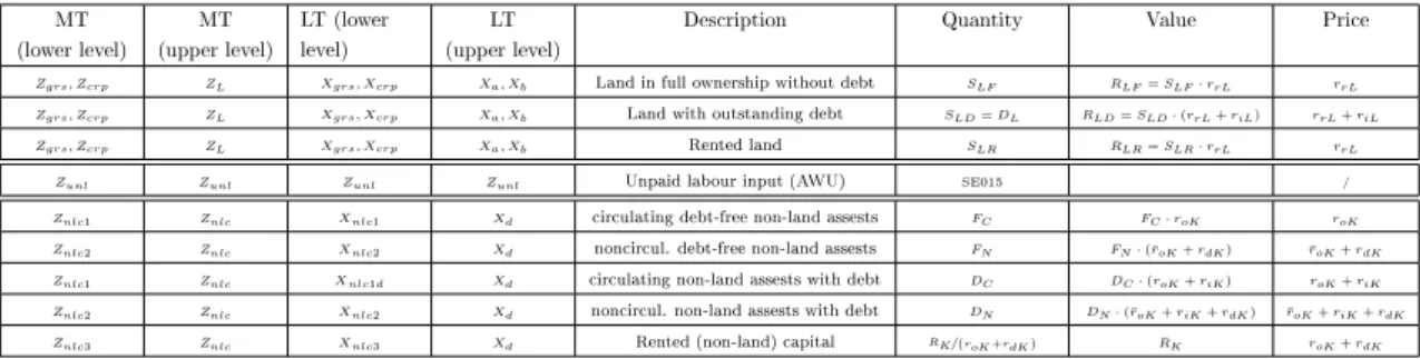
As reported in Figure 2.2 for the medium term, we consider three xed inputs as being agricultural area, non-land capital and unpaid labour input while, for the long term, we only consider one xed input as being unpaid labour input. Accordingly, as reported in Figure 2.4 for the long term, agricultural area and non-land capital become variable inputs (see Chapter 6).
Note carefully that there is no need to single out explicitly on-farm forage crops that are used to feed on-farm animals. Inputs to produce those on-farm forage crops are already counted in the dierent input categories. On-farm forage crops that are
used to feed on-farm animals and, hence, not for sale are intermediate farm inputs. Note in parallel that outputs are only those sold outside the farm. There is no need then to gure out how much inputs are used to grow those on-farm forage crops and how much on-farm crops are produced. Note nally that animal products are denominated in terms of either live animals or dairy products since farms sell those products, nothing else.
At the end of this routine, a data set with only the needed variables for esti-mations is generated, accounting for the chosen type of farm, the time specication and the resulting aggregation scheme.
MIMO Cost Function Estimation for IFM-CAP Model 153916-2013 A08-BE
Fixed inputs (medium-term)
ZL
Agricultural area
Zgrs
Grass land
Temporary grass Permanent
pasture Rough grazing Zcrp Crop land Znlc Non-land capital Znlc1 Circulating capital Znlc2 Non-circulating capital Znlc3 Rented non-land capital Zunl
Unpaid labour input
Fixed inputs (long-term)
Zunl
Unpaid labour input
Figure 2.2: Aggregation scheme for xed inputs (medium- and long-term specica-tions).
V ar ia b le in p u ts (m e d iu m -t e rm ) Xa A ni m al -sp ec if ic inp ut s Xblt B ree di ng lives to ck D ai ry co ws O ther br ee di ng lives to ck Xfds P ur cha sed fee ds G raz ing s to ck C o nc entr at ed fee di ng stuff s C o ar se fo dder fo r gr az ing s to ck Fee di ng stuff fo r pi gs Fee di ng stuff s fo r po ul tr y Xolc O ther s pec if ic lives to ck co sts Xb C ro p -sp ec if ic inp ut s Xfrt Fer ti liz er s Xpst P es ti ci des Xsdp See ds Xocc O ther s p. c ro p co sts Xc O the r i np ut s Xsvc Ser vi ces W age s an d so ci al s ec ur ity C o ntr act wo rk O ther far m ing o ver head s Xitx Ins ur an ce an d ta xes Ins ur an ce Ins ur an ce Ins ur an ce fo r far m bui ldi ng s Tax es Tax es an d o ther dues Tax es o n lan d an d bui ldi ng s Xoti O ther inpu ts m achi ner y Upkeep machi ner y C ar exp ens es Ener gy Moto r fuel s an d lubr ic an ts El ec tr ic ity H eati ng fuel s W at er Upkeep lan d an d bui ldi ng s Figure 2.3: Aggregation sc heme for variable inputs (medium term).
MIMO Cost Function Estimation for IFM-CAP Model 153916-2013 A08-BE V ar ia b le in p u ts (L on g-te rm ) Xa A ni m al -sp ec if ic inp ut s Xgrs G ras s lan d Xblt B ree di ng lives to ck D ai ry co ws O ther br ee di ng lives to ck Xfds P ur cha sed fee ds G raz ing sto ck C o nc entr at ed fee di ng stuff s C o ar se fo dder fo r gr az ing s to ck Fee di ng stuff fo r pi gs Fee di ng stuff s fo r po ul tr y Xolc O ther s pec if ic lives to ck co sts Xb C ro p -sp ec if ic inp ut s Xcrp C ro p Lan d Xfrt Fer ti liz er s Xpst P es ti ci des Xsdp See ds Xocc O ther s p. cr o p co sts Xc O the r i np ut s Xsvc Ser vi ces W age s an d so ci al s ec ur ity C o ntr act wo rk O ther far m ing o ver head s Xitx Ins ur an ce an d ta xes Ins ur an ce Ins ur an ce Ins ur an ce fo r far m bui ldi ng s Tax es Tax es an d o ther dues Tax es o n lan d an d bui ldi ng s Xoti O ther inpu ts m achi ner y Upkeep m achi ner y C ar exp ens es Ener gy Moto r fuel s and lubr ic an ts El ec tr ic ity H eati ng fuel s W at er Upkeep lan d an d bui ldi ng s Xd Non -l an d cap it al Xnlc1 C ir cul at ing Xnlc2 Non -c ir cul at ing Xnlc3 R ented Figure 2.4: Aggregation sc heme for variable input s (long term).
O u tp u ts f or sa le A ni m al o ut pu ts Ya Mi lk o utp uts Ymlk Mi lk Ymlp Mi lk P ro duc ts Yb O ther bo vi ne o utp uts Yclv C al ves fat teni ng Yctl C at tl e M cat tl e (1 2 -2 4 m ) F C at tl e (1 2 -2 4 m ) M cat tl e (>2 4 m ) O ther c at tl (<1 2 m ) Yhfr H ei fer s B ree di ng hei fer s H ei fer s/ fat teni ng Ycow C o ws D ai ry C o ws C ul l da ir y co ws O ther c o ws Yc O ther no n -bo vi ne o utp uts Ygot G o at s G o at (br ee di ng F ) O ther g o at Yshp Sheep Ewes O thersheep Ypig Pigs P ig lets B ree di ng so w P ig s/ fat teni ng O ther pi gs Yplt P o ul tr y Tab le chi ckens Lay ing hens O ther P o ul tr y Yota O ther an im al s H o rs es Bee s R ab bi ts O ther an im al s C ro p o ut pu ts Yd D ry pul ses an d o il see d Ydrp D ry pul ses Yoil O il see d Ye C er eal s Ywh t W heat C o m m o n wheat D ur um wheat Ymze G rai n Mai ze Yrce R ic e Yocr O ther cer eal s R ye B ar ley O at s Sum m er cer eal s O ther cer eal s Yf Indu str ial cr o ps Yptt P o ta to es Ysbt Sug ar beet Yoin O ther indu str ial cr o ps Yg O ther c ro ps Yhps H o ps Ytbc To ba cc o Yotc O ther c ro ps V eg etab les Mus hr o o m s Fl o wer s Figure 2.5: Aggregation sc heme for all outputs.
Part II
Design and Development
of a Method to Prepare and Update
the Data from the EU-FADN
This report on Part 2 focusses on the design and development of the method to prepare and update the data from the EU-FADN for econometric estimations. The data preparation is a two steps process. First, every lower-level variables and their price are generated. This is done for variable inputs, xed inputs and outputs for the medium- and long-term specications. Missing prices are imputed using data from Eurostat. Second, following the choices of the user, including farm type and time specication, the data set is more precisely shaped in order to have only the relevant and needed data left for further estimations. In this second step, variables are aggregated in order to have upper-level variables available too. Two default aggregation schemes are dened, depending on the chosen type of farm: one for bovine farms (livestock and dairy) and one for crop farms. The user may also choose to dene its own aggregation scheme. After data preparation, the resulting dataset contains then both aggregated and disaggregated input and output values (X, respectively Y), input and output prices (W, respectively P) and input and
output quantities (x, respectively y), the level of aggregation being distinguished
using indices.
In general, value and price information for the component items allows the con-struction of a Törnqvist price index for the aggregate. The quotient of aggregate value and Törnqvist index gives the quantity measure value at base-year prices. The construction of these variables is provided in greater detail in this section.
To ensure numerical stability, output quantities and xed input quantities are rescaled such that their mean squared error lies between 1 and 10. For example ym
is transformed into ym(s) = ym·sm sm = 10 −int h log10 √ E[ym]2+Var[ym] i ,
where int[·] denotes the nearest integer.
MIMO Cost Function Estimation for IFM-CAP Model 153916-2013 A08-BE process. This includes the construction of the Törnqvist index, the imputation of prices, the construction of lower-level and the denition of the defaults upper-level aggregation schemes.
Törnqvist Index Construction
Since farm-level aggregate price indices proved too erratic, Törnqvist price indices are constructed at the regional level. They are expressed with respect to base year
t0 = 2005. Törnqvist price indices are generated for every variable at the lower and upper level.1
Supposing all inputsh= 1, . . . ,PI
i=1Ni are grouped intoi= 1, . . . , I categories,
the Törnqvist indexwirt is dened for each input aggregatei, each geographical unit
r and each period t as
wirt = Ni Y j=1 wjrt wjrt0 !gjrt +gjrt 0 2 gjrt = Vjrt PNi k=1Vkrt ,
where Ni denotes the number of input-components encompassed by the aggregate
input i, wjrt represents the average of farm-gate prices of input-component j in
geographical unit r in period t , and Vjrt represents the total value spent on input
j in geographical unit r in period t. We tried dierent geographical subdivisions,
among which individual farms, but nally decided to supply Törnqvist price indices at the regional level, because farm-level aggregate price indices proved too erratic.
Farm-gate prices wjf t for each input-component j at time t for farm f are
ob-tained by dividing the value of total purchases of the farm(Vjf t) by the farm-total
volume purchased(Njf t). An average regional price of inputj in regionr= 1, . . . , R
in periodt is estimated by dividing total purchases within regionr: Vjrt =PFfr=1Vjf t
by total volume purchased Njrt = PFf=1r Njf t. A country-wide price average is
ob-tained similarly. If needed, country-wide average prices are also provided by
Euro-1It is relevant to also generate Törnqvist price indices for lower-level variables since these are
MIMO Cost Function Estimation for IFM-CAP Model 153916-2013 A08-BE stat. Chapter 4 explains how farm-gate input prices are imputed when missing.
Similarly, the Törnqvist index τmrt for output aggregate m in geographical unit
r in period t is given by τmrt = Nm Y n=1 pnrt pnrt0 ! gnrt+gnrt0 2 gnrt = Vnrt PNo o=1Vort ,
where Nm denotes the number of output-components n encompased by the output
aggregate m, pnrt represents the average farm-gate price of output-component n
produced in geographical unit r in period t, and Vnrt represents the total revenue
generated by output-component n in geographical unit r in period t. Average
re-gional and national prices of product n in period t are again obtained by dividing
the value of total production by total number of units sold. Chapter 4 explains how farm-gate output prices are imputed when missing.
Note that average regional or country prices of inputs and outputs are calculated by removing extreme farm-gate prices of inputs and outputs. Farm-gate prices that have a probability of occurence that is smaller than one over twice the sample size are disregarded from that calculation. For input prices, extreme values of wjrt are
dened as
|(wjf t−wjrt)|>Φ−1(1−1/2Fr)∗SDwjf t
whereFr is the sample size,wjrt the regional or country average ofwjf t, and SDwjf t
the standard deviation of wjf t.
Similarly for output prices, extreme values of pnrt are dened as |(pnf t−pnrt)|>Φ−1(1−1/2Fr)∗SDpnf t
whereFr is the sample size, pnrt the regional or country average ofpnf t, andSDpnf t
the standard deviation ofpnf t. Extreme and missing values of farm gate prices are
replaced by their regional or country price average. To preserve the relationship
τmf t =
pmf t
pmf t;b
We use the following denitions for prices of aggregates pmf t = Nm Y n=1 (pnf t) gnft+gnft 0 2 pmf t;b = Nm Y n=1 (pnf t0) gnft+gnft 0 2 .
The price in the base year of an aggregate, pmf t;b, can thus vary from year to year,
Chapter 4
Imputation of Missing Prices
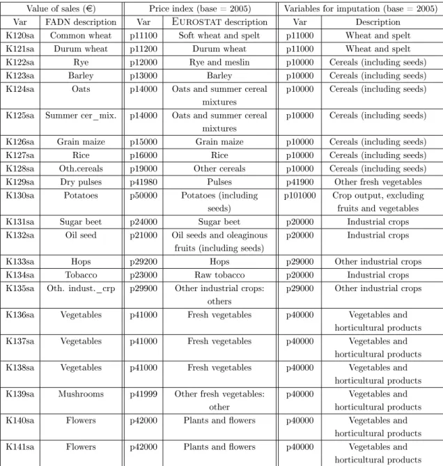
Output prices pnf t are in general computed from sale values and volumes in the
EU-FADN database, if not from production values and volumes. If the necessary information is missing it is supplemented with prices from Eurostat. Information on input prices wjf t is mainly obtained from Eurostat, although for some inputs
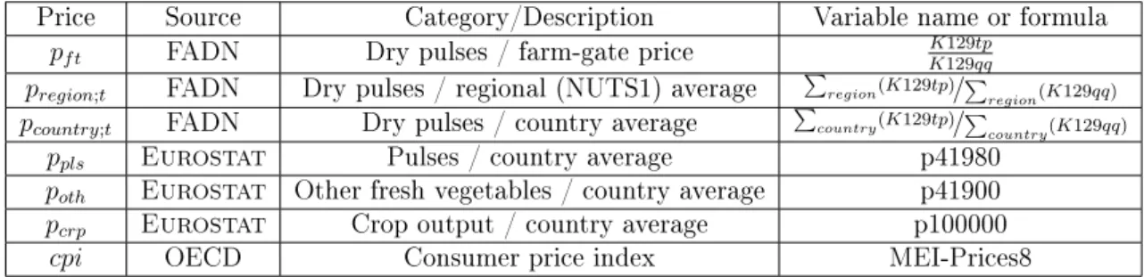
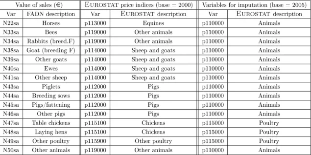
it also stems from the EU-FADN database. Missing prices are imputed according to the following scheme, in which we take dry pulses as an example. From all data sources, we obtain several price variables pertaining to dry pulses (see Table 4.1).
Price Source Category/Description Variable name or formula
pf t FADN Dry pulses / farm-gate price KK129129qqtp
pregion;t FADN Dry pulses / regional (NUTS1) average
P
region(K129tp)/Pregion(K129qq)
pcountry;t FADN Dry pulses / country average
P
country(K129tp)/Pcountry(K129qq)
ppls Eurostat Pulses / country average p41980
poth Eurostat Other fresh vegetables / country average p41900
pcrp Eurostat Crop output / country average p100000
cpi OECD Consumer price index MEI-Prices8
Table 4.1: Illustration of the price imputation scheme using dry pulses as an example We now proceed as follows:
For each observation, i.e., each farm f at each observed periodt, we compute
pf t,pregion;t andpcountry;t. Ifpf t is missing, we assign itpregion;tor, failing that,
pcountry;t.
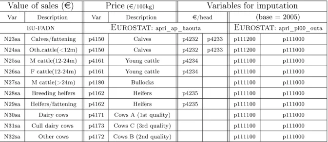
We retrieve price indices from the dataset apri_pi00_outa from Eurostat.1 The Eurostat description of this dataset as well the description of the other datasets that are used in this Part II are shown in Table 4.2. This Table also shows related datasets that are used to impute price variables when they are
1The dataset apri_pi00_outa corresponds to the Price indices of agricultural
missing from the original dataset. From apri_pi00_outa, we take the most detailed index covering the whole crop category (in this example p41980 -pulses), we take the index for the smallest super-category (here Other fresh vegetables) and we take the index covering all crop outputs. Now for each country, and for each pimp=ppls, poth, pcrp, cpi:
if pf t is completely missing, it is replaced by pimp;
if pf t has missing observations, it is regressed on pimp and missing
obser-vations are replaced with the predicted values of this regression.