Economics of air pollution: policy, mortality concentration-response, and increasing marginal benefits of abatement

(1)

Economics of Air Pollution: Policy, Mortality

Concentration-Response, and Increasing Marginal

Benefits of Abatement

A DISSERTATION

SUBMITTED TO THE FACULTY OF THE GRADUATE SCHOOL OF THE UNIVERSITY OF MINNESOTA

BY

Andrew Lloyd Goodkind

IN PARTIAL FULFILLMENT OF THE REQUIREMENTS FOR THE DEGREE OF

Doctor of Philosophy

Jay S. Coggins

(2)

c

Andrew Lloyd Goodkind 2014

(3)

Acknowledgements

I wish offer my greatest appreciation and thanks to those that have shaped my thinking and supported my education. My adviser, Jay Coggins, for inspiring me to study environmental economics and for providing me unwavering encouragement. To the members of my dissertation committee, Julian Marshall, Stephen Polasky and Frances Homans, my education has been greatly enhanced by learning from each of you in classes, as an assistant, and as an adviser to me. My deepest thanks to Chris Tessum, for patiently explaining the details of air dispersion models and selflessly sharing his models and data that were integral to the completion of my dissertation. I want to credit the members of Jay Coggins’ environmental economics special project group, for the fruitful discussions of increasing marginal benefits that helped develop my research topics.

I am forever grateful to my parents, and my wife Amanda for supporting my deci-sions, providing needed encouragement, and making everything I do possible.

(4)

Dedication

To Amanda, my loving wife and best friend.

(5)

Abstract

This dissertation examines the economics of air pollution in three essays. The first two essays consider the implications of the possibility of increasing marginal benefits to pollution abatement. The third essay integrates a new model of air dispersion with an economic model to estimate the marginal damage caused by criteria pollutants in the United States.

In the first essay, the optimal abatement policy is derived for a scenario with increas-ing marginal benefits of abatement and uncertainty in the marginal cost of abatement. Pollution taxes are preferred over quantity restrictions when marginal benefits are in-creasing in abatement.

The second essay uses simulations of fine particulate matter (PM2.5) dispersion and

compares optimal source-specific pollution control policies with pollution concentration standards and uniform pollution taxes. Optimal policies for PM2.5 regulation yield

substantial advantages over uniform policies that do not discriminate based on the location of emissions. The simulations also consider the shape of the concentration-response (C-R) relationship between PM2.5 pollution and mortality. With a log-log

C-R, where marginal benefits of PM2.5 abatement are increasing, society should prefer

fewer emissions and lower PM2.5 concentrations than if the C-R is log-linear, where

marginal benefits of abatement are decreasing.

The third essay estimates the marginal damages of criteria pollutant emissions for hundreds of the most heavily polluting sources in the U.S. Marginal damages vary substantially depending on the location of the emission source. The calculation of marginal damages is highly dependent on the choice of air dispersion modeling, the C-R relationship, and the value assigned to mortality caused by environmental risks.

(6)

List of Tables

3.1 Comparison of abatement policies . . . 67

4.1 InMAP marginal damages . . . 99

4.2 Marginal damages by distance from source . . . 99

4.3 Percent of marginal damages by distance from source . . . 100

(10)

List of Figures

2.1 Increasing marginal benefits: crossing from above/crossing from below . 15

2.2 Tax ranges for four cases . . . 19

2.3 Abatement responses to tax . . . 20

2.4 Tax policy: crossing from above . . . 26

2.5 Optimal tax policy acrossν: crossing from above . . . 27

2.6 Optimal tax policy acrossν: crossing from below . . . 31

2.7 Tax policy: crossing from below, dissimilar slopes . . . 34

2.8 Optimal tax policy acrossν: crossing from above, dissimilar slopes . . . 35

2.9 Optimal tax policy as a function ofν . . . 36

3.1 Relative risk . . . 41

3.2 Marginal cost of abatement . . . 53

3.3 Policy comparison: efficiency vs. uniform standard . . . 60

3.4 Distribution of emissions and PM2.5 concentrations across policies . . . 61

3.5 Optimal standard across C-R . . . 62

3.6 Inequality in PM2.5 concentration across policies . . . 64

3.7 Policy comparison: efficiency vs. uniform tax . . . 66

4.1 Emissions to damages diagram . . . 74

4.2 Source locations . . . 79

4.3 U.S. and source PM2.5 concentrations . . . 81

4.4 2005 and 2013 PM2.5 concentrations . . . 86

4.5 Receptor marginal damages by C-R . . . 89

4.6 VSL by age . . . 94

4.7 Marginal damage: InMAP vs. previous estimates . . . 96

4.8 Distribution of marginal damages across sources . . . 98

(11)

4.10 Ratio of marginal damages of pollutants by distance from source . . . . 102

4.11 Marginal damages by distance and direction from source . . . 104

4.12 Source marginal damages by C-R . . . 105

4.13 Marginal damage function for source . . . 107

4.14 Ratio of marginal damages by VSL method . . . 109

(12)

Chapter 1

Introduction

(13)

This dissertation discusses issues of air pollution and environmental risk. Air pollu-tion that impacts human health is a topic critical to policy makers, businesses and economists. The environmental risks from air pollution, especially fine particulates (particles with diameter less than 2.5 microns, PM2.5), are large and affect almost all

people.

Epidemiologists have identified fine particulate air pollution as a key environmental risk (Popeet al. 1995; Dockeryet al. 1993; Pope, Ezzati and Dockery 2009b). Exposure to all outdoor air pollutants, globally and in the U.S., has been linked with several detrimental health impacts leading to morbidity and mortality including: respiratory infections; lung, trachea and bronchus cancers; ischaemic heart disease; cerebrovascular disease; and chronic obstructive pulmonary disease (Lim et al. 2012). Globally, 3.4 million deaths are attributed to outdoor air pollution annually, 95% of which are from exposure to fine particulates. In the U.S., risks from fine particulate air pollution is the 8th leading cause of mortality, just ahead of alcohol use, responsible for over 100,000 deaths annually, leading to 1.6 million years of life lost (IHME 2014).

With many lives at stake, controlling air pollution is a pressing issue for government regulators and lawmakers. Making comprehensive decisions to limit the external costs of air pollution is difficult for a number of reasons: there are many sources of air pollution, and the connection between emissions and the people impacted is highly complex. With businesses bearing only a fraction of the environmental costs associated with their emissions, air pollution represents an externality that affects an enormous number of people given dispersion of air pollutants and the difficultly avoiding pollution in the air we breathe. Economists play a prominent role in advising policy makers how to appropriately handle the externalities from emissions of pollutants that originate from many sources. Businesses that emit air pollution represent important and central industries in the economy. Given the magnitude of the externalties associated with PM2.5 air pollution, it may be optimal to require businesses to incur large costs to limit

their contributions to pollution, even if it results in dramatic changes to the economy. U.S. government agencies assign large values to health risk reductions of existing and proposed regulations. The Office of Management and Budget estimates benefits of $19 to $167 billion per year from Environmental Protection Agency (EPA) regulations of fine particulates, against costs of $7 billion (OMB 2013). In EPA regulatory impact

(14)

analyses of ozone (EPA 2008), mercury and air toxics (EPA 2011), and carbon (EPA 2014b), the health benefits of reduced mortality risks attributable to fine particulates are included to justify the regulations.

Although these regulations save many lives, an efficient policy of fine particulate air pollution could reap benefits to society between $50 and $220 billion annually, from addi-tional pollution reductions and cost-effective abatement strategies (Muller and Mendel-sohn 2009). Across all outdoor air pollutants with identified monetary damages from increased morbidity and mortality, decreased visibility, and impacts to timber produc-tion, agriculture and recreational activies, the lion’s share of damages are attributable to mortality from chronic exposure to fine particulates. This results from the large mortality risks associated with fine particulate air pollution and the large value placed on avoiding risks to human life.

The impacts of fine particulate air pollution have been identified as an issue of utmost importance by epidemiologists, regulators, and economists, but additional analysis is necessary. This dissertation examines some of the important issues that affect our understanding of the damages from fine particulate air pollution and how they should be regulated.

There exists a disconnect between economic theory of efficient regulation of exter-nalities and most regulations of air pollution. Economics advises pricing emissions of air pollutants at the value of the marginal external damages caused by the emissions. Yet regulators often implement command and control policies requiring emission reduc-tions to meet pollution concentration limits at locareduc-tions of concern, generally without providing financial incentives for polluters to make cost effective pollution abatement decisions. In the U.S., the National Ambient Air Quality Standards (NAAQS) set pol-lution concentration limits that cannot be exceeded in any location.

The reliance on concentration limits for criteria pollutants, in particular PM2.5,

suggests that regulators assume that there are no damages below a particular concen-tration level. In other words, there is a threshhold concenconcen-tration level, below which human health risks are not impacted by further concentration reductions. For expo-sure to PM2.5, results from the two most prominent studies into the link with human

mortality, the American Cancer Society (ACS) study (Pope et al. 2005; Pope et al.

(15)

Laden et al. 2006; Lepeule et al. 2012), indicate that no safe threshhold exists, or that the threshhold is below the concentration levels experienced by most people. If no safe threshhold exists, then there are opportunities to improve public health by fo-cusing attention on reducing risks to people exposed across the entire range of PM2.5

concentrations.

The issue of no safe threshhold of PM2.5 exposure is related to the

concentration-response (C-R) relationship between PM2.5 concentrations and the risk of mortality.

In the most recent analysis of the ACS study, Krewski et al. (2009), estimate two possible functional forms of the C-R: log-linear, a commonly assumed relationship with a constant relative-risk of mortality between any fixed difference in concentration; and log-log, an alternative relationship where the risk of mortality decreases at a faster rate from reductions at low compared to high concentrations. With log-log, the marginal benefits of abating fine particulate pollution are increasing in concentration reductions, suggesting that not only is there no safe threshhold, but the first unit of exposure is the most damaging. The implications of the difference between the log-linear and log-log C-R relationships, for policy and damages from pollution, are explored in the following chapters.

With log-log, a central tenet of environmental economics, that the marginal benefits of abatement are decreasing, is violated. Chapter 2 evaluates the theory of optimal pollution control given increasing marginal benefits of abatement. Here price and quan-tity instruments are compared under marginal abatement cost uncertainty, a framework first developed by Weitzman (1974). The optimal price and quantity policies are de-rived depending on the relative slopes of the marginal benefits of abatement and the marginal abatement costs. The key finding is that, with increasing marginal benefits, a quantity policy is never preferred. Unlike Weitzman (1974), who assumed downward sloping marginal benefits of abatement, the optimal price and quantity policies may yield solutions either at the corners (zero abatement or complete abatement) or in the interior. Another surprising finding is that the optimal price policy is not necessarily at the intersection of the marginal benefit and the expected marginal abatement cost functions. In addition, the optimal price policy is a function of the level of uncertainty in marginal costs. As the level of uncertainty increases, the advantage of the price policy over the quantity policy increases.

(16)

A simulation model is developed in Chapter 3 that analyzes pollution control poli-cies for PM2.5. Dispersion of air pollution from hundreds of sources of PM2.5 emissions

are simulated using a Gaussian plume model, and the resulting pollution concentrations are calculated in receptors for a region of the U.S. Midwest. The model calculates mor-tality risks at each receptor with the log-linear and the log-log C-R from Krewskiet al.

(2009). Three air pollution policies are examined: efficient emission abatement, where the marginal costs of abatement are equated with the marginal benefits of abatement at each source; a uniform pollution limit that cannot be exceeding in any receptor; and a uniform emissions tax.

Important differences are found in the outcomes across the three policies and the two C-R relationships. With a log-log C-R, each policy calls for lower emissions and lower PM2.5 concentrations than with a log-linear C-R. If the true C-R is log-log lower

emissions and concentrations are preferred to take advantage of the larger mortality risk reductions possible in the cleaner locations.

For both C-R relationships, the efficient abatement policy achieves substantially greater welfare for society than the uniform pollution standard. This result highlights the importance of regulating emissions that impact more than just those that face the greatest risks. Finally, substantial advantages exist with the efficient policy com-pared with the uniform emissions tax. While the unform tax achieves a cost-effective outcome, the efficient policy differentiates between the damages of emissions at each location. The spatial heterogeneity of marginal benefits of abatement indicates the im-portance of applying source-specific regulations. One possibile approach to implement an approximation of the efficient abatement policy, with low information requirements of abatement costs by regulators, is a set of discriminating emissions taxes, different for each source equal to the marginal damage of emissions.

In Chapter 4 the marginal damages of emissions of certain criteria pollutants are esti-mated using a newly developed air dispersion model for the U.S. The impact of emissions of PM2.5, SOX, NOX and NH3 (pollutants that contribute to the total fine particulate

concentration), are modeled from hundreds of the largest elevated and ground-level sources of emissions across the U.S. The estimates of the marginal damages of an ad-ditional ton of emissions show orders of magnitude differences depending on source

(17)

location and pollutant. In addition, damages in receptors far from the source of emis-sion can be substantial, highlighting the interconnected nature of the many sources of emissions that contribute to the PM2.5 concentrations in a receptor.

Marginal damages were calculated for each source with the both the Krewskiet al.

(2009) log-linear and log-log C-R relationships. In 2005, the baseline year modeled, fine particulate concentrations were substantially higher than today, and marginal damages with a log-linear and log-log C-R were very similar. However, when the calculations were made with lower 2013 PM2.5 concentrations, the marginal damages with a log-log C-R

were much larger than with a log-linear C-R. At lower fine particulate concentrations, the value of additional emission reductions are larger if the true C-R is log-log.

The results found in Chapters 2, 3 and 4 indicate that using a log-log C-R (or increasing marginal benefits of abatement) can substantially change the analysis of PM2.5 air pollution impacts and regulation. Identifying the true shape of the C-R

between exposure to fine particulates and mortality thus has significant implications for society.

Regardless of the shape of the C-R, fine particulate air pollution is a significant risk to human health that requires attention from epidemiologists and economists. Despite the substantial improvements in air quality in the United States over the last several decades, additional reductions may be required.

(18)

Chapter 2

Prices

vs.

Quantities With

Increasing Marginal Benefits

∗

∗_{Chapter 2 originally as unpublished manuscript with authors:}

Andrew L. Goodkind, Jay S. Coggins, Timothy A. Delbridge, Milda Irhamni, Justin Andrew Johnson, Suhyun Jung, Julian D. Marshall, Bijie Ren, Martha H. Rogers and Joshua S. Apte.

(19)

2.1 Introduction

Environmental policy is often built upon quantity restrictions. In the U.S., at least, these usually take the form of direct quantity standards, with a few noteworthy allowance-trading schemes and emissions taxes mixed in. In this paper we offer new reasons to favor taxes. We find that, for the model under study, quantity restrictions are never preferred and the relative advantage to taxes can be large. In our theoretical model, taxes are preferred because of the flexibility they grant to the polluting industry. The greater the level of uncertainty regarding control costs, the greater the advantage to taxes. Recycling of tax revenue, which we ignore, would tilt the comparison still more decisively in favor of taxes.

In the standard economic model of environmental policy, one assumes that marginal benefits are decreasing or, in the limit, constant in abatement.1 One assumes too that marginal costs are increasing in abatement.2 In this setting, the obvious optimum is found where marginal benefits and marginal costs meet. Familiar textbook treatments of the problem adhere to the standard view. Baumol and Oates (1988, p. 59), to take one prominent example, justify their assumption of downward-sloping marginal benefits this way: “In accord with the usual observations, [MB] has a negative slope, indicating that the greater the degree of purity of air or water that has already been achieved, the less the marginal benefit of a further ‘unit’ of purification.”

This understanding of the curvature of abatement benefits is no longer obviously correct. A benefit function for air pollution abatement is, after all, a reduced form in which is embedded a good deal of nontrivial science. The mapping runs first from abatement to a change in ambient pollution concentration, next from a change in con-centration to a change in health outcomes, and finally from a change in health outcomes to monetary benefits.3 _{If (}_i_{) the first and third mappings are approximately linear; (}_ii₎

1

The limiting case of linear benefits, constant marginal benefits, is employed by Muller and Mendel-sohn (2009).

2

But see Andreoni and Levinson (2001), who argue that the production function for abatement of fine particulates exhibits increasing returns to scale, and thus that marginal costs are decreasing in abatement.

3_{This emphasis on health outcomes reflect that fact that the lion’s share of benefits associated with}

air-quality rules flows from improvements in human health. Of that, the lion’s share flows from avoided mortality. If the curvature of mortality benefits goes against type, it is unlikely that other components such as benefits to avoided hospitalization and morbidity will reverse it.

(20)

the mapping from concentration to health outcomes (a concentration-response function that relates mortality or another negative health outcome to pollution levels) takes the classical logistic form; and (iii) the range of concentration relevant to air policy falls in the convex part of the curve; then one does indeed find support for the “usual ob-servations.” The first unit of abatement is most valuable, the last unit least valuable: marginal benefits are decreasing in abatement.

To be fair to Baumol and Oates, their view reflected the conventional scientific wis-dom of the time. Dockery et al. (1993) and Pope et al. (1995), showed for the first time that there is no safe minimum level of concentration of fine particulates (PM2.5).

Concentration-response (C-R), both papers said, is not logistic but linear. Health dam-age goes all the way down to the lowest observed concentration. Recent evidence sug-gests that linearity itself is now questioned. The C-R, some prominent studies suggest, is strictly concave. Not only is the first unit of concentration not safe, it is the most harmful.

Unexpected benefits curvature can arise from any component of the mapping from abatement to benefits. Nonlinearity due to atmospheric chemistry in the first mapping is a distinct possibility. A curious example, featured in Repetto (1987) and in Muller and Mendelsohn (2012), is that of ozone. Titration of ozone by excess nitrogen oxides means that, in conditions where NOX is plentiful, abatement of NOX can lead to increased

concentration of harmful ozone. Here we have negative and increasing marginal abate-ment benefits for the first units of abateabate-ment, at least for a portion of the downwind landscape.4

If, contrary to the ozone case, the rest of the problem is approximately linear, the curvature of benefits is dual to that of the underlying C-R. Here, if the C-R curve is strictly concave in concentration, then the first unit of concentration is the most harmful, the last unit of abatement the most valuable. In such a case benefits are strictly convex and marginal benefits therefore slope upward in abatement.

This possibility, an unusual observation, forms the intellectual basis for the present

4_{Strange curvature and increasing marginal benefits arise in other situations as well, at least over a}

range of the given policy choice. Examples due to externalities of an intervention include incidence rates for vaccination (Boulier, Datta, and Goldfarb 2007) and for bed nets to prevent malaria (Hawleyet al.

2003). In Anderson, Laxminarayan, and Salant’s (2012) dynamic model of the optimal expenditure of a treatment budget for an infectious disease in multiple villages, unexpected curvature and surprising corner solutions result.

(21)

paper. Why might it be interesting? For PM2.5, according to a growing chorus of

environmental-health experts the curvature of the C-R for this deadly pollutant might be strictly concave.5 Examples include Ostro (2004), Pope et al. (2009a, 2011), and Smith and Peel (2010). These studies rely in part on data representing very high concentrations, for active smokers, that lie outside the range of ambient concentrations observed in U.S. cities.

More compelling evidence, because it relies exclusively upon ambient levels of PM2.5

that are directly relevant to U.S. clean-air policy, is found in Crouse et al. (2012) and Krewski et al. (2009). The Crouse et al. study, in which PM2.5 concentrations range

from 1.9 to 19.2µg/m3, fits natural-spline and logarithmic C-R functions, for four causes of mortality, to a large cohort of Canadian residents. For three of the four categories they cannot reject a linear relationship, but for the fourth (ischemic heart disease) they reject linearity in favor of strict concavity. There, the first unit of concentration is the most harmful, the last unit of abatement the most valuable.6

Krewskiet al.(2009) is especially important because of the role their results play in the U.S. Environmental Agency’s recent (2012b) Regulatory Impact Analysis supporting a new proposed national standard for PM2.5 concentration. Krewskiet al. contains an

extended analysis of the influential American Cancer Society longitudinal study (Popeet al.1995) of the effects of air pollution on human health. In the extended analysis, where PM2.5 concentrations range as low as 5µg/m3, Krewskiet al.estimated a log-linear and

a log-log C-R relating PM2.5 to five causes of death (all causes, cardiopulmonary disease,

ischemic heart disease, lung cancer, and all other causes). Their point estimate of 1.06 for the constant hazard ratio (HR) assocated with all causes of death (see Table 11 of Krewskiet al.2009, p. 28) serves as an essential parameter in the EPA’s (2012b, p. 5-27) PM2.5 benefits assessment.7

5_{Strict concavity is neither unusual nor, apparently, controversial in the case of environmental health}

related to toxins found in workplaces, a threat that lies outside the purview of the U.S. EPA. See, for example, Steenlandet al.(2011) and especially Stayneret al.(2003).

6_{In the Crouse}_{et al.}_{cohort of 2.1 million subjects, ischemic heart disease claimed 43,400 lives between}

1991 and 2001. The corresponding number for all non-accidental causes is 192,300.

7_{In the U.S. EPA PM}

2.5RIA, the 1.06 linear HR estimate from Krewskiet al.(2009) helps determine

the lower end of the range of EPA’s benefits estimate. The corresponding number from Laden et al.

(2006) is 1.16, which helps determine the higher end of the range of EPA’s benefits estimate. Average concentrations in the six cities, all in the eastern U.S., are higher than in the much larger ACS cohort.

(22)

The three right-most columns in Krewskiet al.’s Table 11 report the results of esti-mating a log-log function for each cause of death. These results reflect a strictly concave fitted relationship: the first units of concentration are the most harmful.8 Though they do not report the results of a statistical test to determine which function gives the better fit, Krewskiet al.(2009, p. 27) observe that the log-log form “was a slightly better pre-dictor of the variation in survival.”9 The EPA chose to use the results of the log-linear rather than the log-log model.

Let us state carefully what we endeavor to claim: that a strictly concave C-R, and attendant increasing marginal benefits, might sometimes be true, for some important pollutants and some health endpoints. The scientific results are mixed, and so a stronger claim on our part would be unwarranted. Our point, though, is that this science is unsettled and relatively new. The experts disagree.10 The evidence conflicts.

Our paper is rooted in the following question: What if marginal benefits of abate-ment are increasing. What then is the proper policy response, and which if any of our most familiar recommendations need to be reconsidered?

We examine the effect of increasing marginal benefits on the comparison of tax and quantity instruments in environmental policy (Weitzman 1974). Our focus is not on technology or dynamics or on how different permit-market arrangements affect policy choice.11 Rather, in the presence of increasing marginal benefits we study how corner

8_{It is perhaps worth noting the terminology adopted by Krewski} _{et al.}_{in describing their results.}

The column headings in their Table 11 are given as “Linear” and “Log.” These labels refer to the way in which the PM2.5 variable enters the right side of their regression models. It is either untransformed

(the linear model) or log-transformed (the log model). In both cases, however, the dependent variable is the log of the hazard ratio. (See the unnumbered equations on their p. 27.) Here we adopt the language “log-linear” and “log-log” to refer to the two alternatives. Over the range of ambient PM2.5

concentrations, their log-linear results yield a C-R that is very nearly linear and their log-log results yield a C-R that is markedly concave.

9

Noting the importance of the choice of functional form, they write (2009, p. 28), “The choice of functional relationship between PM exposure and mortality can make a considerable difference in the predicted risk at lower concentrations. For example, the HR for lung cancer adjusted for the ecologic covariates based on the [log-linear] formulation is 1.142 (95% CI, 1.057–1.234), whereas the HR based on the [log-log] formulation is 1.236 (95% CI, 1.114–1.372), a 66% increase in risk.” The corresponding increase for all causes, from 1.078 to 1.128, is 64%.

10_{For an interesting glimpse into the way the scientists talk to each other about curvature, see Schwartz}

(2011).

11_{Karp and Zhang (2012) present a nice overview of the large literature related to the question. They}

study the problem when a regulator behaves strategically. See also Jaffeet al.(2003). Various aspects of the problem of instrument choice are take up by, among others, Moledinaet al.(2003), Fisheret al.

(23)

solutions affect the usual Weitzman-style results.

Given an initial level of air quality, we assume that the marginal benefits of abate-ment and the marginal costs of abateabate-ment are both increasing in abateabate-ment. We allow for the possibility that reducing emissions to zero may be technologically infeasible, per-haps due to background natural sources. In this case, “complete” abatement means a reduction to the minimum feasible level. Expected marginal costs are assumed to meet marginal benefits where abatement is positive but not complete. Then we analyze two sets of cases: those in which marginal benefits are less steep than marginal costs (we call this case “crossing from above”); and those in which marginal benefits are steeper than marginal costs (“crossing from below”).

A model of optimal abatement policy, largely familiar excepting the slope of marginal benefits, is outlined in the following section. There we explain two additional assump-tions, which are adopted throughout: (i) linearity of marginal costs and benefits; and (ii) a uniform distribution on uncertainty. The first is common in the literature since the work of Adar and Griffin (1976). The second is less common, but our wish to characterize the optimal tax requires the selection of a specific functional form for the denisity on the stochastic term. (A normal distribution offers advantages, but it defeats attempts at analytical solutions.) We believe that our results survive in a more general setup, but we defer a detailed analysis of that situation to future work.

Sections 2.3 and 2.4 contain a preliminary analysis of first the optimal quantity policy and then the optimal price policy. If marginal benefits are steeper than marginal costs, we show that the optimal quantity policy is either zero or maximum possible abatement. The optimal price policy is more complicated because for a given tax it is possible that for some realizations of the stochastic term the industry will choose either zero abatement or maximum possible abatement. The corners that come into play add a significant degree of complexity to the tax-setting regulator’s optimization problem.

Section 2.5 addresses the problem for the situation of marginal benefits crossing from above. In this case the optimal price is always preferred. This finding is not at odds with Weitzman, but we find that if the level of uncertainty becomes sufficiently large, the optimal emissions tax is no longer at the intersection of marginal benefits and

explored by Montero 2002, Milliman and Prince (1989), Biglaiser et al.(1995), Gersbach and Glazer (1999), and Requate and Unold (2003).

(24)

expected marginal costs.

Section 2.6 contains the heart of the paper. There marginal benefits cross marginal costs from below. The all-or-nothing nature of the quantity policy means that the welfare stakes are especially high, in that the regulator might choose a policy of zero abatement when the optimal policy was maximum possible abatement. If the level of uncertainty is low, the price and quantity policies are equivalent. If the level of uncertainty is sufficiently high, the price policy becomes strictly preferred. At the threshold, the optimal tax can jump discretely from extreme (either high or low) to an intermediate level.

The intuition for this result goes as follows. If the regulator had perfect informa-tion about costs, the appropriate policy, either zero abatement or maximum possible abatement, could be selected with confidence. This is essentially the outcome achieved by either policy if uncertainty is low. If the level of uncertainty is high, though, the quantity policy is likely to produce the incorrect level of abatement. The wrong choice, in either direction, can be quite costly. An intermediate tax, however, allows the regu-lator to exploit the fact that the industry will choose low abatement (if the realization of uncertainty is high) precisely when zero abatement was optimal and will choose high abatement (if the realization of uncertainty is low) precisely when maximum possible abatement was optimal. The tax policy confers an advantage via the flexibility granted to the industry, whose interests are, in a crucial sense, aligned with those of the regula-tor.

2.2 The basic model

Consider the problem facing a regulator who contemplates limiting emissions of a single pollutant from a single polluting industry. Current total emissions are eT > 0. Due to technological constraints the minimum achievable level of emissions is emin > 0. The corresponding maximum level of abatement is denoted e0 < eT and abatement is a ∈[0, e0_{]. (Abatement levels greater than} _e0 _{are ignored throughout, and abatement}

ate0 is referred to as complete abatement.) The nonstochastic benefit to abatement is described by the quadratic function B : [0, eT] → _R₊ given by B(a) = αa+ (β/2)a2,

(25)

with α≥0,β >0, andB(0) = 0. Marginal benefits are written

MB(a) =α+βa

and are known by the regulator with certainty.

The industry’s cost of abatement is quadratic on [0, e0], but because further abate-ment is infeasible (and so infinitely costly) we ignorea > e0and writeC : [0, e0]×R→R. The cost function depends upon abatement and upon a random variable u, and is ad-ditively separable in its two arguments: C(a, u) =ηa+ (δ/2)a2+ua, withη≥0, δ >0 and C(0, u) = 0 for any u. Marginal costs are written

MC(a, u) =η+δa+u.

Let the vector of structural parameters be denoted θ= (α, β, η, δ, e0).

Uncertainty enters only through the distribution on the intercept of marginal costs. Let the support for the intercept be on the finite interval [η−ν, η+ν], with ν > 0. The density function for u within this interval is assumed to be uniform, with density f(u) = 1/2ν and with E(u) = 0. We assume that the regulator knows the density functionf(u). Social welfare is quadratic in abatement, and is given by

SW(a, u) =B(a)−C(a, u)

We shall assume throughout that marginal benefits and expected marginal costs intersect exactly once, in the interior of [0, e0_{]. We then distinguish between situations}

in which marginal benefits cross marginal costs from above and from below. These are formalized as follows.

Assumption 1. (Crossing-from-above condition.) There exists â ∈ (0, e0) such that MB(a) > E MC(a, u) for all a ∈ [0,â) and MB(a) < E MC(a, u) for all a ∈ (â, e0].

Assumption 2. (Crossing-from-below condition.) There exists ˆa ∈ (0, e0) such that MB(a) < E MC(a, u)

for all a ∈ [0,ˆa) and MB(a) > E MC(a, u)

for all a ∈ (ˆa, e0].

(26)

ˆ a ˆ t e0 eT MB(a₎ E_[MC]

A

abatement (a₎ $/ a ˆ a ˆ t e0 eT MB(a₎ E_[MC] X Z

B

abatement (a₎ $/ a

Figure 2.1: Depiction of upward-sloping marginal benefits. A: crossing from above. B: Crossing from below.

Assumption 1, which implies thatα > ηandβ < δ, is depicted in Figure 2.1A, where MC(a,0) represents marginal cost with degenerate u. A quantity-setting regulator in this situation would maximize expected social welfare by setting abatement at ˆa. A price-setting regulator would maximize expected social welfare by setting an emissions tax at or near ˆt.

Assumption 2, which implies that α < η and β > δ, is depicted in Figure 2.1B. There, the optimal abatement level depends upon whether area X is less than or greater than area Z. In either case, abatement at ˆa, the crossing point, results in negative social welfare, the minimum to the regulator’s optimization problem. This will be true of the intersection any time the curves satisfy Assumption 2. We will see that under Assumption 2, with uncertainty the optimal emissions tax is ill-behaved in the face of uncertain costs.

2.3 The optimal quantity policy

Suppose that the random term in MC(a, u) is degenerate atu= 0. Under Assumption 1, the problem without uncertainty is straightforward. The optimal quantity policy is set

(27)

where MB(a) = MC(a,0). Under Assumption 2, the optimal quantity policy is either maximum possible abatement or no abatement. In either case, there exists a critical value η∗ such that the social welfare associated with maximum possible abatement is zero. This value is given by

η∗= e

0

2(β−δ) +α. (2.1)

The optimal quanity policy is defined by the relative value of the intercept of the ex-pected marginal cost curve and η∗

q∗(η) =          e0 _if_{η < η}∗ {0, e0} ifη=η∗ 0 ifη > η∗. (2.2)

With uncertainty in marginal cost, whether she chooses to pursue a price policy or a quantity policy, our regulator is assumed to maximize expected social welfare. The optimal quantity policy is based entirely upon the intersection of marginal benefits and

expected marginal costs. The quantity-setting regulator’s optimal decision ruleq∗(ν;θ) maximizes expected social welfare:

q∗(ν;θ) = argmax q∈[0,e0_] Eu Z q 0 MB(a)−MC(a, u)da . (2.3)

This constraint set for q is compact inRand the objective function is continuous in q. By the Weierstrass Theorem it achieves a maximum. If marginal benefits cross from above (Assumption 1 holds), the optimal quantity policy is at ˆa, where the two curves meet. If marginal benefits cross from below (Assumption 2 holds), the optimal quantity policy is once again given by equation (2.2) and is either zero or e0.

2.4 The optimal price policy

If there is no uncertainty, the price policy, an emissions tax of t, mimics the quantity policy. If marginal benefits cross from above, it is set where MB = E[MC(a, u)]. If marginal benefits cross from below, it is set either where t ≥ MC(e0) (if η < η∗) or where t ≤ MC(0) (if η > η∗). Because any tax at or less than MC(0) is equivalent,

(28)

and any tax at or greater than MC(e0) is equivalent, we limit attention to those inner thresholds.12 For the knife-edge case with η =η∗, the regulator is indifferent between the upper and lower taxes. The optimal tax policy with no uncertainty is

t∗(η) =          MC(e0) ifη < η∗ MC(0),MC(e0) ifη=η∗ MC(0) ifη > η∗. (2.4)

If there is uncertainty in costs, the price policy depends upon more than expected marginal cost, for the industry’s chosen level of abatement depends upon the realization of u. The abatement response creates a price corner that is quite different from the all-or-nothing quantity corner that arises, even without uncertainty, when Assumption 2 is satisfied.

Clearly, if t ≤ MC(0,−ν) the outcome will be zero abatement. Define tmin =

MC(0,−ν) and note that any t ≤ tmin serves as a zero-abatement policy. We ignore

t < tmin as redundant. Ift≥MC(e0, ν) the outcome will be maximum possible

abate-ment. Define tmax = MC(e0, ν) and note that any t≥tmax serves as a full-abatement

policy. We ignore t > tmax as redundant. The interesting cases lie between these

two extremes. There, the industry will attempt to respond to t by choosing ˜a so that t = MC(˜a, u). Given that marginal cost, being continuous and strictly monotone in-creasing, is invertible, on the interval u ∈

t−E MC(e0, u) , t−E MC(0, u) the function describing the abatement level at which realized marginal cost equalstis given by

˜

a(t, u) = t−η−u

δ . (2.5)

12_{Here we hew to the literature in assuming implicitly that there is no deadweight loss associated with}

taxation. The tax revenue oft∗e0 in the zero-abatement situation is simply a transfer from polluters to the regulator. Under Assumption 2, the question of deadweight taxation losses can be mooted by imposing a tax of zero whenever η > η∗. At the other extreme, of course, if abatement is ate0 there are no emissions and so no tax is paid at all.

(29)

For the industry, the optimal abatement level given tis therefore a∗(t, u) =          e0 ifu≤t−E MC(e0, u) ˜ a(t, u) ift−EMC(e0, u)< u < t−EMC(0, u) 0 ifu≥t−EMC(0, u). (2.6)

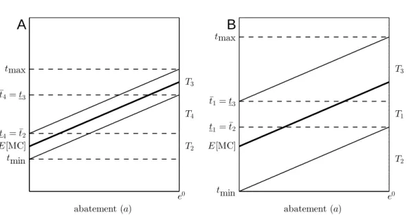
The interval of interesting taxes may be partitioned usefully, as illustrated in Fig-ure 2.2. Consider first FigFig-ure 2.2A, where uncertainty is relatively low. For taxes below tmax but above MC(e0,−ν) (this threshold is denoted t4 =t3 in the figure), the

indus-try’s abatement response will be eithere0 with positive probability (for low realizations of u) or interior (for high realizations). Denote by T3 the interval of tax levels at which

this corner can arise. One price corner, where abatement turns from the maximum pos-sible to interior, resides in T3. For taxes above tmin but below MC(0, ν) (this threshold

is denoted t₄=t2 in the figure), with positive probability the industry’s abatement

re-sponse will be zero (for high realizations ofu) or it will be interior (for low realizations). Denote by T2 the interval of tax levels at which this corner can arise. Another price

corner, where abatement turns from zero to interior, resides in T2. Between T2 and T3

is a band of tax levels at which abatement is sure to be interior. Denote this interval T4.

Now consider a situation in which uncertainty has risen. In Figure 2.2B, this is depicted as an increase in ν. If, as here, the increase is large enough that MC(0, ν) ≥ MC(e0,−ν), then the inner endpoints of T2 and T3 switch places, though tax levels in

the two intervals encounter the same corners as before. When it is nonempty, as in Fig-ure 2.2B, the region betweenT2andT3, now denotedT1, is fundamentally different from

theT4 region in Figure 2.2A. At anyt∈T1, according to the response function in (2.6)

there is positive probability of a= 0 (for high realizations of u), of interior abatement a ∈ (0, e0) (for intermediate realizations of u), and of a = e0 (for low realizations of u). In fact, whenever T1 6= ∅ there is no tax at which abatement is guaranteed to be

interior.13

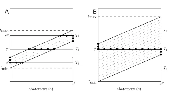
The price corners are usefully depicted in Figure 2.3, which shows the industry’s

13

Avoiding the price corner, Weitzman (1974) considers only tax levels inT4, where abatement is sure

(30)

t_min t₄₌t¯₂ ¯ t₄₌t 3 t_max E_[MC] e0 T₂ T₄ T₃

A

abatement (a₎ t_min t 1=¯t2 ¯ t₁₌t₃ t_max E_[MC] e0 T₂ T₁ T₃

B

abatement (a₎

Figure 2.2: Tax ranges for four cases. A: uncertainty is low,T4 is nonempty. B: uncertainty is high, T1 is nonempty.

response to different tax levels. (The dashed lines represent possible realizations of marginal costs.) In Figure 2.3A, which corresponds to Figure 2.2A, three different taxes are illustrated. At t0 ∈ T2, abatement will be zero for high and interior for low

realizations ofu. Att000∈T3, abatement will be ate0 or interior. Att00∈T4, abatement

must be interior. In Figure 2.3B, which corresponds to Figure 2.2B, we see that at t00∈T1 all three responses are possible: zero, interior, or maximum possible abatement

for high, intermediate, or low realizations of u.

More formally, take a permissible parameter vector (θ, ν), and defineT = [tmin, tmax].

Partition T as described above, where the suprema and infima of theTj are given by

t₁ = MC(e0,−ν) t1 = MC(0, ν) (2.7a) t₂ =tmin t2 = min MC(e0,−ν),MC(0, ν) (2.7b) t₃ = maxMC(e0,−ν),MC(0, ν) t3 =tmax (2.7c) t₄ = MC(0, ν) t4 = MC(e0,−ν). (2.7d)

(31)

t min t_max t′ t′′ t′′′ e0 T₂ T₄ T₃

A

abatement (a₎ t min t_max t′′ e0 T₂ T₁ T 3

B

abatement (a₎

Figure 2.3: Abatement responses. A: T4 is nonempty. Abatement is zero or interior at t0; interior at t00; complete or interior att000. B: T1 is nonempty. Abatement is zero, interior or complete at t00.

The elements of the partition are

T1=    [t₁, t1] ift1 ≤t1 ∅ otherwise T2 =    [t₂, t2] ifT1=∅ [t₂, t2) ifT16=∅ T3=    [t₃, t3] ifT1=∅ (t₃, t3] ifT16=∅ T4 =    (t₄, t4) ift4< t4 ∅ otherwise. (2.8)

Because of the way they are defined, T1 = ∅ precisely when T4 6= ∅. This is true

if MC(0, ν) < MC(e0,−ν). Conversely, T4 = ∅ precisely when T1 6=∅. This is true if

MC(0, ν) ≥ MC(e0,−ν). To see that equations (2.8) constitute a partition, note that Tj∩Tj0 =∅for all j 6=j0 and also that ∪_jT_j =T. The two-part definitions for T₂ and T3 ensure that the partitions do not intersect, as uncertainty increases, at the point at

which T1 appears as a singleton set with t= MC(0, ν) = MC(e0,−ν).

(32)

according to whether abatement is at e0, interior, or zero: SW(t, u) =          B(e0)−C(e0, u) ifu≤t−E MC(e0, u) B ˜a(t, u)−C ˜a(t, u), u ift−EMC(e0, u)< u < t−EMC(0, u) B(0)−C(0, u) ifu≥t−EMC(0, u). (2.9) The tax-setting regulator’s optimization problem may be obtained as follows. Inte-grate (2.9) over the support of u, separating the three subintervals in [−ν, ν]. One or two of these intervals may be empty for some values of t. The first integral in (2.10) is over all realizations of u that yield maximum possible abatement and the second is over realizations for which abatement is interior. The third integral, over realizations for which abatement is zero, yields zero expected welfare and so can be discarded. The optimal tax, which maximizes expected social welfare, is the solution correspondence

t∗(ν;θ) = argmax t∈[tmin,tmax] Z max −ν,minν,t−E[MC(e0_,u₎_] −ν B(e0)−C(e0, u) f(u)du + Z min ν,max−ν,t−E[MC(0,u)] max−ν,minν,t−E[MC(e0_,u_)] B ˜a(t, u) −C ˜a(t, u), u f(u)du + Z ν minν,max−ν,t−E[MC(0,u)] [0]f(u)du (2.10)

where f(u) = 1/2ν. The min{·,·} and max{·,·} operators in the limits of integration ensure that each integral is evaluated over the correct interval. The outer max{·,·} function on the upper limit of the first integral, for example, determines whether the infimum of T3 is given by MC(e0,−ν) (when T4 6=∅) or by MC(0, ν) (when T1 6= ∅).

The inner min{·,·} function then determines whether the limit is determined by the upper boundaryν ofuor by the value of uat which abatement moves into the interior. This is a price corner.

The constraint set for tin (2.10) is compact in Rand the objective function is con-tinuous in t. By the Weierstrass Theorem it achieves a maximum. But the task of selecting the optimal tax is not trivial. This is because of the non-differentiable func-tions, containing the choice variablet, that define the limits of integration. Were those functions differentiable, first-order necessary conditions for (2.10) could be obtained via

(33)

Leibniz’s rule. Because they are not, the only available strategy for deriving the opti-mal tax is to define separate functions for expected social welfare on the Tj. Fort∈T1

there are possible tax levels in all three of the components of integral (2.10). For t∈T2

there is no realization of u at which abatement will be e0. There, only the second and third integrals in (2.10) are relevant. For t ∈ T3 there is no realization of u at which

abatement will equal zero. The first two components of (2.10) are relevant. For t∈T4

it must be true that a∈(0, e0), so only the second component of (2.10) is relevant. Define the following four functions describing expected social welfare on the corre-sponding Tj: Γ1:T1 →R, with Γ1(t) = Z t−E[MC(e0,u)] −ν B(e0)−C(e0, u)f(u)du + Z t−E[MC(0,u)] t−E[MC(e0_,u_)] B ã(t, u) −C ã(t, u), u f(u)du (2.11) Γ2:T2 →R, with Γ2(t) = Z t−E[MC(0,u)] −ν B ã(t, u)−C ã(t, u), uf(u)du (2.12) Γ3:T3 →R, with Γ3(t) = Z t−E[MC(e0,u)] −ν B(e0)−C(e0, u) f(u)du + Z ν t−E[MC(e0_,u_)] B ã(t, u)−C a˜(t, u), uf(u)du (2.13) Γ4:T4 →R, with Γ4(t) = Z ν −ν B a˜(t, u) −C ã(t, u), u f(u)du. (2.14)

The functions Γ1 and Γ4 in (2.11) and (2.14) are quadratic in t; Γ2 and Γ3 in (2.12)

and (2.13) are cubic in t. All four are therefore continuously differentiable int. Piecing them together yields the function describing expected social welfare on all of T. This function is also continuously differentiable, though there may be multiple local maxima and minima: E[SW(t, u)] =                  Γ1(t) ift∈T1 Γ2(t) ift∈T2 Γ3(t) ift∈T3 Γ4(t) ift∈T4.

(34)

which T1 =∅. In either case, the relationships between equations (2.11)–(2.14) at the

boundaries of the Tj ensure that the price-setting regulator’s problem is well behaved: the E[SW(t, u)] function is twice differentiable.

Our goal is to identify the values of t at which expected social welfare might be maximized. This requires finding all values at which the derivatives of (2.11)–(2.14) are equal to zero. Differentiating all four expressions with respect to t, setting the results equal to zero, and solving for t in each case produces six candidate zeros and leads to the following collection of candidate optima:

ˆ t1 =α+ βe0 2 (2.15) ˆ t2a=η−ν and ˆt2b = β(η−ν)−2αδ β−2δ (2.16) ˆ t3a=η+δe0+ν and ˆt3b = β(η+ν)−βδe0−2αδ β−2δ (2.17) ˆ t4 = βη−αδ β−δ . (2.18)

Note that neither ˆt1 nor ˆt4 depends upon ν, and ˆt4 is the tax that equates marginal

benefits and expected marginal costs. In all cases, we have tmin ≡ ˆt2a and tmax ≡

ˆ

t3a. Depending on the parameter vector, some of the conditions in (2.15)–(2.18) might

describe either a local maximum or a local minimum. Separating them, essential in order to identify the optimal policy overall, involves analyzing a set of second-order sufficient conditions. That analysis, lengthy and somewhat tedious, is available in Appendix B.

2.5 Prices

vs.

quantities: Crossing from above (

β < δ

)

Suppose that Assumption 1 is satisfied, so that marginal benefits cross marginal costs from above. That is,β < δ. In this case the following threshold values ofν are relevant. [See Appendix B.] They are important in determining (2.23), the function describing

(35)

the optimal tax: ν1A=E[MC(e0, u)]−MB(e0)− e0β 2 (2.19) ν1B= MB(0)−E[MC(0, u)] + e0β 2 (2.20) ν4A= δ[E[MC(0, u)]−MB(0)] β−δ (2.21) ν4B= δ[MB(e0)−E[MC(e0, u)]] β−δ . (2.22)

Asν increases beyond the relevant thresholds, progressively more probability is pushed away from the neighborhood of the intersection of MB(a) andE[MC(a, u)] and, eventu-ally, piles up ata= 0 and ata=e0. There, the price policy is unambiguously preferred to the quantity policy, which is locked immovably at q∗ = ˆa. More probability at the corners means that the advantage to the price policy is greater.

The optimal tax rule under Assumption 1 is given by

t∗_[_β<δ_](ν;θ) =                  ˆ t1 if [η≥η∗ and ν ≥ν1A] or [η≤η∗ and ν≥ν1B] ˆ t2b if [η > η∗ and ν ∈[ν4A, ν1A) ] ˆ t3b if [η < η∗ and ν ∈[ν4B, ν1B) ] ˆ t4 if [η≥η∗ and ν < ν4A] or [η≤η∗ and ν < ν4B]. (2.23)

Recall that at the threshold η∗, found in equation (2.1), expected social welfare at maximum possible abatement is zero. If η < η∗, expected social welfare at maximum possible abatement is positive; if η > η∗ it is negative. The elements that make up equation (2.23) may be divided along these lines.

The optimal price is ˆt4 when the level of uncertaintyν is sufficiently small, with the

threshold depending upon whetherη is greater than or less thanη∗. This price is at the intersection of marginal benefits and expected marginal costs. When ν is sufficiently large the optimal price, ˆt1, diverges away from this intersection, with the threshold

again depending upon whether η is greater than or less than η∗. The optimal price is intermediate, either ˆt2b or ˆt3b, when ν is also intermediate.

(36)

policy strictly dominates a quantity policy, and the advantage grows with ν, when Assumption 1 holds. (Proofs of this and the remaining propositions appear in Appendix A.) Under the optimal price policy, the level of emissions selected by the polluting industry moves toward the optimum. Under the optimal quantity policy this adjustment is impossible. Expected social welfare under the quantity policy is unchanged as ν increases, but expected social welfare under the price policy grows as ν increases.

Proposition 1. For any permissible parameter vector(θ, ν)at whichβ < δ, the expected social welfare resulting from the optimal price policy is not less than that associated with the optimal quantity policy: E[SW(t∗(ν;θ), u)] ≥ E[SW(q∗(ν;θ), u)]. If ν > 0,

E[SW(t∗(ν;θ), u)]−E[SW(q∗(ν;θ), u)] is strictly positive and strictly increasing inν.

A central tenet of the literature comparing price and quantity policies is that the price policy should be set at ˜t, where marginal benefits equal expected marginal costs. As the level of uncertainty increases, for the linear-uniform case examined here this is not always true. This is due to the fact that, for high levels of uncertainty, a price at the intersection cannot capture the welfare gains associated with realizations far from expected marginal costs. The following result establishes conditions under which the received wisdom is overturned.

Proposition 2. Consider a permissible parameter vector (θ, ν) at which β < δ.

(i.) Suppose η > η∗. If ν > ν4A then t∗ >t˜.

(ii.) Suppose η < η∗. If ν > ν4B thent∗ <˜t.

Example 1. A numerical example might help to illuminate these results and the com-plex nature of the regulator’s optimal tax-setting rule. For the linear-uniform situation under consideration, suppose that the parameter values are

α= 80, β = 1, η= 60, δ = 2, e0= 50.

Figure 2.4 shows the four Γj(t) curves that combine to form the regulator’s ob-jective function E[SW(t, u)], which is the bold curve. It is constant outside of the interval [tmin, tmax]. This figure illuminates several important features of the

(37)

20 40 60 80 100 120 140 160 180 200 −300 −200 −100 0 100 200 300 E[SW(t,u)] E[SW(t⋆_{, u}_)] t⋆ _t_¯ 4 t₄ t_min tmax Γ2(t) Γ3(t) Γ4(t) Γ1(t) tax (t) E [S W ( t, u )] ($)

Figure 2.4: Outcome from all possible taxes, and the four Γj functions with ν = 20, T1 = ∅,

α= 80,β= 1, η= 60> η?, and δ= 2.

indeed quadratic functions. Another is that the three feasible SW curves join as claimed, and are also differentiable where they join at t₄ = 80 and t4 = 140. Thus, the global

E[SW(t, u)] function is differentiable. Note that, with T1 = ∅, Γ1(t) is not a part of

the E[SW(t, u)] function. In this example, ν = 20< ν4A, the optimal price is ˆt4 at the

intersection of marginal benefits and marginal costs. For higher values ofν,T4 becomes

empty and theT1 interval comes into play.

Figure 2.5 shows how things change asν, the level of uncertainty, increases. There, the five curves represent expected social welfare, as a function of the tax, forν ranging from 10 to 60. For any ν > 0, the optimal price policy yields higher expected social welfare than does the optimal quantity policy. As uncertainty grows withν, the expected social welfare associated with the optimal tax also grows and, atν= 60, is almost thrice

(38)

20 40 60 80 100 120 140 160 180 200 −300 −200 −100 0 100 200 300 400 500 600 700 E[SW(q⋆_{, u}_)] t⋆₍ ν) ν= 10 ν= 30 ν= 40 ν= 50 ν= 60 tax (t) E [S W ( t, u )] ($)

Figure 2.5: E[SW(t, u)] and t? as uncertainty increases withα= 80,β = 1, η = 60> η?, and

δ= 2.

that at ν = 10. Higher uncertainty, it turns out, is better.14 Meanwhile, the expected social welfare of the optimal quantity policy remains at 200.

The vertical and piecewise-linear object labelled t∗(ν) in Figure 2.5 shows how the optimal tax changes continuously as ν grows. For ν ≤40 we find that t∗ = ˆt4 = 100,

the price at which MB(a) andE[MC(a, u)] intersect. Forν ≥55,t∗ = ˆt1 is constant at

105. Between ν = 40 and ν = 55, the optimal tax, ˆt2b, rises linearly in ν.15 (See also

14

Greater uncertainty can be an advantage in Weitzman (1974, p. 485) too: “Theceteris paribus effect of increasingσ2 is to magnify the expected loss from employing the planning instrument with compar-ative disadvantage.” In his model the expected social welfare under a quantity policy is unchanged in the face of increasingσ2. Therefore, expected social welfare under a price policy must increase withσ2. One might reasonably observe that increased uncertainty is unlikely to make society better off. The fact that it does so here, as in Weitzman, is a result of the assumptions that the polluting industry knows its cost function with certainty and the regulator knows the distribution of uncertainty exactly. If the industry were itself uncertain about its costs, as is more likely to be the case in practice, the effect of greater uncertainty may be quite different.

15_{In this example we have} _{η > η}∗

(39)

Figure 2.9, where the relationship between t∗ and ν is even more clear.)

2.6 Prices

vs.

quantities: Crossing from below

The situation examined in the previous section is not different in essence from the Weitzman framework with marginal benefits sloping downward but less steeply sloped than marginal costs. Even though our marginal benefits slope upward, Weitzman’s basic insight is preserved: when marginal benefits are more nearly horizontal than marginal costs, a price policy is strictly preferred.

In this section, which concerns cases in which Assumption 2 is satisfied (that is, α < η and β > δ), we enter unexplored terrain. Because the optimal quantity policy is now discrete, all or nothing, the comparison to a price policy becomes both more complicated and more important. Complicated because a new kind of corner solution and a new discontinuity appear, and important because the stakes involved in choosing the right policy become greater. Choosing maximum possible abatement when zero abatement is optimal, or vice versa, can lead to very large welfare losses. And choosing anything in the middle, which can occur when an intermediate tax is selected, risks the greatest losses of all. We will see that this risk is sometimes worth taking.

It turns out that another surprise awaits us. The problem, and especially the be-havior of the optimal tax policy, depend crucially on the difference between the slope of marginal costs and the slope of marginal benefits. Our results are for the linear-uniform case to which we have restricted attention, but it appears that a similar result will go through for a more general setup. Here, the behavior depends upon whether β is less than or greater than twice δ. Much of the section is divided along these lines. The reader should bear in mind that, in the entire section, equations (2.6) through (2.18) are still in force.

Before turning to an examination of the two cases, we pause to establish an initial result that applies whenever marginal benefits cross from below, whether β < 2δ or β ≥2δ. Proposition 3 shows that a quantity policy can never outperform the optimal price policy when marginal benefits cross from below.16

that the optimal tax movesbelow the intersection of MB andE[MC].

16

Note that we have not restricted realized marginal costs to remain positive, which they do not wheneverη < ν. In that case any negative tax, including importantlytmin=η−ν <0, can be thought

(40)

Proposition 3. For any permissible parameter vector(θ, ν)at whichβ > δ, the expected social welfare resulting from the optimal price policy is not less than that associated with the optimal quantity policy: E[SW(t∗(ν;θ), u)]≥E[SW(q∗(ν;θ), u)].

2.6.1 Similar slopes: δ < β <2δ

We turn first to the case in which marginal benefits cross from below, but the slope is less than twice that of marginal costs: β ∈(δ,2δ). Throughout, whenever Assumption 2 is satisfied and soβ > δ, from equation (2.18) we know that ˆt4is a local minimum when

T4 is feasible. We can ignore ˆt4 in our search for the optimal tax.

The optimal tax rule, analogous to equation (2.23) is given by

t∗_[_β_∈(_δ,₂_δ_)](ν;θ) =                        tmin if η≥η∗ and ν ≤E[MC(0, u)]−MB(0) ˆ t2b if η≥η∗ and ν ∈ E[MC(0, u)]−MB(0), ν1A ˆ t1 if η≥η∗ and ν ≥ν1A or η≤η∗ and ν≥ν1B ˆ t3b if η≤η∗ and ν ∈ MB(e0)−E[MC(e0, u)], ν1B ˆ tmax if η≤η∗ and ν ≤MB(e0)−E[MC(e0, u)]. (2.24)

All five of the possibilities from equations (2.15)–(2.17) are now relevant. If uncertainty is low, the tax should be set attminor attmax. These extreme tax levels mimic the

opti-mal quantity policy by guaranteeing zero or maximum possible abatement respectively. As uncertainty increases, the optimal tax moves away from the extremes and into the interior of its feasible range. And when ν exceeds the relevant threshold (eitherν1A orν1Bdepending on whetherηis less than or greater thanη∗), the optimal tax becomes ˆ

t1 and remains there for further increases inν.

The next two results, for η > η∗ (Proposition 4) and for η < η∗ (Proposition 5), provide parametric conditions under which the optimal tax is interior toT = [tmin, tmax].

They also establish that when this is true, the price policy is strictly preferred and is strictly increasing inν.17 In both of these propositions, notice that when the tax policy

of as a subsidy.

17

The special case in which η = η∗, and so the planner is indifferent between zero and maximum possible abatement, is neglected here. This is not because it is uninteresting but because it leads to an additional layer of conditionality on the optimal tax that only clutters our notation further.

(41)

is preferred, the advantage increases as ν increases.

Proposition 4. Consider a permissible parameter vector (θ, ν) with β ∈ (δ,2δ) and suppose that η > η∗, which means that q∗(ν;θ) = 0.

(i.) Ifν ≤E[MC(0, u)]−MB(0), then t∗(ν;θ) =tmin.

(ii.) If ν > E[MC(0, u)]−MB(0), then t∗(ν;θ) ∈ (tmin, tmax) and, for ν sufficiently large, t∗(ν;θ) = ˆt1. The decision rule t∗(ν;θ) is a continuous function of ν. (iii.) Ifν > E[MC(0, u)]−MB(0), thenE[SW(t∗(ν;θ), u)]−E[SW(q∗(ν;θ), u)]is strictly

positive and strictly increasing in ν.

Proposition 5. Consider a permissible parameter vector (θ, ν) with β ∈ (δ,2δ) and suppose that η < η∗, which means that q∗(ν;θ) =e0.

(i.) Ifν ≤MB(e0)−E[MC(e0, u)], then t∗(ν;θ) =tmax.

(ii.) If ν >MB(e0)−E[MC(e0, u)], then t∗(ν;θ) < tmax and, for ν sufficiently large,

t∗ = ˆt1. The decision rule t∗(ν) is a continuous function of ν.

(iii.) If ν > MB(e0)−E[MC(e0, u)], then E[SW(t∗(ν;θ), u)]−E[SW(q∗(ν, θ), u)] is strictly positive and strictly increasing in ν.

Example 2. Once again we explain the unwieldy tax-setting rule through an example. Consider the following vector of parameter values:

α= 60, β= 2, η= 70, δ= 1.5, e0 = 50.

The example is illustrated in Figure 2.6. In this case η∗ = 72.5, which means that we haveη < η∗ and so the optimal quantity policy isq∗ =e0, at whichE[SW(q∗, u)] = 125. It also means that the first two terms in (2.24), those for tmin and ˆt2b, can be ignored. For anyν ≤15, we can be sure thatt∗ =tmax, which increases linearly inν from 145 for

ν = 0 to 160 for ν = 15. Above that value,t∗ equals ˆt3b and so moves into the interior of the interval [tmin, tmax], declining untilν= 40. There,t∗ = 110, where it remains for

further increases in ν.

In Figure 2.6, the four curves represent expected social welfare as a function of t for ν = 10,20,30, and 40. The many local maxima and minima are readily apparent. Look at the curve for ν = 10, and note the way in which expected social welfare for an

(42)

40 60 80 100 120 140 160 180 −100 −50 0 50 100 150 200 250 300 350 E[SW(q⋆_{, u}_)] t⋆₍ ν) ν= 10 ν= 20 ν= 30 ν= 40 tax (t) E [S W ( t, u )] ($)

Figure 2.6: E[SW(t, u)] and t? as uncertainty increases withα= 60,β = 2, η = 70< η?, and

δ= 1.5.

intermediate price is much lower than for the optimal quantity. Indeed, it goes negative there. To see why, note that at the optimal price any relization of u near zero means that the industry will choose an intermediate abatement level. This is the worst possible outcome: each unit of abatement costs more than the benefit it confers.

The relative gains to a price policy occur for extreme realizations, where q∗ = 0 or q∗ = e0 can be very wrong, and in the example this cannot happen when uncertainty is low. Thus, for small ν the optimal tax mimics the optimal quantity of maximum possible abatement and so E[SW(q∗, u)] = E[SW(t∗, u)]. In this example with ν = 10 the optimal price policy is ˆtmax. On the ν = 20 curve, though, the optimal tax is

t∗ = ˆt3b = 150 and has already begun its gradual descent toward 110, where t∗ = ˆt1.

For anyν >15 expected social welfare is higher for the tax than for the quantity policy, and expected social welfare associated with t∗ increases monotonically. The optimal

(43)

tax is piecewise linear, and changes continuously, in ν. The relationship appears as the bold curve in Figure 2.6; the curvature is generated by the E[SW(t, u)] function. (The piecewise linearity of t∗(ν) is apparent in Figure 2.9.)

2.6.2 Dissimilar slopes: β≥2δ

Finally, consider the most unusual case, in which β ≥2δ. When marginal benefits are at least twice as steep as marginal costs, both ˆt2b and ˆt3b are local minima and so along with ˆt4 play no role. The optimal tax is now driven discontinuously from an extreme of

tmin ortmax, which matches the optimal quantity, to an intermediate value at ˆt1. Define

ν_min∗ =η−η∗+e

0

6 p

3δ(2β−δ) (2.25)

as the value of ν that equates Γ2(ˆt2a) and Γ1(ˆt1). Similarly, define

ν_max∗ =η∗−η+e

0

6 p

3δ(2β−δ) (2.26)

as the value of ν that equates Γ3(ˆt3a) and Γ1(ˆt1). These are threshold levels of

un-certainty above which, for η > η∗ and η < η∗ respectively, the regulator is indifferent between an extreme tax and the intermediate tax ˆt1. The optimal tax rule is

t∗_[_β_≥2_δ_](ν;θ) =         

tmin if [η≥η∗ andν ≤νmin∗ ]

ˆ

t1 if [η≥η∗ andν ≥νmin∗ ] or [η ≤η∗ and ν ≥νmax∗ ]

ˆ

tmax if [η≤η∗ andν ≤νmax∗ ].

(2.27)

We will see that, for some parameter values, this rule is multi-valued and so is a corre-spondence rather than a function.

We have already shown, in Proposition 3, that the quantity policy can never outper-form the price policy strictly when β ≥2δ. The two results of this section, for η > η∗ (Proposition 6) and for η < η∗ (Proposition 7), provide parametric conditions under which the optimal tax is interior to T = [tmin, tmax]. They also establish that when

this is true, the price policy is strictly preferred and expected social welfare under the optimal tax increases in ν. At the threshold, both the optimal tax and the expected level of abatement are discontinuous in ν.