projections and rotations
Barchiesi, D; Plumbley, MD
For additional information about this publication click this link.
http://qmro.qmul.ac.uk/jspui/handle/123456789/4179
Information about this research object was correct at the time of download; we occasionally
make corrections to records, please therefore check the published record when citing. For
more information contact [email protected]
Learning incoherent dictionaries for sparse
approximation using
iterative projections and rotations
Daniele Barchiesi*,
Student Member, IEEE
and Mark D. Plumbley,
Member, IEEE.
School of Electronic Engineering and Computer Science
Queen Mary University of London
Mile End Road, London E1 4NS, UK
Email: <firstname.secondname>@eecs.qmul.ac.uk
Tel: +44 2078827518
Abstract—This article deals with learning dictionaries for sparse approximation whose atoms are both adapted to a training set of signals and mutually incoherent. To meet this objective, we employ a dictionary learning scheme consisting of sparse approx-imation followed by dictionary update and we add to the latter a decorrelation step in order to reach a target mutual coherence level. This step is accomplished by an iterative projection method complemented by a rotation of the dictionary. Experiments on musical audio data and a comparison with the method of optimal coherence-constrained directions (MOCOD) and the incoherentK -SVD(INK-SVD) illustrate that the proposed algorithm can learn dictionaries that exhibit a low mutual coherence while providing a sparse approximation with better signal-to-noise ratio (SNR) than the benchmark techniques.
Index Terms—Sparse approximation, dictionary learning, iter-ative projections, mutual coherence.
I. INTRODUCTION: LEARNINGINCOHERENT DICTIONARIES
A. Sparse approximation and dictionary learning
I
N this paper we consider a sparse synthesis model where a signal y ∈ RN is approximated by a sparse linear combination of elementary functions {φk}Kk=1,φk ∈ RNcalled atoms. Arranging the atoms along the columns of the
dictionary matrixΦ, we can express the model as:
y≈Φx (1)
wherexis a sparse vector of approximation coefficients, with
||x||0≤S. Here the`0 pseudo-norm||·||0 counts the number
of non-zero coefficients of its argument andSis the number of active atoms. The parameters of this model can be determined by solving a sparse approximation problem and optimising:
x?= arg min x
||y−Φx||2 (2)
such that ||x||0≤S.
Copyright (c) 2012 IEEE. Personal use of this material is permitted. However, permission to use this material for any other purposes must be obtained from the IEEE by sending a request to [email protected]. This work was supported by the Queen Mary University of London School Studentship, the EU FET-Open project FP7-ICT-225913-SMALL. Sparse Models, Algorithms and Learning for Large-scale data and a Leadership Fellowship from the UK Engineering and Physical Sciences Research Council (EPSRC).
Note that the dual formulation where the objective function is the number of the non-zero elements of the approximation and the constraint is a fixed level of residual norm can be also considered, although we will not employ it in the present work.
A dictionary learning problem for sparse approximation consists of optimising the set of K ≥N atoms given a set of M ≥ K observed data {ym}Mm=1, such that every signal
in the training set can be effectively represented by the sparse model (1)[27]. This can be concisely written by arranging the observed signals along the columns of the matrixY ∈RN×M:
Y ≈ΦX (3)
whereXis a sparse matrix whose columns contain the vectors
xmof approximation coefficients.
Optimising the dictionary Φ is a challenging problem for which no general analytic solution can be found. The numerical strategy commonly employed consists in iterative algorithms that start from an initial dictionary and alternate between the following steps:
• Sparse coding: given a fixed dictionaryΦ, the matrixX
of sparse approximation coefficients is calculated using any suitable algorithm for sparse approximation.
• Dictionary update: given a fixed approximation matrix
X, the dictionaryΦis updated in order to minimise the residual cost function||Y −ΦX||F.
In addition, the dictionary is usually constrained to belong to a set D def= {Φ ∈ RN×K : ||φ
k||2 = 1 ∀k} of
admissible dictionaries whose atoms have unit `2 norm, and
for the reminder of the paper we will consider to work with normalised dictionaries without further specification. Many dictionary learning algorithms [1], [13], [18], [21], [29] that follow this approach have been proposed in the literature.
The sparse approximation (2) that is at the core of the sparse coding step of dictionary learning has been proved to be a NP hard problem [11], and a great number of sub-optimal algorithms that run in polynomial time [8], [23], [24], [25] have been developed in order to tackle it. An important research effort has been devoted to understand how the different strategies and algorithms for sparse modelling
perform in different settings. For example, sparse recovery deals with retrieving a sparse signal from a set of incomplete measurements and has applications in the field of compressed sensing [7], [32], while sparse approximation is concerned with how efficiently a general signal can be approximated by linear combinations of a few atoms from an over-complete dictionary [12].
The theorems that have been proposed in the literature to this aim link the success of the algorithms with thecoherence
of the dictionary.
B. The importance of incoherent dictionaries
The coherence of a dictionary indicates the degree of simi-larity between different atoms or different collections of atoms. A simple measure that has been proposed in the literature is the mutual coherenceµ(Φ), which is defined as the maximum absolute inner product between any two different atoms of the dictionary:
µ(Φ)def= max
i6=j |hφi,φji|
where we use the ordinary euclidean inner product for real vectorshv,widef= PN
n=1vnwn. In the reminder of this paper, we will omit the dependancy on the dictionary Φ whenever unambiguous from the context.
Tropp [32] showed that, given a sparse signal generated according to the model (1), the orthogonal matching pursuit algorithm (OMP) [25] is guaranteed to retrieve the correct support of the representation coefficients if
µ < 1
(2S−1) (4)
and further refined this bound by defining the cumulative coherence function as a measure of the correlation between different groups of atoms in the dictionary. Schnass and Vandergheynst [28] proved that essentially the same results also hold for the thresholding algorithm [4].
Equation (4) implies that only signals which are synthesised from S <12+21µ active atoms are guaranteed to be correctly recovered. However, for a N × K dictionary, the mutual coherence is lower-bounded by [31]
µ≥ s
K−N
N(K−1). (5)
As an illustrative example, a dictionary containing 200atoms in R100 has a mutual coherence µ ≥ 0.07, and the sparse
representation of a signal generated with such dictionary is guaranteed to be correctly retrieved if the number of active atoms is Smax≤7.
Based on results for sparse recovery, Gribonval and Van-dergheynst [16] extended the work of Tropp [32] and showed that the residual error resulting from running matching pursuit (MP) [22] for a finite number of steps TS on a signal y to be approximated is upper bounded by a constant times the residual error achieved by the best S-term approximant of y
(as it would be returned by a combinatorial search over all the possible sets of S atoms). As for the results on sparse
recovery, the number of active atomsS is constrained by the mutual coherence of the dictionaryS < 14+41µ.
In addition, Tropp [33] showed that the coherence of a dictionary is linked to the condition number of its sub-dictionaries (i.e, matrices defined by selecting a subset of the atoms), and used this relation to prove average-case results on sparse recovery for `1 based algorithms. This implies that
achieving a low mutual coherence results in well-conditioned sub-dictionaries and further motivates the objective of the present work.
Incoherent dictionaries are desirable whenever sparse ap-proximations are sought in order to reveal an underlying structure or clustering in the data. For example, morphological component analysis [6], [5] decomposes a signal over a set of dictionaries that have been previously learned from different training data consisting of morphologically dissimilar classes (i.e., edges and textures for an image, or different classes of in-struments for a musical audio signal). The mutual incoherence between different learned sets of atoms is a prerequisite that allows for a sparse coding where the position of the non-zero coefficients can be informative for classification and source separation applications.
Previous research attempting to join the approximation and incoherence objectives will be reviewed in Section II. In this paper we propose a novel technique which employs a decorrelation step inspired by a method used to construct Grassmannian frames [34]. Our main contributions are that we employ this technique within the context of incoherent dictionary learning, as explained in Section III, and adapt it to the approximation objective through a novel rotation step. Section IV presents numerical experiments on musical audio data, and a comparison with the methods previously proposed in [19], [26]. Section V contains our conclusions and plans for further investigation.
II. PREVIOUS WORK
A. Method of optimal coherence-constrained directions (MOCOD)
Ramirez et al. [26] proposed a dictionary learning algorithm inspired by the method of optimal directions (MOD) [13] in which the sparse approximation is performed using a novel penalty term derived from a probabilistic formulation of the sparse model (1), and the dictionary update step is modified in order to promote mutually incoherent atoms.
In particular, the incoherence objective is pursued by in-troducing into the dictionary learning optimisation the term
||G−I||Fwhere each elementgij of the Gram matrixG
def
=
ΦTΦcontains the inner product between thei-th and thej-th atom of the dictionary. This expression measures the Frobenius distance between the Gram matrix of the dictionary and the identity matrix, which corresponds to the Gram matrix of an orthonormal dictionary whose mutual coherence is zero.
Overall, the optimisation presented in [26] reads as: (Φ?,X?) =arg min Φ,X ||Y −ΦX||2F+τX m,n log(|xkm|+β)+ +ζ||G−I||2F+η K X k=1 ||φk|| 2 2−1 2 (6) In this unconstrained minimisation, the first term represents the modelling error, while the desired properties of dictionary and representation coefficients are enforced through penalty terms. In particular, the penalty factor multiplied by τ pro-motes sparsity of the representation coefficients, while the factors multiplied by ζ and η promote mutual incoherence and unit norm of the dictionary atoms respectively.
In order to solve this optimisation, the sparse approximation is followed by a MOCOD dictionary update step, obtained by setting to zero the derivative of the above cost function with respect to the dictionaryΦ. The resulting update can be written as [26]:
Φ0= Y XT + 2(ζ+η)Φ XXT + 2ζG+ 2ηdiag(G)−1.
Note that setting to zero the penalty factorsζ andη results in the MOD update [13].
As will be detailed in Section IV, the MOCOD algorithm is to some extent effective in constraining the mutual coherence of a dictionary. However, the unconstrained optimisation (6) makes it difficult to identify an explicit relationship between the penalisation factor and the coherence level of the resulting dictionary.
B. Dictionary decorrelation and INK-SVD
An alternative strategy for learning incoherent dictionaries can be pursued by including a decorrelation step to the iterative scheme illustrated in Section I. At each iteration of the dictionary learning algorithm consisting of sparse approx-imation followed by dictionary update, we add the following optimisation problem:
Φ?= arg min Φ∈D
C(Φ) (7)
such thatµ(Φ)≤µ0
where the objectiveC(Φ)is a cost function that expresses the approximation quality of the dictionary andµ0is a fixed target
mutual coherence level. Mailhé et al. [19] proposed a matrix nearness problem where
C(Φ) = Φ¯ −Φ F (8)
and Φ¯ is the matrix returned by the dictionary step, which translates as finding the closest dictionary (in a Frobenius norm sense) to a given dictionary subject to a mutual coherence constraint. In order to tackle this optimisation, the authors propose an iterative algorithm which consists of identifying a sub-dictionary of highly correlated atoms and decorrelating pairs of atoms in a greedy fashion, until the desired mutual coherence is achieved. This technique was used in conjunction with theK-SVD algorithm [1] and is called incoherentK-SVD (INK-SVD) dictionary learning.
The choice of the cost function (8) does not explicitly measure the approximation accuracy, but it rather implicitly assumes that dictionaries that are close to each other are well suited to represent the same set of data. In contrast, we use in the present work the cost functionC(Φ) =||Y −ΦX||Fthat measures the Frobenius norm of the residual. In Section IV both theMOCODand theINK-SVDalgorithms are compared to the method proposed in this paper, which is shown to achieve a better performance overall.
C. Other related work
Dai et al. [9] recently observed that the K-SVD dictio-nary learning algorithm can converge to ill-conditioned sub-dictionaries that perform poorly for sparse approximation. To address this issue they proposed a penalised optimisa-tion which promotes approximaoptimisa-tion coefficients with bounded Frobenius norm. They show how this strategy results in well-conditioned sub-dictionaries, and in a smaller approxima-tion residual. A dicapproxima-tionary with small mutual coherence has been shown to contain well-conditioned sub-dictionaries [33]. Therefore, even if the method proposed by Dai et al. does not specifically attempt to learn incoherent dictionaries, it can still be regarded as a related work that motivates the research presented here.
Yaghoobi et al. [35] proposed a dictionary design method for coding of audio signals where the parameters of gam-matone atoms [30] are optimised in order to minimise the mutual coherence of the resulting dictionary. In this work, the authors are inspired by the iterative projections method that also is at the core of our proposed dictionary learning, and show through experimental results the advantages of using an incoherent dictionary for sparse recovery and sparse approxi-mation. Despite the similarity in the motivation and in part of the optimisation technique, dictionary design is substantially different from dictionary learning: while the former involves optimising the parameters of a set of parametric functions that are designed to be suited for a given class of signals, the latter is adapted to an arbitrary set of observed variables and can therefore be extended to classes of signals for which an efficient dictionary is not known. Moreover, in the case of dictionary design there is not a mixed objective consisting of good approximation and mutual incoherence because the former is implicitly assumed given the nature of the parametric functions and of the signals to be analysed. For this reason we limit our experimental comparisons to dictionary learning techniques.
Apart from incoherent dictionary learning or design, Schnass and Vandergheynst [28] presented a method for dic-tionary preconditioning that aims at tackling the problem of coherent dictionaries for sparse recovery. In this work, a sens-ing matrix is multiplied by a coherent dictionary in order to obtain an equivalent sparse recovery problem with low cross-cumulative coherence (i.e. the cross-cumulative coherence between atoms of the sensing matrix and atoms of the dictionary), and improve the performance of greedy sparse approximation algorithms. Although related to the present work, we choose not to further detail or benchmark this algorithm as it does not involve dictionary learning.
III. ITERATIVE PROJECTIONS ANDROTATIONS ALGORITHM
In Section II we reviewed previous work on learning in-coherent dictionaries, including theMOCOD dictionary update and the INK-SVD algorithm. The former addresses the inco-herence objective by defining an unconstrained optimisation problem with penalisation terms, while the latter employes a constrained minimisation that explicitly bounds the mutual coherence of the dictionary. Both theses methods have disad-vantages:
• MOCOD does not allow to specify a given mutual coher-ence level, but rather relies on setting correct values of the penalty factorsη andζ in equation (6). The relationship between the two factors and the mutual coherence of the learned dictionary is difficult to evaluate, and heuristic choices or a computationally expensive search over the space of parameters must be carried out. Moreover, in Section IV we document that, even when performing such search, the mutual coherence of the resulting dictionaries does not drop below a levelµ≈0.3with the experimen-tal settings considered.
• INK-SVD does constrain the learned dictionary to a
fixed mutual coherence level, and defines a minimisa-tion problem based on the cost funcminimisa-tion (8) to achieve this goal. This objective does not take into account the approximation performance of the dictionary, but rather its Frobenoius distance from the output of the dictionary update stage of dictionary learning. For this reason, the dictionary resulting from INK-SVD does not match the data set well and results in poor approximation performance at low mutual coherence levels. This will be documented in the numerical experiments presented in Section IV.
In the present work, we propose a dictionary learning algorithm that allows us to update the dictionary fixing a con-strained mutual coherence, while at the same time minimising the residual error of the resulting sparse approximation.
Φ?= arg min Φ∈D
||Y −ΦX||F (9)
such thatµ(Φ)≤µ0
||xm||0≤S ∀m
For this purpose, we employ a standard dictionary learning scheme consisting of sparse coding followed by dictionary update, and we add to the latter a dictionary de-correlation consisting of the following steps:
• Atoms decorrelation: obtained through an iterative projec-tion algorithm, this step ensures that the mutual coherence constraint is satisfied.
• Dictionary rotation: this step optimises the dictionary
with respect to the objective function (9) without affecting its mutual coherence.
A. Constructing Grassmannian Frames with Iterative Projec-tions
A Grassmannian frame is a collection of atoms that have unit norm and minimal mutual coherence. It can be proved
that, for anN×Kdictionary, the mutual coherence is bounded by (5), and the lower bound is reached when the dictionary is an equiangular tight frame, that is, a Grassmannian frame where any pair of different atoms have the same absolute inner product [31]. It is also worth noting that equiangular tight frames do not exist for any pair(N, K), but necessarily (and not sufficiently) requireK≤ 1
2N(N+ 1)if the atoms are real
or K≤N2 if the atoms are complex.
Constructing Grassmannian frames is an open research problem for which there is generally no analytic solution. One possible approach is to use an iterative projection method [34]. To illustrate this algorithm, we define two constraint sets, namely the structural constraint set Kµ0 as the set of symmetric square matrices with unit diagonal values and off-diagonal values with magnitude smaller or equal thanµ0:
Kµ0
def
= {K∈RK×K :K=KT,diag(K) =1, max
i>j |ki,j| ≤µ0≤1}.
and the spectral constraint set F as the set of symmetric positive semidefinite square matrices with rank smaller than or equal toN:
Fdef=
F ∈RK×K :F =FT,eig(F)≥0,rank(F)≤N
In the above expressions, the operators diag(·) andeig(·)
return the vector of diagonal elements and the vector of eigenvalues of their arguments respectively.
The iterative projection algorithm starts from an initial dictionary Φ, calculates its Gram matrix G, and iteratively projects it onto the setsKµ0 andF until a stopping criterion is met.
• Projection onto the structural constraint set. Given an arbitrary Gram matrix G, its projection K =PKµ0(G) onto the structural constraint set can be obtained by setting its diagonal values to one and by limiting the magnitude of its off-diagonal values:
1) Setdiag(K) =1
2) Limit the off-diagonal elements so that, fori6=j,
ki,j = Limit(gi,j, µ0) =
gi,j if |gi,j| ≤µ0 µ0 if gi,j> µ0 −µ0 if gi,j<−µ0
• Projection onto the spectral constraint set. Given an arbi-trary dictionaryΦ, its Gram matrixGis by construction a symmetric, positive semidefinite matrix. Its projection
F = PF(G) onto the spectral constraint set F can be obtained through the following steps:
1) Calculate an eigenvalue decomposition (EVD) G= QΛQT
2) Threshold the eigenvalues by keeping only the N
largest positive ones.
[Thresh(Λ, N)]i,i=
λi,i if i≤Nandλi,i>0
0 if i > N orλi,i≤0 where the eigenvalues in Λ are ordered from the largest to the smallest. Following this step, at most
Neigenvalues of the Gram matrix are different from zero.
3) Update the Gram matrix as F = QThresh(Λ, N)QT, so thatrank(F)≤N. Once the Gram matrix has been iteratively projected onto the two sets and the stopping criterion has been met, it is factorized as the product
G=ΦTΦ (10)
through the following steps:
1) Calculate an EVD G=QΛQT
2) SetΦ= Thresh(Λ, N)12QT so that ΦTΦ=QThresh(Λ, N)QT.
Note that at this point, the dictionary is not guaranteed to have a mutual coherence bounded by µ0. The intersection
between the sets F andKµ0 may be empty for certain values of N, K and µ0 (in fact, it is empty whenever µ0 is lower
than the bound (5)). The iterative projections algorithm is only guaranteed to converge to an accumulation point [34] consisting of a pair of matrices F¯ ∈ F andK¯ ∈ Kµ0 that are not necessarily located at a minimal distance between the constraint sets. However, we found in our numerical experiments that the algorithm works well for values of µ0
close to the lower bound (5), providing a dictionary with constrained mutual coherence.
B. Dictionary rotation
We can use the iterative projection algorithm illustrated so far to de-correlate a dictionary starting from the matrix returned by the dictionary update step. However, optimising the Gram matrix with the only objective being reducing the mutual coherence means that the decomposition (10) is likely to lead to an updated dictionary that does not approximate the training set well. To resolve this issue, we employ a dictionary rotation1which does not modify the mutual coherence and that is optimised for the dictionary learning objective (9).
The decomposition (10) is not unique, since for any orthog-onal matrix W we obtain:
(WΦ)T(WΦ) =ΦTWTWΦ=ΦTΦ=G.
Therefore, it is possible to apply an orthogonal matrix to the dictionary obtained from the iterative projection algorithm in order to minimise the residual norm expressed in (9). The resulting optimisation problem can be expressed aws:
W?= arg min
W∈O(N)
||Y −WΦX||F (11)
where O(N) is the set of N ×N orthogonal matrices. The solution to this problem can be traced back to an algorithm proposed by Horn et al. [17] to align sets of points measured in different coordinate systems for stereo photogrammetry and robotics applications.
Let us defineY˜ def= ΦXas the matrix containing the sparse approximation of the observed data. The minimisation problem
1Rotationis from now on employed with an abuse of terminology, referring
to any linear transformation obtained through an orthonormal matrix that include flips and rotations.
(11) can be expressed as [17]:
W?= arg min
W∈O(N)
Tr YTY+TrY˜TY˜−2 TrYTWY˜.
Since the first two terms do not depend on W and since for every pair of matrices A and B, Tr(AB) = Tr(BA), we can instead consider the maximisation problem:
W?= arg max
W∈O(N)
TrWY Y˜ T. (12)
The notation C def= ˜Y YT indicates the sample covariance between the observed signals and their approximations, which can be decomposed using an SVD as C = UΣVT. The objective function in (12) can be written as:
Tr W UΣVT
= Tr ΣVTW U
= Tr (ΣQ)
where the matrix Q def= VTW U is orthonormal because resulting from the product of three orthonormal matrices. Considering thatΣ is diagonal, the following holds:
Tr (ΣQ) =
N
X
n=1
σnqnn. (13) The singular values σn are non-negative because resulting from the SVD decomposition of a covariance matrix, and the entriesqnn are upper-bounded by1 because the norm of the vectorsqn is unitary. Therefore, the valueqnn= 1maximises the above equation, and impliesQ=I. This can be obtained by setting:
W?=V UT.
C. Iterative projections and rotations (IPR) algorithm
The dictionary rotation can be performed only once after the decorrelation algorithm, or at every step of the iterative projections. We chose the latter strategy as it leads to an algorithm that adapts the dictionary to the approximation objective (9) at each step of the decorrelation and resulted in superior experimental results. It is worth mentioning that the whole dictionary decorrelation could be performed only once after dictionary learning, but we found in our numerical experiments that this strategy led to poor approximation results too.
We initialise the algorithm with the dictionaryΦ(0)returned by the update step of dictionary learning and perform at each iterationt the following steps summarised in Algorithm 1:
• Compute the Gram matrix:G(t)=Φ(t)TΦ(t).
• Calculate the projection onto the structural constraint set:
K(t)=PKµ0 G
(t)
.
• FactoriseK(t)as in (10) including thresholding its
eigen-values. This returns an updated dictionaryΦ(t+1)whose Gram matrix G(t+1) =PF(K(t)) is projected onto the
spectral constraint set.
• Rotate the dictionary using an optimal orthonormal trans-form by updatingΦ(t+1)=W?Φ(t+1).
Note that the rotation step does not modify the Gram matrix of the dictionary, and therefore is irrelevant for the purpose of the convergence of the iterative projections algorithm to a
dictionary with bounded coherence. The convergence analysis of the general dictionary learning optimisation described by (9) is very difficult and is outside the scope of the present paper. The interested reader can find insights on related problems by reading the work of Aaron et al. [2], Gribonval and Schnass [15], Geng et al. [14] or Mailhé and Plumbley [20].
Nonetheless, it is worth highlighting the fact that the rotation step finds the optimal solution of the problem (11), and therefore is guaranteed to improve (or leave unchanged) the cost function (9) without violating its constraints set. This is sufficient to say that adding a rotation step to the dictionary decorrelation algorithm improves the approximation quality of dictionary learning if compared to the iterative projections algorithm alone.
It is possible to quantify this improvement by considering the bounds of the square of the residual cost function (11) with respect to the rotation matrix W defined as C(W) = Y −W ˜ Y 2 F . LettingK =||Y||2+ ˜ Y 2 be a constant, and recalling that equation (13) provides bounds for the quantity TrYTWY˜, the cost function can assume values
within the interval
C(W)∈ " K−2 N X n=1 σn, K+ 2 N X n=1 σn #
whereσn refers to the singular values of the covariance matrix
C = ˜Y YT = UΣVT. The lower bound is reached in correspondence with the optimal rotation matrixC(W?). The value obtained discarding the rotation step is C(I) = K− 2PN
n=1σnqnn, where qnn =hvn,uni ∈[−1,1]depends on the inner products between vectors from the unitary matrices
V andU.
It is worth noting that when the covariance matrix is zero (i.e., when the signals and their sparse approximations are uncorrelated), then the rotation step does not lead to any improvement of the cost function. However, this case is unlikely to happen asY˜ is produced to approximateY.
The IPR algorithm includes the calculation of the optimal rotation matrix described in III-B which replaces our early formulation based on a Lie group method [3]. Beside offering a closed-form solution to a problem that was previously tackled with an iterative method, this substantially improved the computational time required by the algorithm and allowed for a simpler analysis of its complexity.
Since M ≥K≥N, the running time of the algorithm per iteration is dominated (in order) by the following steps:
• Computation of the EVDof the Gram matrixGrequiring
O(K3)operations.
• Computation of the covariance matrix C requiring
O(N2M)operations.
• Computation of the SVD of the covariance matrix C
requiringO(N3)operations.
In the numerical experiments presented in Section IV, we observed that these three operations accounted for around90%
of the computational time required by every iteration of the IPRalgorithm, which order of magnitude is comparable to the one relative to the time required by running a dictionary update step using K-SVD or MOD.
Algorithm 1 Iterative Projections and Rotations: Φ =
IPR(Y,Φ,X, µ0,nIter)
Require: Y,Φ,X, µ0,nIter
iIter←1
whileiIter≤nIter andµ(Φ)> µ0 do
{Calculate Gram matrix}
G←ΦTΦ
{Project onto structural constraint set}
diag(G)←1
G←Limit(G, µ0)
{Factorise Gram matrix and project onto spectral con-straint set} [Q,Λ]←EVD(G) Λ←Thresh(Λ, N) Φ←Λ1/2QT {Rotate dictionary} C←Y(ΦX)T [U,Σ,V]←SVD(C) W ←V UT Φ←WΦ iIter←iIter+1 end while
IV. NUMERICALEXPERIMENTS
We tested the proposed decorrelation method with the K-SVD dictionary learning algorithm in order to assess if it converges to a dictionary that exhibits bounded mutual coher-ence and good approximation quality. The test signal we used is the musical excerpt music03_16kHz, a 16 kHz guitar recording that is part of the data included in SMALLBOX [10], a Matlab toolbox for testing and benchmarking dictionary learning algorithms used in our evaluation and containing the code needed to reproduce the results presented here2. A musical audio signal was chosen because previous informal experiments resulted in K-SVD learning a highly coherent dictionary for this type of data.
We divided the recording into 50% overlapping blocks of 256 samples (corresponding to 16ms) with rectangular windows and arranged the resulting time-domain signals as columns of the training data matrixY. Then, we initialised a twice over-complete dictionary for sparse approximation using either a randomly chosen subset of the training data or an over-complete Gabor dictionary. We run the dictionary learning algorithms for 50 iterations, allowing for S = 12 non-zero coefficients in each representation (which corresponds to about
5% of active elements if compared with the dimension of the audio framesN). When testing the algorithm proposed in [26], we used OMPas a sparse approximation step setting the stopping criterion to the maximum number of active atomsS
andMOCOD for the dictionary update.INK-SVDandIPRwere implemented usingOMPfor the sparse approximation step and K-SVDfor the dictionary update. Table I summarises the tested algorithms.
Algorithm (Reference) Sparse Approximation Dictionary Update Dictionary Decorrelation
Sapiro et al. [26] OMP MOCOD
-Mailhé et al. [19] OMP K-SVD INK-SVD
Proposed method OMP K-SVD IPR
Table I: Algorithms for learning incoherent dictionaries
A. MOCOD updates
The unconstrained optimisation illustrated in (6) relies on the penalty factors ζ andη in order to promote incoherence of the dictionary and unit norm of the atoms respectively. To evaluate the MOCOD dictionary update for the purpose of incoherent dictionary learning, we tested different values of these factors on a logarithmic scale between 10−2 and 104, assessing the resulting mutual coherence and signal-to-noise ratio (SNR) achieved by the optimised dictionary, the latter being defined as:
SNR(Y,ΦX) = 20 log10 ||Y||F ||Y −ΦX||F.
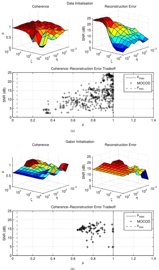
Figure 1 depicts the results of our experiment using re-spectively randomly chosen data from the training set and a twice over-complete Gabor dictionary for the initialisation. We run the experiment 5 times to increase the significance of our results whenever the initialisation involved choosing a random subset of the training data as the initial dictionary.
When ζ →0 andη → ∞, the optimisation (6) converges to a standard dictionary learning where the atoms are not forced to be incoherent, but are constrained to be unit norm. This case corresponds to the left corner of the surf plots in Figure 1. We can note that a data initialisation produces a highly coherent dictionary with the best approximation quality, while a Gabor initialisation results in a lower coherence at the expense of a worse SNR. Continuing our analysis in the case of data initialisation, keepingη → ∞and increasing the coherence penalty factor ζ results in a dictionary with lower mutual coherence, but also in a worse approximation quality. This behaviour is further illustrated by the mutual coherence-reconstruction scatter plot, which depictsµagainstSNRof the sparse approximation for every learned dictionary and exhibits a clear (although highly variable) trend. In the case of Gabor initialisation, on the other hand, it seems that the parameter
ζ does not affect mutual coherence and reconstruction error for high values ofη, while decreasing the penalty factorηhas generally a negative effect on both µandSNR of the learned dictionaries.
To understand the poor performance of the MOCOD algo-rithm, especially when initialised with a Gabor dictionary, we inspected µ and SNR of the sparse approximation at every iteration, along with the percentage change of the dictionary with respect to the Frobenious norm, that is defined as:
100 Φ(t+1)−Φ(t) F Φ(t) F (14) were Φ(t) indicates the dictionary at iterationt.
The main observation that underlies the poor performance
ofMOCODis that the percentage change of the dictionary does not converge to zero as the number of iterations increases and, therefore, the algorithm does not converge to a fixed point of the objective function (6). Wheneverη is set to be small (that is, when the dictionary atoms are not forced to be unit norm), the optimisation is very unstable and we often observed that the mutual coherence ends being greater than the one of the initial dictionary, especially for low values ofζ.
When η is set to be large, the algorithm still does not converge to a fixed point of the objective function, but the mutual coherence and SNR are much more stable. In this case different initialisations lead to different solution paths as evaluated in terms of SNR and mutual coherence as a function of the optimisation iterations. In the case of data
initialisation, the mutual coherence drops and the SNR oscil-lates, while in the case ofGabor initialisation, the SNRdoes not change significantly and the mutual coherence slightly increases. Moreover, the minimum mutual coherence achieved byMOCODin the results shown is never smaller than0.3, and further experiments with penalisation terms η = ζ = 1010
confirmed that the algorithm is unable to reach lower mutual coherence levels.
Unlike MOCOD, INK-SVD and the proposed IPR algorithm allow us to set a target coherenceµ0and to run the dictionary
decorrelation iteratively until it is achieved.
B. IPRand INK-SVD
After experimenting with different combinations of dictio-nary learning and decorrelation iteration numbers, we found that consistently good results can be achieved by performing
50iterations of theK-SVD dictionary learning combined with
5iterations of the relevant decorrelation method. This also led to comparable running times, as will be discussed in Section IV-C. We set the target mutual coherence in logarithmically spaced intervals from 0.05 to1 and compared the two algo-rithms by evaluating the achieved SNR. When applying the methods to an initial dictionary formed by randomly selected vectors from the training set, we run the experiment for 10 independent trials to obtain more significant results.
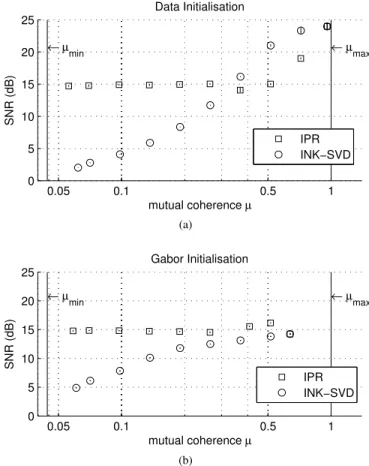
Figure 2 depicts the results of our experiment. As can be noted, both algorithms succeed in matching the target coherence levels for both initialisations except for the lower end on the left side of the plots, withIPRperforming slightly better in achieving the smallest mutual coherence in the case of data initialisation, reaching a value of around0.055compared to the0.06of INK-SVD. Whenever the target coherenceµ0 is
larger than the coherence level achieved without dictionary de-correlation, the two methods simply act as a K-SVD without any mutual coherence constraint. In the case of data initial-isation, we can observe that INK-SVD obtains a good SNR
10−2 100 102 104 10−2 100 102 104 0 0.5 1 η Coherence ζ µ 10−2 100 102 104 10−2 100 102 104 0 5 10 15 20 25 η Reconstruction Error ζ SNR (dB) 0 0.2 0.4 0.6 0.8 1 1.2 1.4 0 5 10 15 20 25 µ SNR (dB)
Coherence−Reconstruction Error Tradeoff
µmax MOCOD µmin Data Initialisation (a) 10−2 100 102 104 10−2 100 102 104 0 0.5 1 η Coherence ζ µ 10−2 100 102 104 10−2 100 102 104 0 5 10 15 20 25 η Reconstruction Error ζ SNR (dB) 0 0.2 0.4 0.6 0.8 1 1.2 1.4 0 5 10 15 20 25 µ SNR (dB)
Coherence−Reconstruction Error Tradeoff
µ max MOCOD µ min Gabor Initialisation (b)
Figure 1: Mutual coherence and reconstruction error achieved using the MOCOD dictionary update and (a) randomly chosen samples from the training set or (b) a Gabor frame as the initial dictionary. The surf plots show the mutual coherence andSNR of the sparse approximation as a function of the two regularisation parametersη andζin equation (6). In the scatter plots, the levels µmax= 1andµmin=
p
(K−N)/N(K−1)indicate the maximum and minimum coherence attainable by a N×K
0.05 0.1 0.5 1 0 5 10 15 20 25 mutual coherence µ SNR (dB) Data Initialisation ← µmin ← µmax IPR INK−SVD (a) 0.05 0.1 0.5 1 0 5 10 15 20 25 mutual coherence µ SNR (dB) Gabor Initialisation ←µmin ←µmax IPR INK−SVD (b)
Figure 2: Mutual coherence and reconstruction error achieved using the proposed iterative projections and rotations (IPR) algorithm and INK-SVD dictionary decorrelation, initialised with (a) randomly chosen samples from the training set as the initial dictionary or (b) a twice over-complete Gabor dic-tionary. The error bars in (a) represent the standard deviation resulting from 10 independent trials of the experiment and indicate that the results are consistent, regardless the random element introduced in the initialisation.
for mutual coherence values greater than µ= 0.3, after that its performance degrades substantially. On the contrary, the proposed IPR does not perform as well for high coherence values, but does not significantly degrade from µ = 0.3 to
µ = 0.05. The results for Gabor initialisation, on the other hand, favour the proposed algorithm showing a better SNR and no significant approximation degradation for all the target coherence values.
It is worth noting that using theIPRalgorithm both data and Gabor initialisations lead to incoherent dictionaries producing similar SNR values. This suggests that the algorithm might converge to equivalent fixed points of the optimisation function regardless of its initialisation. Despite this being a desirable result, we cannot claim it to be a general property of the IPR algorithm, as we would require a formal analysis of the convergence of dictionary learning that is outside the scope of the present paper. On the other hand, the particular SNR value of about 15dB reached by the optimisation depends on the training set used to learn the dictionary, as will be sown in Section IV-D that presents results obtained with a different
0.05 0.1 0.5 1 0 100 200 300 mutual coherence µ time (s) Data Initialisation ← µmin ← µmax IPR INK−SVD (a) 0.05 0.1 0.5 1 0 100 200 300 mutual coherence µ time (s) Gabor Initialisation ←µmin ←µmax IPR INK−SVD (b)
Figure 3: Running times of IPR and INK-SVD for different mutual coherence levels and dictionaries initialised with (a) randomly chosen samples from the training set or (b) a twice over-complete Gabor dictionary. The error bars indicate the standard deviation resulting from 10 independent trials of the experiments.
training set.
C. Running times
Figure 3 shows the running times of the IPR and INK-SVD algorithms for different coherence levels, tested on a iMac with a 3.06GHz Intel Core 2 Duo processor running MATLAB R2011a and thecputimefunction. TheIPRvalues are not dependant on the coherence level and are just below
100 seconds, whereasINK-SVD takes longer to compute less coherent dictionaries. This is because INK-SVD acts in a greedy fashion by decorrelating pair of atoms until the target mutual coherence is reached (or until a maximum number of iterations) and therefore the number of pairs of atoms to decorrelate increases for low values of the target coherence.
The time required to compute a non de-correlated dictionary can be found in the right end of the plots and is around 20
seconds, which is also consistent with the average time of23
seconds needed by theMOCODalgorithm. This means that the cost ofIPRis about 5times the cost of a standardK-SVD for the problem sizes considered in our experiments.
D. Sparse approximation results
The relation between the coherence of a dictionary and its approximation properties for different classes of signals is a complex topic. In this section we do not attempt a formal convergence analysis of the tested dictionary learning algorithms as this is outside the scope of the present paper.
The trade-off between mutual coherence and SNR of the sparse approximation visible in Figures 1a, 2a and 2b is consistent with the fact that the different decorrelation methods aim at solving penalised or constrained optimisation problems. If we compare the general dictionary learning problem intro-duced in Section I-A to the incoherent formulations presented in this paper, the penalty factors used to promote incoherence in the unconstrained optimisation (6) and the feasible set con-sisting of dictionaries with bounded mutual coherence in the constrained problem (9) suggest that an incoherent dictionary is expected to have a worse approximation performance if compared to a coherent one. On the other hand, dictionary learning is a non-convex optimisation problem that to the best of our knowledge lacks strong and general convergence results, relying instead on the ability of practical algorithms to converge to local minima of the optimisation cost function. For the purpose of the experimental evaluation of the IPR algorithm, we tested whether the mutual coherence versus SNRtrade-off is consistent over different training and testing signals. We considered the following test material:
• music03_16kHz, a guitar recording distributed as part of the SMALLBOXthat was used to train the dictionaries in the experiments presented so far.
• track n.6 of the jazz section of the RWC music
database3, which is an electric guitar recording.
• track n.1 of the jazz section of the RWC music
database, which is an acoustic piano recording.
After running the IPR dictionary learning algorithm on the guitar recording track n.6 using the data initialisation, the same problem parameters specified in Section IV and the target mutual coherence levels specified in Section IV-B, we employed the learned dictionaries to approximate the two remaining test signals, using the OMP algorithm and 5% of active atoms, as in the learning phase.
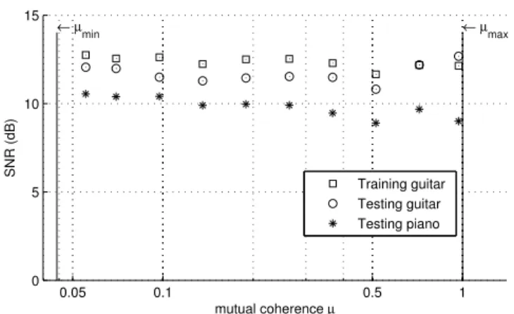
Figure 4 displays the results of the experiment. If we compare these values to the ones presented in Figure 2a, we can note that the trade-off between mutual coherence and SNR is no longer present, and that the approximation of the training set (which in the case of the training guitar is inversely proportional to the residual norm in the cost function (9)) is around 12 and 13 dB for the two guitar signals and around 10 dB for the piano signal. The absence of a steep peak in correspondence with a dictionary with high mutual coherence and the overall worse approximation performance can be explained by the fact that music03_16kHz is a relatively short signal, that as a consequence when learning a dictionary from this signal the number of training vectors compared to the size of the dictionary is relatively low and that we observed a few signals that could be approximated very well using only one atom in the dictionary. This does not happen when learning a dictionary from a longer training set obtained using track n.6 and results in overall worse but more consistent results.
3available at http://staff.aist.go.jp/m.goto/RWC-MDB/ 0.05 0.1 0.5 1 0 5 10 15 ←µmin ←µmax mutual coherence µ SNR (dB) Training guitar Testing guitar Testing piano
Figure 4: Mutual coherence versusSNRof the sparse approx-imation using a dictionary learned fromtrack n.6 of the jazz section of theRWCdatabase using data initialisation,OMP and5%of active atoms in the sparse coding step of dictionary learning. In the testing phase, OMP with5% of active atoms was also used to approximate signals from the training set,
from music03_16kHz that is a different guitar recording
and formtrack n.1of the jazz section of theRWCdatabase that is a piano recording.
V. CONCLUSIONS AND PLANS FOR FUTURE INVESTIGATION
We presented the iterative projections and rotations (IPR) decorrelation algorithm, a method for dictionary decorrelation to be used within the context of dictionary learning. Our technique is based on an iterative projection optimisation used to construct Grassmannian frames and includes a dictionary rotation step that makes it suitable for the approximation objective (9) of dictionary learning. Experiments on musical audio data demonstrate the performance of IPR and suggest that it can outperform state-of-the-art algorithms especially when a very low mutual coherence is required. The computa-tional time ofIPR is of the same order of magnitude than the time required by a standard K-SVD dictionary learning.
Exploring the applications of the proposed work is one of the main objectives for future investigation. On one hand, incoherent dictionary learning can be adapted and applied to compressed sensing technologies, both for audio and for other types of signals that are amenable to sparse approxima-tions. On the other hand, classification and separation tasks can benefit from the proposed algorithm in the context of morphological component analysis. IPR acts on the Gram matrix by thresholding the correlation between the atoms of the dictionary, and can be easily adapted to decorrelate only certain subsets of the dictionary that correspond to different morphological components or sources.
Finally, extending the decorrelation strategy to more accu-rate measures of coherence, such as the cumulative coherence proposed by Tropp [32], and a better theoretical understanding of the interplay between coherence and approximation perfor-mance are both objects of current endeavours.
REFERENCES
[1] M. Aharon, M. Elad, and A. Bruckstein. K-SVD: An algorithm for designing overcomplete dictionaries for sparse representation. IEEE Trans. on Signal Processing, 54(11):4311–4322, Nov. 2006.
[2] M. Aharon, M. Elad, and A. M. Bruckstein. On the uniqueness of overcomplete dictionaries, and a practical way to retrieve them.Linear Algebra and its Applications, 416(1):48–67, Jul. 2006.
[3] D. Barchiesi. Dictionary learning for the sparse approximation of audio signals. Research Open Day, School of Electronic Engineering and Computer Science, Queen Mary University of London, Apr. 2012. [4] T. Blumensath and M. E. Davies. Iterative thresholding for sparse
ap-proximations.Journal of Fourier Analysis and Applications, 14(5):629– 654, 2008.
[5] J. Bobin, Y. Moudden, and J.-L. Starck. Enhanced source separation by morphological component analysis. In Proceedings of the IEEE International Conference on Acoustics, Speech and Signal Processing (ICASSP), volume 5, pages 833–866, 2006.
[6] J. Bobin, J.-L. Starck, J. M. Fadili, Y. Moudden, and D. L. Donoho. Morphological component analysis: An adaptive thresholding strategy. IEEE Trans. on Image Processing, 16(11):2675–2681, Nov. 2007. [7] E. Candès and M. B. Wakin. An introduction to compressive sampling.
IEEE Signal Processing Magazine, 25(2):21–30, Mar. 2008.
[8] S. S. Chen, D. L. Donoho, and M. A. Sauders. Atomic decomposition by basis pursuit. SIAM Review, 43(1):129–159, Mar. 2001.
[9] W. Dai, T. Xu, and W. Wang. Dictionary learning and update based on simultaneous codeword optimization (SIMCO). InProceedings of the IEEE International Conference on Acoustics, Speech and Signal Processing (ICASSP), pages 2037–2040, 2012.
[10] I. Damnjanovic, M. E. P. Davies, and M. D. Plumbley. SMALLbox - An evaluation framework for sparse representations and dictionary learning algorithms. InProceedings of the International Conference on Latent Variable Analysis and Signal Separation (LVA/ICA), pages 418– 425, 2010.
[11] G. Davis, S. Mallat, and M. Avellaneda. Adaptive greedy approxima-tions. Constructive Approximation, 13(1):57–98, 1997.
[12] R. A. DeVore. Nonlinear approximation. Acta Numerica, 7:51–150, 1998.
[13] K. Engan, S. O. Aase, and J. H. Husøy. Method of optimal directions for frame design. InProceedings of the IEEE International Conference on Acoustics, Speech and Signal Processing (ICASSP), volume 5, pages 2443–2446, 1999.
[14] Q. Geng, H. Wang, and S. J. Wright. On the local cor-rectness of `1-minimization for dictionary learning. available at
http://arxiv.org/pdf/1101.5672.pdf, Feb. 2011.
[15] R. Gribonval and K. Schnass. Dictionary identification: Sparse matrix-factorisation via`1-minimisation. IEEE Trans. on Information Theory,
56(7):3523–3539, Jul. 2010.
[16] R. Gribonval and P. Vandergheynst. On the exponential convergence of matching pursuit in quasi-incoherent dictionaries. IEEE Trans. on Information Theory, 52(1):255–261, Jan. 2006.
[17] B. K. Horn, H. M. Hilden, and S. Negahdaripour. Closed-form solution of absolute orientation using orthonormal matrices. Journal of the Optical Society of America A, 5:1127–1135, July 1988.
[18] M. Lewicki and T. Sejnowski. Learning overcomplete representations. Neural Computation, 12(2):337–365, Feb. 2000.
[19] B. Mailhé, D. Barchiesi, and M. D. Plumbley. INK-SVD: Learning incoherent dictionaries for sparse representations. In Proceedings of the IEEE International Conference on Acoustics, Speech and Signal Processing (ICASSP), pages 3573–3576, 2012.
[20] B. Mailhé and M. D. Plumbley. Local optimality of dictionary learning algorithms. InProceedings of the Workshop on Signal Processing with Adaptive Sparse Structured Representations (SPARS), page 67, 2011. [21] J. Mairal, F. Bach, J. Ponce, and G. Sapiro. Online learning for matrix
factorization and sparse coding.Journal of Machine Learning Research, 11:19–60, Jan. 2010.
[22] S. Mallat and Z. Zhang. Matching pursuit with time-frequency dic-tionaries. IEEE Trans. on Signal Processing, 41(12):3397–3415, Dec. 1993.
[23] D. Needell and J. A. Tropp. CoSaMP: Iterative signal recovery from incomplete and inaccurate samples. Applied and Computational Harmonic Analysis, 26:301–321, 2008.
[24] D. Needell and R. Vershynin. Uniform uncertanty principle and signal recovery via regularized orthogonal matching pursuit. Foundations of Computational Mathematics, 9(3):317–334, 2009.
[25] Y. Pati, R. Rezaiifar, and P. Krishnaprasad. Orthogonal matching pursuit: Recursive function approximation with applications to wavelet decomposition. In Proceedings of the 27th Asilomar Confrence on Signals, Systems and Computers, volume 1, pages 40–44, Nov. 1993. [26] I. Ramírez, F. Lecumberry, and G. Sapiro. Sparse modeling with
universal priors and learned incoherent dictionaries. Technical Report 2279, Institute for Mathematics and its Applications, University of Minnesota, Sep. 2009.
[27] R. Rubinstein, A. Bruckstein, and M. Elad. Dictionaries for sparse representation modeling. Proceedings of the IEEE, 98(6):1045–1057, Jun. 2010.
[28] K. Schnass and P. Vandergheynst. Dictionary preconditioning for greedy algorithms. IEEE Trans. on Signal Processing, 56(5):1994–2002, May 2008.
[29] K. Skretting and K. Engan. Recursive least squares dictionary learning algorithm. IEEE Trans. on Signal Processing, 58(4):2121–2130, Apr. 2010.
[30] E. C. Smith and M. Lewicki. Efficient auditory coding. Nature, 439(23):978–982, Feb. 2006.
[31] T. Strohmer and R. W. J. Heath. Grassmannian frames with applications to coding and communication. Applied and Computational Harmonic Analysis, 14(3):257–275, 2003.
[32] J. A. Tropp. Greed is good: Algorithmic results for sparse approxi-mation. IEEE Trans. on Information Theory, 50(10):2231–2242, Oct. 2004.
[33] J. A. Tropp. On the conditioning of random subdictionaries. Applied and Computational Harmonic Analysis, 25(1):1–24, Jul. 2008. [34] J. A. Tropp, I. S. Dhillon, R. W. J. Heath, and T. Strohmer. Designing
structured tight frames via an alternating projection method.IEEE Trans. on Information Theory, 51(1):188–209, Jan. 2005.
[35] M. Yaghoobi, L. Daudet, and M. E. Davies. Parametric dictionary design for sparse coding.IEEE Trans. on Signal Processing, 57(12):4800–4810, Dec. 2009.
Mark D. Plumbley (S’88–M’90–SM’12) received the B.A. (Hons.) degree in electrical sciences in 1984 from the University of Cambridge, Cambridge, U.K., and the Ph.D. degree in neural networks in 1991, also from the University of Cambridge. From 1991 to 2001 he was a Lecturer at King’s College London. He moved to Queen Mary University of London in 2002, and where he is now an EPSRC Leadership Fellow and Director of the Centre for Digital Music. His research focuses on the automatic analysis of music and other audio sounds, including automatic music transcription, beat tracking, and audio source separation, and with interest in the use of techniques such as independent component analysis (ICA) and sparse representations. Prof. Plumbley is a member of the IEEE SPS TC on Audio and Acoustic Signal Processing.
Daniele Barchiesireceived the BSc degree in ap-plied mathematics in 2008 from Università di Roma Tor Vergata, Italy, the MSc by research degree in 2009 and the Ph.D. degree in electronic engineering in 2013 from Queen Mary University of London, U.K. He is now a post-doctoral research assistant at the Centre for Digital Music, Queen Mary University of London. His main research interests are on sparse approximation and dictionary learning with applica-tions to audio signals, audio scenes classification and audio events recognition. Dr. Barchiesi also worked on automatic mixing and reverse engineering of audio mixes for audio production applications.