Bayesian credibility for GLMs

Accepted Manuscript

Oscar Alberto Quijano Xacur, José Garrido

PII: S0167-6687(17)30413-4

DOI: https://doi.org/10.1016/j.insmatheco.2018.05.001 Reference: INSUMA 2463

To appear in: Insurance: Mathematics and Economics Received date : September 2017

Revised date : January 2018 Accepted date : 9 May 2018

Please cite this article as: Xacur O.A.Q., Garrido J., Bayesian credibility for GLMs.Insurance: Mathematics and Economics(2018), https://doi.org/10.1016/j.insmatheco.2018.05.001

This is a PDF file of an unedited manuscript that has been accepted for publication. As a service to our customers we are providing this early version of the manuscript. The manuscript will undergo copyediting, typesetting, and review of the resulting proof before it is published in its final form. Please note that during the production process errors may be discovered which could affect the content, and all legal disclaimers that apply to the journal pertain.

Bayesian Credibility for GLMs

Oscar Alberto Quijano Xacur

and Jos´e Garrido

Concordia University, Montreal, Canada

January 20, 2018

Dedicated to the memory of Bent Jørgensen;

a true scholar, a gentlemen and a great person.

Abstract

We revisit the classical credibility results of Jewell [8] and B¨uhlmann [2] to obtain credibility premiums for a GLM using a modern Bayesian approach. Here the prior distribution can be chosen without restric-tions to be conjugate to the response distribution. It can even come from out–of–sample information if the actuary prefers.

Then we use the relative entropy between the “true” and the es-timated models as a loss function, without restricting credibility pre-miums to be linear. A numerical illustration on real data shows the feasibility of the approach, now that computing power is cheap, and simulations software readily available.

1

Introduction

The well known classical result from Jewell [8] gives exact linear cred-ibility estimators for the exponential family. More precisely, it applies to random variables Y with distribution in some exponential disper-sion family (EDF), i.e. with density

∗_{Corresponding author: [email protected]. The authors gratefully}

f(y|θ, φ) =a(y, φ) exp 1 φ{yθ−κ(θ)} , θ∈Θ, φ∈Φ. (1) Assuming that φ is known, Jewell uses the following prior density on

θ:

πn0,x0(θ)∝exp n0[x0θ−κ(θ)]

, (2)

for some hyper–parameters n0 > 0 and x0 in the support of Y. For

a conditionally i.i.d. sample y1, . . . , yn of Y, given θ, Jewell showed

that the marginal mean ofY given this sample is

E[Y_|y1. . . yn] = φn0 φn0+nx0+ n φn0+ny¯ (3) = (1−z)x0+zy,¯

where ¯y= _n1Pn_i=1yiandz= _φnn_0+n is known as the credibility factor.

Note that (3) is the B¨uhlmann [2] Bayesian point estimator of the mean of Y that minimizes the expected square loss error and it is known as the linear credibility estimator.

The purpose of this article is to present a methodology for obtain-ing credibility estimators that generalize these ideas and allow them to be applicable to Generalized Linear Models (GLMs).

Hachemeister [7] and De Vylder [5] give classical credibility results for regression models. The main idea in these articles is similar to B¨uhlman’s: they first impose linearity on the regression covariates and then find the optimal linear parameter estimators by minimizing a distance or error function.

Nelder and Verall [17] and Ohlsson [18] propose linear credibility estimators for GLMs. Although different in substance, these two ar-ticles have in common that they are both likelihood based and both rely on random effects in order to obtain credibility estimates. The resulting Generalized Linear Mixed Models (GLMMs) credibility pre-miums remain essentially linear, which differs fundamentally from the method proposed here.

In this article we use a modern Bayesian approach to obtain cred-ibility estimators. We focus on extending Jewell’s results to General-ized Linear Models (GLMs). Our estimator is not linear as we do not impose linearity constraints, nor force the prior to be conjugate. It also offers the advantage of considering the uncertainty on the disper-sion parameter.

The exposition is divided as follows. In Section 2 we review the es-sential elements needed to introduce our estimator. Section 3 presents entropic estimators and some properties of the unit deviance that are important for the rest of the article. In Section 4 we discuss the un– feasibility of exact linear credibility for GLMs. Section 5 proves that it is possible to obtain entropic estimators for GLMs, which is our proposed credibility approach. Moreover, Proposition 5.1 suggests an algorithm to obtain the estimators.

Finally, in Section 6 we show that our method is applicable to real life datasets by fitting the model to a publicly available dataset. A commented version of the R code used for this can be found at

https://oquijano.net/articles/bayesian_credibility/.

2

Preliminaries

2.1

Exponential Dispersion Families

In (1)θand Θ are called the canonical parameter and canonical space, respectively and φ is known as the dispersion parameter. A neat property of reproductive exponential families is that for θ _∈ int (Θ) (here int stands for interior),

E[Y] = ˙κ(θ) and V[Y] =φκ¨(θ), (4) where ˙κ=κ0 and ¨κ= ˙κ0. This motivates the following definitions.

Definition 2.1. Given an exponential dispersion family, the mean domain of the family is defined as

Ω =_{µ= ˙κ(θ) :θ_∈int(Θ)_}.

Another important property is that the support of the distribution only depends on φ (and not on θ). For a given family, let Cφ be the

convex support of any member of the family with dispersion parameter

φ. We define the convex support of the family as

CΦ= [

φ∈Φ Cφ.

Definition 2.2. The unit deviance function of an exponential

disper-sion family is defined as d:CΦ×Ω→[0,∞) with

d(y, µ) = 2 sup θ∈Θ{ θy₋κ(θ)_{} −}yκ˙−1(µ) +κ κ˙−1(µ) . (5)

The unit deviance function plays an important role in the theory of GLMs. The model assessment of a GLM is through hypothesis tests that are based on the asymptotic behaviour of the unit deviance function. It also allows to re-parametrize (1) as

f(y|µ, φ) =c(y, φ) exp − 1 2φd(y, µ) . (6)

This is known as the mean–value parameterization and it is the one used in this article.

When the canonical space Θ is open, it is said that the EDF is regular. In this caseCΦ= Ω and (5) is equivalent to

d(y, µ) = 2y{κ˙−1(y)−κ˙−1(µ)} −κ κ˙−1(y)+κ κ˙−1(µ). (7) In the rest of the article we work with regular EDFs. Notice that all the usual distributions used for GLMs are regular (e.g. all the distributions in the Tweedie family are regular).

There is a useful property of reproductive exponential dispersion families that allows for data aggregation. Jørgensen’s notation (from [11]) is very convenient to express this property: given a fixed ex-ponential family, if Y has mean µ and density given by (6), we say that it is ED(µ, φ/w) distributed. The property is then as follows: if

Y1, Y2,· · ·, Yn are independent, andYi∼ED(µ, φ/wi), then

¯ Y = w1Y1+· · ·+wnYn w+ ∼ED(µ, φ/w+), w+= n X i=1 wi. (8)

2.1.1

A Note on Aggregating Discrete Exponential

Dis-persion Models

There are two usual parametrizations of exponential dispersion fami-lies. (1) gives the density ofreproductive EDFs and it is used for con-tinuous distributions. Discrete distributions are usually parametrized

as additive EDFs, whose densities have the form

f(y_|θ, φ) =a(y, φ) exp yθ₋ 1 φκ(θ) , θ_∈Θ, φ_∈Φ. (9) Both parametrizations are defined and discussed in Jørgensen [11] and Jørgensen [10]. GLMs assume the reproductive parameterization (see Nelder and Wedderburn [16]). Now, for many discrete EDFs, the

dispersion parameter has a known value. Specifically, for the Poisson, Bernoulli and negative binomial distributions φ = 1. This makes (1) and (9) the same parametrization and allows such distributions to enter the GLMs framework. Nevertheless, it is important to be aware that for the discrete case, one cannot aggregate data using (8). The properties of the Poisson distribution allow to use an offset for data aggregation (see for example Section 9.5 of Kaas, Goovaerts et al. [12]). Other discrete distributions can be aggregated using quasi-likelihood.

2.2

Relative Entropy

Let mi be probability measures with dmi(y) = fi(y)ds(y) for some

density functions f1, f2 and some probability measure s, withm1 ≡ m2 ≡s (that ism1, m2 ands are absolutely continuous with respect

to each other).

Definition 2.3. The relative entropy ofm2 fromm1 is defined as D(m1 km2) =Em1 log f1(Y) f2(Y) = Z log f1(y) f2(y) dm1(y).

This definition was introduced by Kullback and Leibler in [14].

D(· k ·) is often called the Kullback–Leibler divergence, nevertheless we prefer the term relative entropy since what they called divergence between m1 andm2 was D(m1km2) +D(m2km1).

The relative entropy is a measure of information. As such, it sat-isfies the invariance property. Intuitively this means that bijective transformations do not increase or decrease the information. The fol-lowing paragraph expresses this formally.

Let (Ω1,F, mi) and (Ω2,G, νi), for i = 1,2, be probability spaces

and T : Ω1 → Ω2 a measurable transformation such that νi(G) =

mi(T−1(G)), for G ∈ G. Define also γ(G) = s(T−1(G)). Since

m1 ≡ m2≡ s, then ν1 ≡ν2 ≡γ. This implies, by Radon–Nykodim’s

theorem that there existg1 andg2 such that νi(G) =

Z

G

gi(y)dγ(y), G∈ G.

With these definitions in mind, the following theorem asserts the in-variance property of the relative entropy. Its proof can be found in Chapter 2 of Kullback [13].

Theorem 2.1. D(m1 k m2) = D(ν1 k ν2) if and only if T is a

bijective transformation.

2.3

GLMs

In a GLM the response variable is assumed to follow a EDF with density f(y|θ, φ) =a(y, φ) exp w φ{yθ−κ(θ)} , (10)

Note thatφ in (1) corresponds toφ/w in (10) which implies that the mean and variance can be expressed asµ=κ0(θ) andσ2 _=φκ00_(θ)/w,

respectively. Here w _≥0 is know as the weight. In applications w is known usually andφneeds to be estimated. It is further assumed that there is a vector of explanatory variables, also known as covariates,

x = (x1· · ·xp)T, a vector of coefficients β = (β0 β1· · ·βp)T and a

function gknown as the link function such that

g(µ) =β0+x1β1+· · ·+xpβp. (11)

It is useful for further developments to express the canonical parameter

θ in terms of the coefficients. Sinceµ=κ0_{(θ)≡κ˙(θ) then:}

(g◦κ˙)(θ) =β0+x1β1+· · ·+xpβp

θ= (g◦κ˙)−1(β0+x1β1+· · ·+xpβp). (12)

The population can be divided into different classes according to the values of the explanatory variables. Thus, given a sample, we can group together all the observations that share the same values of the explanatory variables and aggregate them using (8). It is important to mention that with this grouping there is no loss of information for estimating the mean since ¯Y is a sufficient statistic forθ (but not for

φ, thus some information is lost for the estimation ofφ).

Possibly after aggregating, let m be the number of classes and

θ_∈Θm_{, where Θ}m_=(θ

1· · ·θm)T :θ1, . . . , θm∈Θ . The density of

the sample can be expressed as

f(y_|θ, φ) =A(y, φ) exp yTWθ−1TWκ(θ) φ , y_∈Rm, (13)

where κ(θ) = κ(θ1)· · ·κ(θm)T, W = diag(w1,· · ·, wm), with wi

A(y, φ) = Qm_i=1 a(yi,w_φi). In order to express θ in terms of β, we

define the following maps

µ=κ˙(θ) =    ˙ κ(θ1) .. . ˙ κ(θm)   , G(µ) =G    µ1 .. . µm   =    g(µ1) .. . g(µm)   ,

and the design matrix

X =    1 xT 1 .. . 1 xT m   ,

wherexiis the vector of explanatory variables for thei-th class. Along

this article we assume thatX has full rank and that the model is not saturated (i.e. p+ 1< m). With all these definitions, we have that

G(µ) =Xβ,

(G◦κ˙)(θ) =Xβ,

θ= (G◦κ˙)−1(Xβ). (14) It is useful to reparameterize (13) in terms of the mean vector µ

instead of θ. Using the mean value parameterization (this is (6) but substituting φ forφ/w), (13) can be reparameterized as

f(y_|µ, φ) =C(y, φ) exp

−₂1_φD(y,µ)

, (15)

whereC(y, φ) =Qm_i=1c(yi,_wφ_i), andD: Ωm×Ωm→[0,∞) with

D(y,µ) =

m

X

i=1

wid(yi, µi), (16)

where Ωm=(µ1· · ·µm)T :µ1, . . . , µm∈Ω . Dis called the deviance

of the model. We give here some of its properties:

• Given a sample, finding the mle ofθ is equivalent to finding the value ofβ that minimizes the deviance.

• D can be used to estimate the dispersion parameter (although it is not the only method). The deviance estimator ofφ is given by

ˆ

φ= D(y,µˆ)

• The asymptotic distribution of D plays an important role in model assessment and variable selection.

For further details about the use and properties of the deviance we recommend Jørgensen [10].

3

Entropic Estimator

A posterior distribution is more informative than a point estimation since it reflects our uncertainty about the true parameter. Now, in insurance, it is necessary to charge a premium, which is a point esti-mate. In this section we define the point estimators that we propose as credibility premiums.

Consider a parametric family of distributions with a parameter θ

to be estimated. Assume thatθ0 is the “true” parameter. In Bayesian

point estimation one first chooses a loss function_L(θ0,θ1) that

repre-sents the cost of estimatingθ to beθ1 instead ofθ0. Now, sinceθ0 is

not known, we define a risk function as

R(θ) =_E[_L(θ0,θ)],

where the expectation is taken with respect to the posterior distri-bution of θ. Then the point estimator ˆθ of θ0 is the value of θ that

minimizes R. That is: ˆ

θ= argmin

θ R

(θ).

The entropic estimator is defined as the Bayesian point estimator when the loss function _L is the relative entropy of the distribution with the real parameterθ0 over the estimated one.

More precisely, assume that the density of a random vector Y

depends on a parameter θ. Denote with f(Y_|θ1) the density of Y

when θ takes some valueθ1. The loss function is defined as L(θ0,θ) =Eθ0 log f(Y|θ0) f(Y_|θ) .

The corresponding risk function is then defined as

R(θ) =E log f(Y_|θ0) f(Y|θ) :=Eπ Eθ0 log f(Y_|θ0) f(Y|θ) ,

where _Eπ is the expectation taken with respect to the posterior

Definition 3.1. The entropic estimator is defined as ˆ θ= argmin θ E log f(Y|θ0) f(Y_|θ) ,

where the expectation is taken with respect to the posterior distribution

of θ.

Consider θ to be the parameter of some model and let β = g(θ) be a bijective transformation. Entropic estimators have the appealing invariance property that if θ∗ is the entropic estimator of θ, then

β∗ _{= g(θ}∗_{) is the entropic estimator of β. This property is called}

invariance (this terminology is consistent with Bernardo [1]) .

Not all estimators have this property. For example the estimator that minimizes the square loss error, i.e. the posterior mean, is not in-variant. On the other hand, it is well known that maximum likelihood estimators are invariant.

3.1

Entropic Estimators for univariate EDFs

A key part of this article is to show how to find entropic estimators for GLMs. This is done in Section 4. In the rest of this section, we focus on entropic estimators for univariate EDFs and their relation to linear credibility. The main result of the section is Proposition 3.1, which is preceded by two technical lemmas that show properties of the unit deviance that are fundamental for finding entropic estimators of exponential families and GLMs (see the appendix for the proofs of these lemmas).

Lemma 3.1. Let d be the unit deviance of a univariate EDF in (5).

Then, there exist functionsd1 andd2 such that for(y, µ)∈Ω×Ω, we

have the following decomposition:

d(y, µ) =d1(y) +d2(y, µ). (17)

Moreover, d2 has the property that if Y is a random variable with

support in Ω, andµ is fixed, then

Ed2(Y, µ)=d2 E[Y], µ. Lemma 3.2. Lety be fixed, then

1. the value ofµthat minimizes d2(y, µ) is the same one that

2. d2(y, µ) is minimized when µ=y.

Table 1 shows d, d1 and d2 for the normal, Poisson and gamma

distributions.

Distribution d(y, µ) d1(y) d2(y, µ)

Normal (y−µ)2 _y2 _µ2_−2yµ

Poisson 2nylog_µy−(y−µ)o 2y[log(y)−1] 2 [µ−ylog(µ)] Gamma 2nlogµ_y+_µy−1o 2h_µy + log(µ)i 2h_µy + logµ_y−1i

Table 1: Deviance decomposition of some common

EDF’s

Proposition 3.1. LetY be a random variable whose density is given

by (6) for some unknown values of µand φ,π(µ, φ) be a prior

distri-bution for (µ, φ), the vector y = (y1. . . yn)T be a conditionally i.i.d.

sample given (µ, φ), and π(µ, φ_|y) the corresponding posterior. The

entropic estimator µˆ of µis then given by

ˆ

µ=_E[Y_|y] =_EπEµ,φ[Y],

whereEπrepresents the expectation with respect to the posterior

distri-bution and Eµ,φ represent the expectations with respect to fixed values

of (µ, φ).

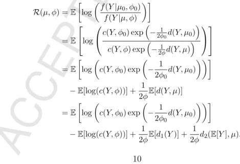
Proof. Let (µ0, φ0) be the true parameters. By Lemma 3.1, the

en-tropic risk measure can be expressed as

R(µ, φ) =_E log f(Y|µ0, φ0) f(Y_|µ, φ) =_E  log  c(Y, φ0) exp − 1 2φ0d(Y, µ0) c(Y, φ) exp−1 2φd(Y, µ)     =E log c(Y, φ0) exp −₂1_φ 0 d(Y, µ0) −E[log(c(Y, φ))] + 1 2φE[d(Y, µ)] =E log c(Y, φ0) exp −₂1_φ 0d(Y, µ0) −E[log(c(Y, φ))] + 1 2φE[d1(Y)] + 1 2φd2(E[Y], µ).

Note that, regardless of the value of φ, the value of µthat minimizes the expression above is the same one that minimizes the simpler func-tion

R1(µ) =d2 E[Y], µ.

Then, by Part 2 of Lemma 3.2, the entropic estimator of µis given by ˆ

µ=_E[Y].

This result shows that for univariate EDFs the posterior mean not only minimizes the expected square error risk, but also the posterior entropic risk. In the following sections we will see that this property does not generalize to GLMs due to the difference of dimension be-tween the response vector and the regression coefficients. For now, realize that a direct consequence of Proposition 3.1 is that Jewell’s estimator in [8] is an entropic estimator.

Corollary 3.1. The linear credibility estimator (3) is the entropic

estimator when φ is assumed known and (2) is used as prior forθ.

4

Linear Credibility for GLMs

This section discusses whether it is possible to extend Jewell’s result to GLMs. In other words we address the question: is there a prior for the regression coefficientsβfor which the posterior mean is a weighted mean between an out–of–sample estimate and the sample mean of a GLM?

There are two ways in which the question above can be interpreted. One could think of it as allmdimensions having the same credibility factor, that is, the credibility premium ˆµc is given by

ˆ

µc =zy¯+ (1−z)M, (18)

where ¯yis the GLM observed sample mean (i.e. a vector for which (8) applies to each coordinate),M is a vector of out–of–sample “manual” premiums as coordinates and z ∈ (0,1) is the credibility factor. We call this interpretation Linear Credibility of Type 1.

The other interpretation is to give a different credibility factor to each coordinate. This is

ˆ

µc =Zy¯+ (I−Z)M, (19)

where ˆµc, ¯y andM are as in (18), butZ = diag(z1, . . . , zm), wherezi

We call this interpretation Linear Credibility of Type 2. Note that linear credibility of Type 1 is a special case of linear credibility of Type 2.

4.1

Linear Credibility of Type 1 is Impossible

Jewell’s prior in (2) is a conjugate prior to (1) that gives linear credi-bility premiums based on the posterior mean. Diaconis and Ylvisaker [6] generalized Jewell’s result to multivariate exponential dispersion models. Since a GLM assumes that the response vector follows such a distribution, it could be conjectured that this automatically implies linear credibility for GLMs. In what follows we show that this is not the case.

After adapting the conjugate prior discussed in [6] to correspond to (13) so as to consider weights we get

πn0,x0(θ)∝exp n0{xT0Wθ−1TWk(θ)}

IΘm(θ), (20)

where n0 > 0, and x0 ∈ Ωm are the parameters of the prior

dis-tribution, Θm = (θ1. . . θm)T :θ1, . . . , θm∈Θ , IΘm is an indicator

function and Ωm _{= (µ}

1. . . µm)T :µ1, . . . , µm∈Ω . Theorem 3 of

[6] proves that if the support of (13) contains an interval then (20) is the only prior that gives linear credibility. This implies that for any continuous response (and also for any Tweedie distribution), (20) is the only prior that gives linear credibility. In the paper it is also proven that (20) is the unique prior that gives linear credibility for the binomial distribution and in Johnson [9] the same is proven for the Poisson distribution.

As shown in (14),θ andβare related byθ= ((G◦κ˙)−1◦X)(β). Thus, when a prior for βis chosen, a distribution is induced onθ. In what follows we refer to this distribution as the induced prior on θ. We have then that for continuous and Tweedie distribution and for the Poisson and negative binomial, a prior on the betas gives linear credibility if and only if the induced prior onθ is (20).

Our strategy to prove the impossibility of linear credibility of type 1 is to show that no prior of βinduces a prior on θ that has density (20). We can see that this is the case by focusing on the support of the induced distribution. Since the support of (20) is Θm, then it is enough to prove that the support of every induced prior of θ is different than Θm_.

Proposition 4.1. For any prior of β in a non-saturated GLM, the

support of the induced prior of θ is a proper subset of Θm.

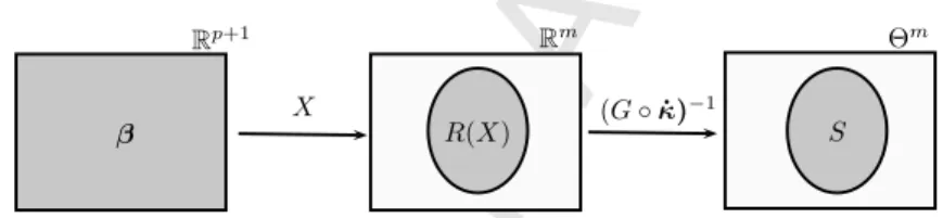
Proof. Since there is no restriction for the value ofβ, it can take any

value on _Rp+1_{. This is represented on the left rectangle of Figure 1.} Xβcan take values inR(X), whereR(X) is the range ofX. Since dim(R(X)) =p+ 1< m, thenR(X)( Rm. This is represented in the middle rectangle of Figure 1.

Let S be the support of the induced prior on θ. Then S _⊂ (G_◦ ˙

κ)−1_{(R(X)) :=(G◦κ˙)}−1_{(Xβ) :β∈R}p+1 _{(subset but not equality}

since some values of Rp+1 may not be in the support of β). Now, (G◦κ˙)−1 is a bijective function. Let p be a point in Rm that is not in R(X) and let q = (G◦κ˙)−1(p). Then q ∈ Θm but q ∈ S

because otherwise (G_◦κ˙)−1 _{would not be one-to-one. This proves}

that (G_◦κ˙)−1_(R(X))(Θm _{and therefore also thatS(Θ}m_{. This is}

represented in the right rectangle of Figure 1.

Rp+1

β R(X)

Rm _Θm

S

X (G◦κ˙)−1

Figure 1: From left to right the grey zone represents

the values that

β,

R

(

X

) and

S

can take, respectively.

Now, on a different but related note, it is possible to generalize (20) in a way that allows to obtain conjugate priors that are suitable for GLMs. Define

π1(θ)∝h(θ) exp n0{xT0Wθ−1TWk(θ)}

IΘm(θ),

wherehis some integrable function for which the integral on the right hand–side above is finite and denote this distribution byDconj(n0,x0). Proposition 4.2. π1 is a conjugate prior to (13) with posterior

dis-tribution Dconj

n0+_φ1,_n0φ1₊₁y¯+ _φnφn₀₊₁0 x0

.

Proof. Let π1(·|y) denote the posterior of π1. Then, by definition of

the posterior:

∝h(θ) exp n0xT0Wθ+ yT_Wθ φ −n01 T_Wk(θ)−1TWκ(θ) φ =h(θ) exp (n0xT0 + yT φ )Wθ− n0+ 1 φ Wκ(θ) =h(θ) exp  n0+ 1 φ _  n0xT0 + y T φ n0+ _φ1 Wθ₋1TWκ(θ)      =h(θ) exp n0+ 1 φ φn0xT0 +yT φn0+ 1 Wθ₋1TWκ(θ) ,

which proves the result.

Now, in order for π1 to overcome the problems that do not allow π in (20) to be used as a prior for GLMs, it is only necessary to chose

h such that π1 is outside of (G◦κ˙)−1(R(X)) with probability zero.

This way π1 has the “right” support and there is a distribution ofβ

that gives this distribution when transformed with ((G_◦κ˙)−1_◦X).

Two important remarks about π1:

1. It does not give linear credibility (since this is impossible as has been shown above).

2. It is not easy to find an analytic expression for µ (although this might be possible for some choices of π). Thus most likely one has to use some numerical method or MCMC in order to find the posterior means, but this defeats the purpose of using a conjugate prior.

4.2

Linear Credibility of Type 2 is Sometimes

Feasible

Since the model is a GLM, there should be a ˆβc such that ˆµc =

G−1(Xβˆc). Thus, (19) becomes

G−1(Xβˆc) =Zy¯+ (I−Z)M. (21)

It turns out that for non saturated models (i.e. dim(β)<dim(µ)), the existence of some ˆβc for which (21) can be satisfied depends on the

observed sample. We demonstrate why this is the case with a simple example in dimension 2.

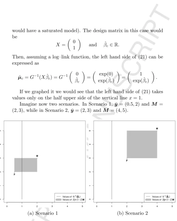
Consider a situation in which you divide your population in only 2 segments using a binary covariate with no intercept (otherwise we

would have a saturated model). The design matrix in this case would be X = 0 1 and βˆc ∈R.

Then, assuming a log–link function, the left hand side of (21) can be expressed as ˆ µc =G−1(Xβˆc) =G−1 0 ˆ βc = exp(0) exp( ˆβc) = 1 exp( ˆβc) .

If we graphed it we would see that the left hand side of (21) takes values only on the half upper side of the vertical linex= 1.

Imagine now two scenarios. In Scenario 1, ¯y = (0.5,2) and M = (2,3), while in Scenario 2, ¯y= (2,3) and M = (4,5).

(a) Scenario 1 (b) Scenario 2

Figure 2: Values of the left and right hand side of (21)

in both scenarios

As the values of the elements ofZ vary, the right hand side of (19) can take the values of the rectangle defined by ¯y and M. Figure 2 shows graphs with the possible values of the left and right hand side of (19) for each scenario.

In both graphs, the vertical line represents the values of ˆµc. The

take as the entries in the diagonal of Z vary from 0 to 1. In order to have exact linear credibility of type 2, it is necessary for the line and the rectangle to intersect. This is because the points of intersection, correspond to combinations of values ofβcandZfor which (21) holds.

If there is no intersection it is not possible to have linear credibility of type 2.

The graph of Scenario 1 shows that (19) is satisfied for some values ofZ, while in the graph for Scenario 2 it is impossible to satisfy (19). The results of this section show that Jewell’s result cannot be gen-eralized to GLM’s. That is, no prior for the parameters of a GLM guarantee linear credibility for all observed samples. In the next sec-tion we propose credibility estimators for GLMs that are not linear.

5

Entropic Credibility for GLMs

The Bayesian models proposed by B¨uhlmann and Jewell, using conju-gate priors that ensured linear credibility formulas, made great sense in the 1960’s and 70’s, when computational issues ruled out more gen-eral (non–linear) Bayesian solutions. However, computing power is no longer scarce nor expensive. In this section we propose a modern, computational Bayesian approach to credibility.

5.1

Estimation of the Mean

We propose an entropic estimator of the mean vector of a GLM as the credibility premium. This section focuses on how to find such an estimator. We start by enunciating the following technical lemma, which is an extension of Lemma 3.1 to greater dimensions. A proof can be found in the Appendix.

Lemma 5.1. LetDbe the deviance of a GLM (see (16)). Then there

exist functions D1 and D2 such that for(y,µ)∈Ωm×Ωm

D(y,µ) =D1(y) +D2(y,µ). (22)

Moreover, D2 has the property that if Y is a random vector with

sup-port in Ωm and µ∈Ωm is fixed, then

In what follows, an arbitrary prior π is assumed (not necessarily con-jugate) with posterior

π(β, φ_|y)_∝f(y_|β, φ)π(β, φ), (24) where f is as in (13) or, equivalently (15), depending on the chosen parameterization. As stated, _Eπ[·] denotes expectation with respect

to the posterior measure. Whenever the expectation symbol is used without a subindex, it means expectation with respect to the predic-tive posterior distribution, i.e.E[·] =Eπ[Eβ,φ(·)], whereEβ,φ(·) means

expectation with respect to the density in (13) with fixed coefficients vectorβand fixed dispersion parameter φ.

Proposition 5.1. The entropic estimator β∗ of the coefficients of a Bayesian GLM are equal to the maximum likelihood estimator of a frequentist GLM with the same covariates, response distribution and

weights, but with an observed response vector equal to _E[Y].

Proof. Let (β0, φ0) be the real parameters and (β, φ) some fixed

val-ues. We use here forf the mean value parameterization in (15). Then, the risk function is given by

R(β, φ) =Eπ{L[(β0, φ0),(β, φ)]}=E log f(Y_|µ0, φ0) f(Y|µ, φ) , whereµ=G−1_{(Xβ) andµ}

0=G−1(Xβ0). Then, by Lemma 5.1 and

(15) the expression above becomes

R(β, φ) =E log(C(Y, φ0))− 1 2φ0 D(Y,µ0) −E[log(C(Y, φ))] + 1 2φE[D(Y,µ)] =E log(C(Y, φ0))− 1 2φ0 D(Y,µ0) −E[log(C(Y, φ))] + 1 2φE[D1(Y) +D2(Y,µ)] =E log(C(Y, φ0))− 1 2φ0D(Y,µ0) + 1 2φD1(Y) −E[log(C(Y, φ))] + 1 2φE[D2(Y,µ)] =E log(C(Y, φ0))− 1 2φ0D(Y,µ0) + 1 2φD1(Y)

−E[log(C(Y, φ))] + 1

2φD2(E[Y],µ). (25)

The Bayesian point–estimator of (β0, φ0) is given by the vector (β∗, φ∗)

that minimizes R. Let us first focus on finding β∗. Note that this is equivalent to minimizing

R1(β) =D2(E[Y],µ). (26)

We first need to compute E[Y], which can be expressed as

E[Y] =EπEβ0,φ0[Y]

=EπG−1(Xβ).

Now, (24) gives π(·|y) up to a normalizing constant, thus the expec-tation above can be calculated with MCMC methods. In this way we consider the problem of computing _E[Y] solved.

Compare now the minimization of_R1(β) with a different

optimiza-tion problem for which the soluoptimiza-tion method is well known. Consider a frequentist (non–Bayesian) GLM with the same response distribu-tion, explanatory variables and weights. Imagine a sample under this model in which the observed response vector is equal to E[Y]. Using the mean value parameterization and Lemma 5.1, the log–likelihood function based on such a sample is given by

`(β, φ) = log(C(_E[Y], φ))₋ 1 2φD(E[Y],µ) = log(C(E[Y], φ))₋ 1 2φD1(E[Y])− 1 2φD2(E[Y],µ),

where µ = G−1(Xβ). Since the only term that depends on β is the third one, then maximizing `(β, φ) is equivalent to minimizing

D2(E[Y],µ), i.e. the same as minimizingR1(β). Hence, by obtaining

the mle of the regression coefficients of this hypothetical frequentist GLM, we obtain β∗ (or conclude that there is no solution, whenever this is the case).

Once β∗ has been found, the invariance property of the relative entropy allows to find the entropic premium straightforwardly.

Corollary 5.1. Ifβ∗ is the entropic estimator of the coefficients of a Bayesian GLM, then the entropic premium is given by

Remark 5.1. For a saturated model, i.e. when the dimension of β

is equal to the dimension of Y (in other wordsm =p), the entropic

premium is equal to E[Y]. This is because in a saturated model, the

predicted mean is equal to the observed response mean.

5.2

Estimation of the Dispersion Parameter

It is important to remark that the credibility estimator from the previ-ous section takes into consideration the uncertainty of the dispersion parameter. This is the case because the posterior distribution of β

depends on the posterior of φ.

This differs from classical credibility results where the dispersion parameter is considered known (e.g. Jewell [8] and Diaconis and Ylvisaker [6]). To the best of our knowledge there is only one article that consid-ers a prior distribution for the dispconsid-ersion parameter, Landsman and Makov [15], about which we have the following remarks:

1. The exponential distribution for the index parameter is justified using the principle of maximum entropy. The authors maximize the continuous entropy (that is entropy for continuous random variables), and use it for the index parameter assuming a known mean. Now, the continuous entropy does not have good proper-ties as a measure of information. For instance it is not invari-ant under bijective transformations, which implies that one can loose or gain information by just transforming a random vari-able. Thus, the principle of maximum entropy is not a valid justification for the exponential distribution. Nevertheless, it is a valid prior and one can use it in those cases where it reflects properly the out of sample information.

2. A more serious problem exists with the result in Theorem 2; the integrals in (7) are carried out assuming that λ is exponential with meanλ0. In other words, these are computed assuming the

prior distribution forλ. This is erroneous since it is the posterior distribution that should be used in this integral. This would be justified if the prior forλwere natural conjugate. In this way the posterior of λ would also be exponential, but the parameter of the posterior would be different than the parameter of the prior, in this case.

We have not found a general procedure for obtaining the entropic estimator of the dispersion parameter. We discuss here the cases for

which it can be found and present the difficulties in obtaining a general solution. Notice that a point–estimator forφis not necessary to obtain the credibility premium (as seen in Section 5.1) or its uncertainty (which is measured by the posterior distribution).

Suppose that the credibility premiumµ∗ has been obtained. From (25), one can see that finding the entropic estimatorφ∗ of the disper-sion parameter is equivalent to minimizing

R2(φ) =−E[log(C(Y, φ))] +

1

2φE[D(Y,µ∗)], (28)

where µ∗ = G−1(Xβ∗). There are standard methods for minimizing univariate functions, but R2 is more difficult because the first

expec-tation in (28) depends on φ. We consider first a special case where this minimization is rather straightforward. This is when there exists a function H :Rm_{×R→Rsuch that}

−E[log(C(Y, φ))] =H(E[Y], φ), (29) for every φ. In this case the problem simplifies considerably because once _E[Y] and _E[D(Y,µ∗_{)] have been found (most likely by}

simula-tions), then it is possible to use standard methods to find φ∗, since (28) becomes

R2(φ) =H(E[Y], φ) + 1

2φE[D(Y,µ∗)], (30)

which is simple to evaluate.

A case worth mentioning when (29) occurs is when the response distribution is a proper dispersion model (see Jørgensen [11, Chap. 5]), i.e. when cin (6) can be decomposed as

c(y, φ) =d(y)e(φ), (31) for some functions d and e. Then, the first term on the right hand side of (28) becomes

−E[log(C(Y, φ))] =−E

"_m Y i=1 log c Yi, φ wi # =_−E "_m Y i=1 log d(Yi)e φ wi #

=₋ m X i=1 E[log(d(Yi))]− m X i=1 log e φ wi .

Since Pm_i=1E[log(d(Yi))] does not depend on φ, the problem reduces

to minimizing R3(φ) =− m X i=1 log e φ wi + 1 2φE[D(Y,µ ∗_)],

which can be done using standard optimization methods. Now, it is known that there are only three exponential dispersion models for which the factorization in (31) holds: the gamma, inverse Gaussian and normal distributions (this result is commented in Jørgensen [11, Chap. 5] and proven in Daniels [3]). Table 2 givese is for these three models.

Distribution

Normal

Gamma

Inverse Gaussian

e

(

φ

)

φ

e

Γ(

φ

)

φ

φ

Table 2:

e

(

φ

) for the three proper exponential

disper-sion families

Let us now consider the general case where (30) does not hold. Again MCMC methods can be helpful. Let Y1, . . . ,YN be N sim-ulations of Y from the posterior predictive distribution (superscripts are used sinceYiwas already defined to be the i-th entry of Y). Now

define ˜ RN(φ) =− 1 N N X i=1 log(C(Yi, φ)) + 1 2φN N X i=1 D(Yi,µ∗),

then, for every fixed φ

lim

N→∞

˜

RN(φ) =R2(φ) a.s.. (32)

Let ˜φN = argmin ˜RN(φ). Since ˜RN is simple to evaluate with a

computer, standard univariate optimization methods can be used to find ˜φN. The question now is whether ˜φN converges toφ∗ asN → ∞?

We have not found easy–to–check sufficient conditions that guarantee convergence, although the following theorem might be useful in some cases.

Proposition 5.2. If the convergence in (32)is uniform almost surely w.r.t. φ, then R2(φ∗) = lim N→∞ ˜ RN( ˜φN) a.s.

Proof. On the one hand we have that for everyn_∈N

R2(φ∗)≤ R2( ˜φn)

∴ R2(φ∗)≤lim inf

n R2( ˜φn).

On the other hand, let > 0, since ˜RN → R2 uniformly a.s., then

with probability one there exists M >0, such that for every n_≥M,

|R˜n( ˜φn)− R( ˜φn)|< .

By the definition of ˜φn,

˜

Rn( ˜φn)≤ Rn(φ∗), for alln∈N.

Then for everyn_≥N,

R2( ˜φn)− <Rn(φ∗), thus lim sup n R2( ˜φn)−≤lim supRn(φ ∗₎ ∴ lim sup n R2( ˜φn)−≤ R2(φ ∗_{) a.s.}

Since this is true for >0, this implies that lim sup n R2( ˜φn)≤ R2(φ ∗_), and therefore R2(φ∗) = lim n→∞R( ˜φn) a.s.

6

On the Applicability of the Entropic

Premium

The previous section showed how one can find the entropic premium of a GLM, theoretically. In this section we address its practicability. In other words, we address the following question: is entropic credibility feasible for real–life datasets?

From Proposition 5.1 and Corollary 5.1, we have that once the re-sponse distribution, explanatory variables and prior have been chosen, the following steps give the entropic premium:

1. Find E[Y] (see the paragraph preceding Proposition 5.1 for the definition of_E[Y]).

2. Fit a frequentist GLM with the same covariates, response distri-bution and weights, but with observed response vector equal to

E[Y]. This givesβ∗, the entropic estimator of the coefficients. 3. Find the entropic mean using (27).

Steps 2 and 3 are simple: one can perform these computations in R (see [19]) without major problems. The difficult part is Step 1. To the best of our knowledge, the simplest way to solve this problem is using Markov Chain Monte Carlo (MCMC). In the paragraphs that follow we give some recommendations on how to use this method.

It is important to consider that the greater m (the dimension of

E[Y]), the more demanding the computations (both in terms of mem-ory and CPU). Thus, it is very useful to first aggregate the data as in (8). This can drastically reducemand turn an infeasible computation into something manageable.

A continuous variable can make data aggregation useless, espe-cially when this happens with several different variables in the dataset. In such cases one should consider converting the support of these ables into intervals, hence transforming them into categorical vari-ables.

Using Bayesian methods for variable selection can be time con-suming. This is because one would need to run MCMC simulations for each combination of variables. A pragmatic approach to deal with this is to choose the variables using a frequentist GLM (which is much faster to fit). The resulting combination of variables can be used to build a starting model in the Bayesian case.

6.1

Illustrative Example

In this section we use the R interface to STAN (see [20]) to find an entropic credibility estimate of a severity model for a publicly avail-able dataset. The main purpose of this example is to show that it is feasible to obtain entropic credibility premiums. We leave out the discussion about the convergence of the MCMC and the goodness of fit of the model. The interested reader can find the commented R code used for this example at https://oquijano.net/articles/ bayesian_credibility/.

Variable name Description

veh_value

vehicle value, in $10,000s

exposure

0-1

clm

occurrence of claim (0 = no, 1 = yes)

numclaims

number of claims

claimcst0

claim amount (0 if no claim)

veh_body

vehicle body, coded as

BUS

CONVT = convertible

COUPE

HBACK = hatchback

HDTOP = hardtop

MCARA = motorized caravan

MIBUS = minibus

PANVN = panel van

RDSTR = roadster

SEDAN

STNWG = station wagon

TRUCK

UTE - utility

veh_age

age of vehicle: 1 (youngest), 2, 3, 4

gender

gender of driver: M, F

area

driver’s area of residence: A, B, C, D, E, F

agecat

driver’s age category: 1 (youngest), 2, 3, 4, 5, 6

Table 3: Vehicle insurance variables

67,856 one–year policies from 2004 or 2005. It can be downloaded from the companion site of the book: http://www.acst.mq.edu.au/ GLMsforInsuranceData, as the dataset called Car. Table 3 shows the description of the variables as provided at the website.

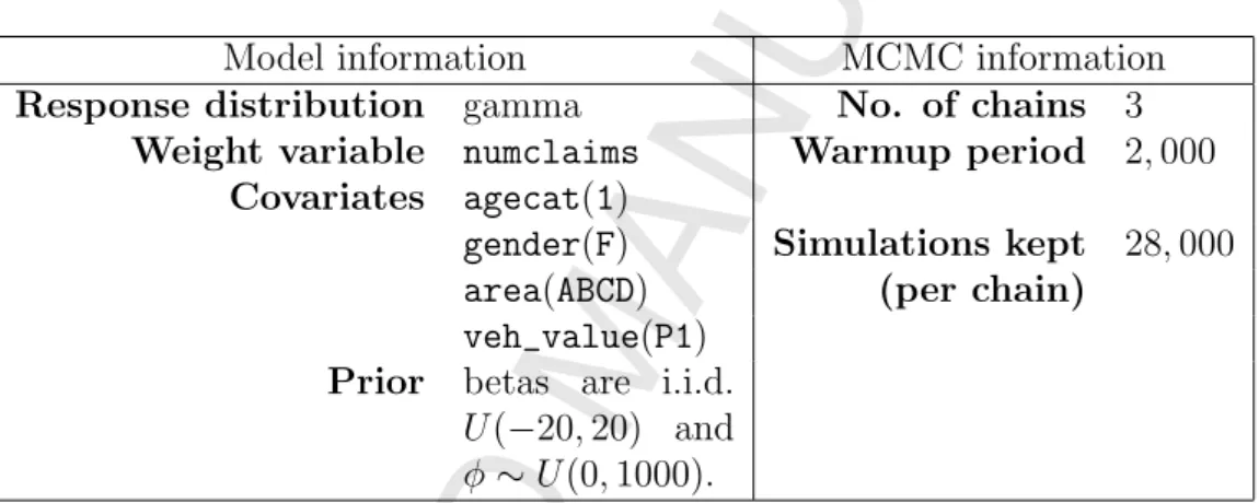
We use a GLM with gamma responses to model the severity (vari-able claimcst0). We modified two explanatory variables, dividing the support of the continuous variable veh_valueinto three intervals [0,1.2),[1.2,1.86) and [1.86,_∞), which we label asP1, P2 andP3, re-spectively. The areas of residence A,B,C and D were also grouped together, thus the variable area included in our model takes three values: ABCD, E or F.

Model information

MCMC information

Response distribution

gamma

No. of chains

3

Weight variable

numclaims

Warmup period

2

,

000

Covariates

agecat

(

1

)

gender

(

F

)

Simulations kept

28

,

000

area

(

ABCD

)

(per chain)

veh_value

(

P1

)

Prior

betas are i.i.d.

U

(

−

20

,

20) and

φ

∼

U

(0

,

1000).

Table 4: Severity model.

There is no out–of–sample information for this example and there-fore we use non–informative priors for all the parameters (see Remark 6.1): The beta regression coefficients are assumed to be i.i.d. and to follow a uniform distribution on the interval (−20,20). The dispersion parameter is assumed to follow a uniform distribution on (0,1000), in-dependently from the betas.

After aggregating the data (using (8)), the number of observations are reduced from 67,856 policies to 101 classes. Table 4 shows the information used for the Bayesian severity GLM. The value between parenthesis on the right of each explanatory variable corresponds to the reference category used in the model.

As shown in Proposition 5.1, in order to find the entropic estimator for the betas, it is first necessary to find the posterior mean of E[Y]. This is where MCMC is needed. For this example the simulations on STAN took around fifty seconds, counting compilation time, on three

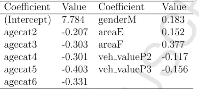
2.67GHz processors. After, the entropic betas are found by fitting a frequentist GLM with the posterior mean as response vector. Table 5 shows the entropic coefficients obtained for this example.

Coefficient

Value

Coefficient

Value

(Intercept) 7.784

genderM

0.183

agecat2

-0.207 areaE

0.152

agecat3

-0.303 areaF

0.377

agecat4

-0.301 veh valueP2 -0.117

agecat5

-0.403 veh valueP3 -0.156

agecat6

-0.331

Table 5: Entropic coefficients

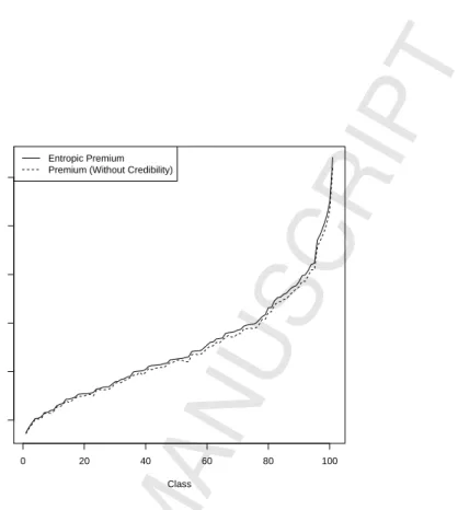
Corollary 5.1 can be used to obtain the entropic premium for each homogeneous class. We do not show here a full table of premium values since there are 101 classes and it would take too much space. Never-theless, a full table can be found at this article’s website in the section “Classes Table”. Figure 3 shows a graph of the entropic premiums in increasing order for all the classes in this example and compares it to premiums obtained using a frequentist GLM without any credibility considerations. We see that for some risk classes the GLM premiums are fully credible while for others the entropic credibility premiums are larger and more conservative.

Remark 6.1. The use of the uniform prior here is arbitrary and for illustrative purposes only. The goal here is not to seek the best Bayesian analysis to this particular dataset, but rather to illustrate the feasibility of our method. That is, to show that it can be used with real–life datasets and get the results in a reasonable amount of time. It is up to the user of the method to choose a prior based on the criterion of their preference.

Conclusion

As a Bayesian model, linear credibility (described at the beginning of the introduction) is rather artificial: the adequacy of Jewell’s prior in any given situation is never discussed and the main focus is to en-sure a credibility premium that is easy to compute. This convenience was crucial when B¨uhlman and Jewell originally published their work

0 20 40 60 80 100 1500 2000 2500 3000 3500 4000 Class Premium Entropic Premium Premium (Without Credibility)

Figure 3: Entropic credibility premiums in increasing

order

since computing power was scarce and expensive. Nowadays, not only computing power is cheap, but also sophisticated simulation software is available to anyone on the internet.

We propose then a modern Bayesian approach to credibility. In this way one can choose a prior based on out–of–sample information rather than on ease of computation. The limitation of possible priors is now set by the convergence of MCMC simulations. We use the relative entropy between the “true” model and the estimated one as the loss function.

Our proposal, when compared to classical credibility results for the exponential families, has the additional advantage of considering the uncertainty on the dispersion parameter. Finally, applying our method to a publicly available dataset shows that although substantial computations are required to obtain the credibility estimates, it is possible to apply this method to real–life datasets.

Acknowledgments

The authors are sincerely grateful to the anonymous reviewers for their constructive comments. We dedicate this paper to the memory of Bent Jørgensen whose contribution to the theory of exponential dispersion families opened the way for future developments.

References

[1] Jos´e M. Bernardo. Intrinsic credible regions: An objective bayesian approach to interval estimation. Test, 14(2):317–384, 2005.

[2] H. B¨uhlmann. Experience rating and credibility.ASTIN Bulletin, 4(3):99–207, 1967.

[3] H. E. Daniels. Exact saddlepoint approximations. Biometrika, 67(1):59–63, 1980. URLhttp://biomet.oxfordjournals.org/ content/67/1/59.abstract.

[4] P. de Jong and G.Z. Heller. Generalized Linear

Mod-els for Insurance Data. Cambridge University Press, 2008.

ISBN 9780511755408. URL http://dx.doi.org/10.1017/ CBO9780511755408. Cambridge Books Online.

[5] F.E. De Vylder. Non-linear regression in credibility theory.

Insurance: Mathematics and Economics, 4(3):163–172, 1985.

URLhttp://EconPapers.repec.org/RePEc:eee:insuma:v:4: y:1985:i:3:p:163-172.

[6] P. Diaconis and D. Ylvisaker. Conjugate priors for exponen-tial families. The Annals of Statistics, 7(2):269–281, 1979. URL

http://dx.doi.org/10.1214/aos/1176344611.

[7] C.A. Hachemeister. Credibility for regression models with appli-cation to trend. Proc. of the Berkeley Actuarial Research

Con-ference on Credibility, pages 129–163, 1975.

[8] W.S. Jewell. Credible means are exact Bayesian for exponential families. ASTIN Bulletin, 8(1):77–90, 1974.

[9] N.L. Johnson. Uniqueness of a result in the theory of accident proneness. Biometrika, 44:530–531, 1957.

[10] B. Jørgensen. The Theory of Exponential Dispersion Models and

Analysis of Deviance. Instituto de Matem´atica Pura e Aplicada,

(IMPA), Brazil, 1992.

[11] B. Jørgensen. The Theory of Dispersion Models. Chapman & Hall, London, 1997.

[12] R. Kaas, M Goovaerts, J Dhaene, and M. Denuit. Modern

Actu-arial Risk Theory. Springer-Verlag Berlin Heidelberg, 2008.

[13] S. Kullback. Information Theory and Statistics. Dover Publica-tions, New York, 1968.

[14] S. Kullback and R. A. Leibler. On information and sufficiency.

The Annals of Mathematical Statistics, 22(1):79–86, 1951. URL

http://dx.doi.org/10.1214/aoms/1177729694.

[15] Z.M. Landsman and U.E. Makov. Exponential dispersion mod-els and credibility. Scandinavian Actuarial Journal, 1998(1):89– 96, 1998. URL http://dx.doi.org/10.1080/03461238.1998. 10413995.

[16] J. A. Nelder and R. W. M. Wedderburn. Generalized linear

mod-els. Journal of the Royal Statistical Society, Series A, General,

135:370–384, 1972.

[17] J.A. Nelder and R.J. Verall. Credibility theory and generalized linear models. ASTIN Bulletin, 27(1):71–82, 1997.

[18] E. Ohlsson. Combining generalized linear models and credibility models in practice.Scandinavian Actuarial Journal, 2008(4):301– 314, 2008.

[19] R Core Team. R: A Language and Environment for Statistical

Computing. R Foundation for Statistical Computing, Vienna,

Austria, 2017. URLhttps://www.R-project.org/.

[20] Stan Development Team. RStan: the R interface to Stan, 2016. URLhttp://mc-stan.org/. R package version 2.14.1.

Appendix: Proofs of technical lemmas

Proof of Lemma 3.1

Let d be the unit deviance function of the response distribution and

y, µ_∈Ω. By (7), we have that

d(y, µ) = 2yκ˙−1(y)−κ˙−1(µ) −κ( ˙κ−1(y)) +κ( ˙κ−1(µ)) = 2yκ˙−1(y)−κ( ˙κ−1(y))+ 2κ( ˙κ−1(µ))−yκ˙−1(µ)

=d1(y) +d2(y, µ),

whered1(y) = 2yκ˙−1(y)−κ( ˙κ−1(y))andd2(y, µ) = 2κ( ˙κ−1(µ))−yκ˙−1(µ).

Now, letY be a random variable with support in Ω andµ_∈Ω be fixed, then E[d2(Y, µ)] =E2κ( ˙κ−1(µ))−Yκ˙−1(µ) = 2κ( ˙κ−1(µ))₋E[Y] ˙κ−1(µ) =d2(E[Y], µ). Proof of Lemma 3.2

The first part is a direct consequence of (17). Since y is fixed, mini-mizing the right hand side is equivalent to minimini-mizingd2and therefore

the claim is true.

The unit deviance dis such that (see Chapter 1 of Jørgensen [11])

d(y, µ) > 0 if y ₆= µ and d(y, µ) = 0 when y = µ. Thus d(y, µ) is minimized when y = µ and by Part 1 above the same applies to

d2(y, µ).

Proof of Lemma 5.1

From the definition of Dand Lemma 3.1, we have that

D(y,µ) = m X i=1 wid(yi, µi) = m X i=1 wi(d1(yi) +d2(yi, µi)) = m X i=1 wid1(yi) + m X i=1 wid2(yi, µi) =D1(y) +D2(y,µ),

whereD1(y) =Pmi=1wid1(yi) andD2(y,µ) =Pmi=1wid2(yi, µi). This

proves (22). Let Y = (Y1, . . . , Ym) be a random vector with support

on Ωm, andµ_∈Ωmbe fixed. Then

E[D2(Y,µ)] =E[ m X i=1 wid2(Yi, µi)] = m X i=1 wid2(E[Yi], µi) =D2(E[Y],µ), which proves (23).