Multi-objective worst case optimization by means of evolutionary algorithms

http://go.warwick.ac.uk/lib-publications

Original citation:

Branke, Juergen, Avigad, Gideon and Moshaiov, Amiram (2013) Multi-objective worst

case optimization by means of evolutionary algorithms. Working Paper. Coventry, UK:

WBS, University of Warwick. (WBS working papers)

Permanent WRAP url:

http://wrap.warwick.ac.uk/55724

Copyright and reuse:

The Warwick Research Archive Portal (WRAP) makes this work of researchers of the

University of Warwick available open access under the following conditions. Copyright ©

and all moral rights to the version of the paper presented here belong to the individual

author(s) and/or other copyright owners. To the extent reasonable and practicable the

material made available in WRAP has been checked for eligibility before being made

available.

Copies of full items can be used for personal research or study, educational, or

not-for-profit purposes without prior permission or charge. Provided that the authors, title and

full bibliographic details are credited, a hyperlink and/or URL is given for the original

metadata page and the content is not changed in any way.

A note on versions:

The version presented here is a working paper or pre-print that may be later published

elsewhere. If a published version is known of, the above WRAP url will contain details

on finding it.

by Means of Evolutionary Algorithms

J ¨urgen Branke

University of Warwick, UK

Gideon Avigad

Braude College of Engineering, Israel

Amiram Moshaiov

Tel Aviv University, Israel

Abstract

Many real-world optimization problems are subject to uncertainty. A possible goal is then to find a solution which is robust in the sense that it has the best worst-case performance over all possible scenarios. However, if the problem also involves mul-tiple objectives, which scenario is “best” or “worst” depends on the user’s weighting of the different criteria, which is generally difficult to specify before alternatives are known. Evolutionary multi-objective optimization avoids this problem by searching for the whole front of Pareto optimal solutions. This paper extends the concept of Pareto dominance to worst case optimization problems and demonstrates how evolu-tionary algorithms can be used for worst case optimization in a multi-objective setting.

Keywords

Worst-case optimization, robustness, multi-objective evolutionary algorithm, uncer-tainty.

1

Introduction

Many practical real-world optimization problems require dealing with uncertainty, e.g., because they rely on forecasts, because they depend on an opponent’s move, because of delayed decisions in hierarchical planning, or because the solution eventually im-plemented is subject to manufacturing tolerances. In such cases, one typically searches forrobustsolutions. What exactly constitutes a robust solution depends on the specific application and user needs, but often used criteria are a goodexpectedquality, a low variance or good performance in the worst case. In this paper, we assume that a solu-tion’s quality depends on a number of possible scenarios, and the solution is considered robust if it performs well in theworstcase. Considering the worst case is important in particular if the decision maker is very risk averse, or if the stakes are high, such as in situations involving potential bankruptcy or death.

Another common characteristic of real-world problems is that they involve mul-tiple objectives which need to be considered simultaneously. As these objectives are usually conflicting, it is not possible to find a single solution that is optimal with re-spect to all objectives. Which solution is the best depends on the user’s utility function, i.e., on how the different criteria are weighted. Unfortunately, it is usually rather diffi-cult to formally specify user preferences before the alternatives are known. One way to solve this predicament is by searching for the whole Pareto-optimal front of solutions,

i.e., all solutions that can not be improved in any criterion without at least sacrificing another criterion. This set of solutions with different trade-offs between the objectives can then be inspected by a decision maker who selects the final solution. One particular approach to multi-objective optimization that has become quite popular in recent years is evolutionary multi-objective optimization (see, e.g., Deb, 2001). Because Evolution-ary algorithms (EAs) work with a population of solutions throughout the run, they are able to search for several Pareto-optimal solutions with different trade-offs simultane-ously in one optimization run.

In this paper, we extend the concept of Pareto dominance to worst case optimiza-tion. Furthermore, we show how the new concept can be integrated into EAs to allow them to search for worst case robust alternatives in a multi-objective setting. Note that in the case of multiple objectives, different decision makes may consider different sce-narios as worst-case. Thus, the problem requires special attention, as it is not possible to reduce a soltuionto a single point in the objective space (as done, e.g., for MO robust-ness optimization).

The paper is structured as follows. Section 2 briefly surveys related work and briefly introduces evolutionary multi-objective optimization. Our extensions to worst case multi-objective optimization are presented in Section 3. Two suggested alterna-tives are then compared in Section 4. The paper concludes with a summary and some ideas for future work.

2

Fundamentals and related work

In the past decade, there has been a tremendous interest in evolutionary multi-objective optimization, and the on-line repository (emo) currently lists more than 2600 papers in this area. A main cause for this interest is certainly the EA’s capability to work with a population of solutions, and thus to generate, in one run, a set of alternatives with different trade-offs between the objectives, which can then be presented to a decision maker to choose from.

A comprehensive introduction to the field of multi-objective evolutionary algo-rithms (MOEAs) is out of the scope of this paper, and the interested reader is referred to e.g. Deb (2001); Coello Coello et al. (2002). In the following, we will focus on the aspects particularly relevant for our approach.

Usually, the comparison of solutions in the case of multiple objectives is based on the concept of dominance. A solutionxis said to dominate a solutionyif and only if solutionxis at least as good asyin all objectives, and strictly better in at least one ob-jective. More formally, for a minimization problem (which we will assume throughout the paper without loss of generality), dominance can be specified as follows:

xy ⇔ ∀i∈[1. . . m] :fi(x)≤fi(y)

∧∃j∈[1. . . m] :fj(x)< fj(y)

Figure 1 illustrates the concept for the case of two objectives. In that example, so-lution C is dominated by soso-lution A and B, while soso-lutions A and B are non-dominated and thus, without any additional information about the DM’s preferences, have to be considered incommensurable. If a solution is non-dominated with respect to any other solution in the search space it is called Pareto-optimal.

C B A area dominated X by solution X Legend: f = criterion 1 f = criterion 22 1

Figure 1: Illustration of the standard dominance relation

Pareto-optimal front, and second, it has to maintain diversity along this front. There are several successful MOEA variants, including SPEA-2 Zitzler et al. (2002) and NSGA-II Deb (2001).

2.2 Evolutionary search for robust solutions

In recent years, there has been a growing interest in applying evolutionary computa-tion to optimizacomputa-tion problems involving uncertainty, and a recent survey on this field can be found in Jin and Branke (2005). One typical goal in many real world optimiza-tion scenarios involving uncertainty is to produce soluoptimiza-tions that are not only of high quality, but also robust. There are many possible notions of robustness, including a good expected performance, a good worst-case performance, a low variability in per-formance, or a large range of disturbances still leading to acceptable performance (see also Branke, 2001b, p. 127). Yet another definition would be a solution’s probability to violate the constraints, which is often calledreliability.

There are at least four different possibilities to integrate the notion of robust-ness/reliability into evolutionary algorithms:

1. Simply optimize a robustness measure such as the expected performance, or the worst-case performance.

2. Penalize solutions that are not robust, e.g., solutions with high variance.

3. Put a constraint on the robustness of a solution, i.e., only accept solutions with a minimal robustness.

4. Consider robustness as an additional objective and use an MOEA to generate dif-ferent possible trade-offs.

Most research work on evolutionary robustness optimization today attempts to optimize theexpectedfitness given a probability distribution of the uncertain variable. From the point of view of the optimization approach, this reduces the fitness distribu-tion to a single value, theexpectedfitness. Thus, in principle, standard evolutionary algorithms could be used. Unfortunately, it is usually not possible tocalculatethe ex-pected fitness analytically, it has to beestimated. This, in turn, raises the question how to estimate the expected fitness efficiently, and how to optimize based on estimates.

1. Implicit averaging:Tsutsui and Ghosh (1997) have shown that a genetic algorithm with infinite population size and very rough estimates of the fitness (a single sam-ple from the stochastic evaluation function) behaves, on average, exactly as a ge-netic algorithm working on the expected fitness. Intuitively, this can be explained by the fact that an EA generates many similar solutions in promising areas of the search space, and thus the over-evaluation of one particular solution is counter-balanced by the under-evaluation of a similar solution. This feature is sometimes termed “implicit averaging”.

2. Explicit averaging over multiple samples:Averaging overnsamples reduces the standard deviation of the estimator by a factor of√n, while it increases the com-putational cost by a factor ofn, which makes this method often impractical. Nev-ertheless, it is used frequently, see e.g. Greiner (1996); Sebald and Fogel (1992); Thompson (1998); Wiesmann et al. (1998).

3. Variance reduction techniques: Using derandomized sampling techniques in-stead of random sampling reduces the variance of the estimator, thus allowing a more accurate estimate with fewer samples. In Loughlin and Ranjithan (1999); Branke (2001b),Latin Hypercube Samplingis employed, together with the idea to use the same disturbances for all individuals in a generation.

4. Evaluating important individuals more often: In Branke (1998), it is suggested to evaluate good individuals more often than bad ones, because good individu-als are more likely to survive and therefore a more accurate estimate is benefi-cial. In Branke (2001a), it was proposed that individuals with high fitness variance should be evaluated more often. Stagge (1998) considered a(µ, λ)or(µ+λ) evo-lution strategy and suggested that the sample size should be based on an individ-ual’s probability to be among theµbest ones. More elaborate strategies to decide which individual to evaluate how often have been proposed in in Buchholz and Th ¨ummler (2005) and Schmidt et al. (2006).

5. Using other individuals in the neighborhood: Since promising regions in the search space are sampled several times, it is possible to use information about other individuals in the neighborhood to estimate an individual’s expected fitness. In particular, in Branke (1998) it is proposed to record thehistoryof an evolution, i.e. to accumulate all individuals of an evolutionary run with corresponding fit-ness values in a database, and to use the weighted average fitfit-ness of neighboring history individuals. More elaborate schemes involving the use of local approxima-tion models can be found in Paenke et al. (2006); Sano and Kita (2000).

Robustness based on expected fitness has also been studied for the case of mul-tiobjective problems (Deb and Gupta, 2005; Gupta and Deb, 2005;?). Two notions of robustness are studied, one optimizing the mean objective values, the other optimizing under the constraint that the distance between mean and undisturbed fitness is less than some threshold. In both cases, sampling is used for estimation. Then, a standard MOEA is used to work with these expected fitnesses and/or the estimated constraint violation. Gupta and Deb (2005) thereby extends Deb and Gupta (2005) by additionally taking into account robustness with respect to constraint violations. ?summarizes the former two and examines the issues in more detail.

In contrast to the expected fitness approach, theworst casecan usually not be ob-tained by sampling. Instead, finding the worst case for a particular solution may itself

be a complex optimization problem. In Elishakoff et al. (1994), this is solved by run-ning an embedded optimizer searching for the worst case for each individual (called anti-optimization in Elishakoff et al. (1994)). Similarly, Ong et al. (2006) construct a sim-plified meta-model around a solution, and use a simple embedded local hill-climber to search for the worst case. Lim et al. (2006) use the maximum disturbance range that guarantees fitness above a certain threshold. Again, this is determined by an embed-ded search algorithm. Tjornfelt-Jensen and Hansen (1999) uses a coevolutionary ap-proach for a scheduling problem, co-evolving solutions and worst-case disturbances. Others simply calculate some bounds on the worst-case behavior (e.g., Pantelides and Ganzerli (1998)). Lua et al. (2005) use worst-case performance in the case of a multi objective problem, but they assume that the user provides some a priori knowledge in the form of a target point, and then evaluate individuals with respect to the scenario which leads to the largest distance from the target as worst case. This in effect reduces the multi-objective problem to a single objective (distance from target) problem.

A few papers treat robustness as an additional criterion to be optimized. Robust-ness is measured, e.g., as variance (Das, 2000; Jin and Sendhoff, 2003; Paenke et al., 2006), as maximal range in parameter variation that still leads to an acceptable solu-tion (Li et al., 2005; Lim et al., 2006), or as the probability to violate a constraint (Deb et al., 2007; Daum et al., 2007). This allows the decision maker to analyze the possi-ble trade-off between solution quality and robustness/reliability. The challenges and approaches are mainly similar to the single objective optimization in determining the performance measures.

Our paper extends the notion of worst-case robustness optimization to the multi-objective case. That is, for an inherently multi-multi-objective problem and a user interested in the worst case, we want to generate a set of solutions with different trade-offs to choose from. In some sense, this is similar to the multi-objective problems considered by Gupta and Deb (2005), but instead of looking at the expected fitness, we look at worst-case fitness. While in a single objective setting, it makes little difference whether expected fitness or worst-case fitness is optimized, there is a huge difference in a multi-objective setting. The reason is that in the case of multiple multi-objectives, different users may consider different scenarios as worst case, and thus it is no longer possible to reduce a solution to a single point in the objective space.

To our best knowledge, the first attempt to handle worst-case robustness in a Pareto sense may be attributed to Avigad et al. (2005). They have considered it for the problem of robust conceptual design as related to the issue of delayed decisions. How-ever, the focus of the current paper is much broader, with a completely new algorithm to handle worst-case dominance relations.

3

Selection in multi-objective worst-case optimization

In ordinary multi-objective optimization, a solutionxis represented by a single point in objective space, i.e. by a vector of fitness valuesf~(x). For worst-case optimization, a solution’s fitness vector is not fully determined, but depends on some external, uncon-trollable parameters. In other words, in objective space, a solution is now represented by a set of fitness vectors,F = {f~(1)_{(x), ~f}(2)_{(x), ~f}(3)_{(x), . . .}. In principle, the set F}

could be infinite, although we focus here on settings where the uncertainty can be cap-tured by a finite set of scenarios.

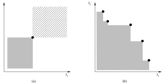
f₂ f₁ (1) (2) (3) (4) (5) (6) (7) (8)

Figure 2: Set of representativesF of a solution. The representative labeled (8) is the worst-case representative for a user only caring about objectivef1, the solution labeled

(5) is the worst-case representative for a user weighting both objectives equally. The line connects all potential worst-case representatives(W).

search towards the Pareto optimal front, while at the same time maintaining diversity of non-dominated solutions. For example in NSGA-II, an individual’s fitness is calcu-lated based on two mechanisms: the non-dominance sorting, and the crowding dis-tance calculation. The idea of the non-dominance sorting is to favor individuals close to the non-dominated front. It recursively looks at all the individuals in the population, determines the subset of non-dominated individuals, assigns them the next best rank, and removes them from the population, until all individuals have been ranked. To war-rant diversity in the population, individuals with the same non-domination rank are sorted with respect to their crowding distance, which is the sum of distances between their closest left and right neighbor, over all dimensions. Amongst individuals with the same non-domination rank, those with a larger crowding distance are preferred.

For multi-objective worst-case optimization, these ideas can not be applied directly because the concept of non-dominance has not yet been defined for worst-case opti-mization, and because each individual is represented by a set of fitness vectors, which makes it impossible to calculate a crowding distance.

Figure 2 illustrates the set of fitness vectorsFrepresenting a particular solution. In this example,F consists of eight discrete points in the 2-dimensional objective space. Depending on the user’s preferences different representatives constitute the worst case. For example, for a user only interested in minimizing objectivef1, the representative

labeled (8) would be considered worst case, while for a user with equal weighting for both objectives, the solution labeled (5) would be considered worst case. But no mat-ter how the user’s utility function, of the eight representatives, only those connected by the dotted line could ever be worst-case representatives. Therefore, the three other representatives can be ignored for multi-objective worst-case optimization. We denote the set of possible worst-case representatives byW. Note that the worst-case represen-tatives are just the set of non-dominated solutions for theinvertedMO problem with

f₂ f₁ (a) f₂ f₁ (b)

Figure 3: Visualization of the concept of dominance for ordinary MO optimization (left) and MO worst-case optimization (right).

maximizationof all objectives.

In the following, we assume that we can somehow determineW, e.g., because the set of considered scenarios is known and finite. In some cases, determiningWmay not be trivial but if necessary, could also be determined by running an embedded MOEA on the inverted problem.

3.2 Worst-case dominance relation

In this subsection, we examine the implications of the worst-case condition on domi-nance relationships. Figure 3 compares the areas dominated in ordinary MO optimiza-tion and MO worst-case optimizaoptimiza-tion. In the ordinary case (left panel), a soluoptimiza-tionx

dominates all solutions that are worse in both objectives, which is the striped area to the upper right. Similarly, it is dominated by all solutions in the grey area. If another solutionyis in none of the two above areas, it depends on the user’s preferences which solution is considered better, and the solutions are said to be non-dominated. For MO worst-case optimization (right panel), we have to deal with sets of worst-case represen-tativesW(x)(one for each solution). A natural definition of dominance in the case of worst-case multi-objective optimization would be:

Definition: Solution xworst-case dominates solutiony (denoted asy wc x), if

there exists no utility function such that a user would preferywith respect to the worst-case scenarios for this user.

Since this definition depends on the worst-case representatives of both solutions

W(x)andW(y), it is not possible to specify in general an area dominated byx. How-ever, we can specify that for a solution y with W(y) completely within the domi-nated region ofW(x)for the inverted (maximization) problem (the grey area in Fig-ure 3, right panel),yworst-case dominatesx, because no member ofW(y)could ever be considered worst case relative to the members in W(x). Thus, in order to deter-mine whether one solution worst-case dominates another, we can deterdeter-mine the non-dominated representatives ofW(x)∪ W(y)with respect to the inverted problem. If all

f₂ f₁ (a) f₂ f₁ (b)

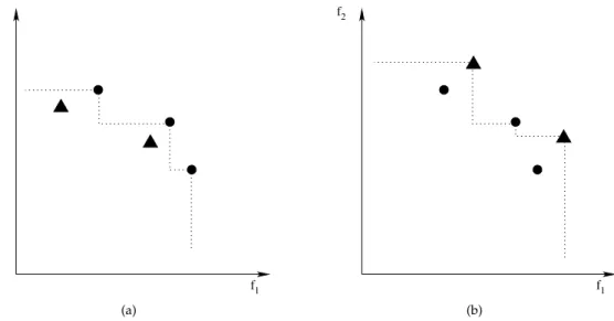
Figure 4: Example for one solution represented by triangles dominating the other (left), and two non-dominated solutions (right). The line indicates the non-dominated front for the inverted problem.

non-dominated representatives belong toW(x), then solutionyworst-case dominates

x(denoted asy wc x). If all non-dominated representatives belong toW(y), then

so-lutionxworst-case dominatesy(xwc y). Otherwise, the two solutions are worst-case

non-dominated.

Two examples are provided in Figure 4. In the left panel, the non-dominated repre-sentatives of the inverted problem all belong to the solution drawn with bullets, i.e., it is worst-case dominated by the triangle-solution. In the right panel, some non-dominated representatives of the inverted problem belong to either solution, i.e., the two solutions are worst-case non-dominated.

The concept of non-dominance can be extended to more than two solutions: Lemma: A solutiony is worst-case non-dominated with respect to a set of solu-tionsx1, . . . , xnif and only ifyis worst-case non-dominated with respect to each of the

solutionsx1, . . . , xnindividually.

Proof: If y is worst-case non-dominated with respect to each of the solutions

x1, . . . , xnindividually, then there is at least one possible utility function whereywould

be the worst-case preferred solution and thus non-dominated. This utility function would equally value the border of the dominated area of the inverted problem of all representatives ofy. All representatives of the other solutions necessarily lie outside of the dominated area and are thus less valued by any decision maker. The opposite direction is trivial.2

The above worst-case dominance relation can be used to construct a worst-case dominance ranking similar to what is used in NSGA-II. First, all solutions non-dominated with respect to all other solutions are identified and assigned Rank 1. Then they are removed from the population, and the non-dominated solutions of the remain-ing individuals are identified and assigned Rank 2, etc.

5 6 7 8 9 10 0 1 2 3 4 5 6 7 objective 2 objective 1 (a) Diversity preservation

0 1 2 3 4 5 6 7 8 0 1 2 3 4 5 6 7 8 objective 2 objective 1 (b) Small spread 6 7 8 1 2 3 4 5 objective 2 objective 1 (c) Convexity

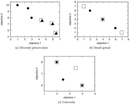
Figure 5: When comparing mutually non-dominating solutions, different criteria may play a role. In all three examples, the solution represented by bullets should be pre-ferred over the solution represented by squares. In (a), it better preserves diversity; in (b), it has a lower spread, and in (c), the representatives define a convex rather than concave region.

3.3 Ranking individuals within a front

Having established a means to determine whether one solution dominates another one, we can now use non-dominated sorting as in NSGA-II to rank the solutions, only using our newly proposed concept of worst-case dominancy instead of the usual dominance concept. The next step is to ensure diversity among solutions by preferring those solu-tions that are in less crowded regions.

As has been noted above, in standard NSGA-II, individuals of the same non-dominated rank are compared based on crowding distance, which is not defined for our application, because each solution consists of a set of representatives in objective space. Also, while diversity is probably still important, it is not the only criterion. For example, the spread of a solution’s representatives is an additional criterion. It repre-sents the uncertainty involved in a decision and should be minimized. Also, a convex set should be preferred to a concave set. The three criteria diversity, spread, and con-vexity are visualized in Figure 5.

In the following two subsections, we present two alternatives to compare indi-viduals within a non-domination front which should implicitly take into account the

aforementioned criteria diversity, spread, and convexity. Note that they are used only for individuals with the same non-dominated rank, and that the extreme individuals (best if only objectivefiis considered) always receive the best fitness within a rank in

our implementation.

3.3.1 Expected marginal utility

The first approach uses the utility-based crowding as suggested in Branke et al. (2004). The underlying idea is that each decision maker (DM) has an underlying utility func-tion used to pick the final solufunc-tion. Given a space and probability distribufunc-tion of utility functions, it is possible to estimate each solution’sexpected marginalutility, which is de-fined as the expected loss a DM would suffer if this solution were removed from the set. Then, among solutions in the same Pareto rank, those with a higher expected marginal utility are favored.

In principle, arbitrary utility function and distributions could be used. In the ex-amples below, we restrict ourselves to two objectives, a linear utility functions of the form

U(x, λ) =−λf1(x) + (λ−1)f2(x) (1)

and a uniform probability forλ ∈ [0,1]. This utility function is easily adapted to the case of worst-case utility simply by taking the minimum over all representatives. That is, withmrepresentativesx(1)_{, . . . , x}(m)_{utility is calculated as}

U(x, λ) = min

j=1...m{−λf1(x

(j)_{) + (λ−1)f}

2(x(j))}. (2)

Based on the utility, the marginal utility of a particular solutionxi_,U0_(xi_{), can be}

defined as

U0(xi, λ) = max{0,min

j6=i{U(x

i_{, λ)−U(x}j_{, λ)}}}

and the expected marginal utility given a probability distributionP(λ)is then

E(U0(x)) = Z

λ

U0(x, λ)·P(λ)dλ

The expected marginal utility can be estimated by Monte-Carlo integration over all λ. In the examples below, We estimate the expected marginal utility by generat-ingk randomλby stratified sampling (i.e. one randomλfrom each of the intervals

[0,1/k[; [1/k,2/k[;. . .; [k−1/k,1]). For each solution, the marginal utilities for allλare computed and summed up. Note that in our worst-case scenario, a solution’s utility for a specificλis the minimal utility over all the solution’s representatives.

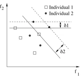
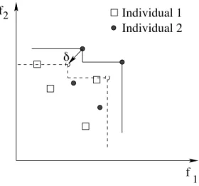
The marginal utility for two possible utility functions is visualized in Figure 6. 3.3.2 δ+_-indicator

The second criterion we propose involves the distance a set of worst-case representa-tives can be moved until the solution becomes dominated, or have to be moved until it is non-dominated. It is closely related to the binary additive-indicator proposed by Zitzler et al. (2003), so we start by discussing this first.

The binary additive -indicatorI+ of two Pareto set approximations1 is equal to the minimum distance by which a Pareto set approximation needs to or can be

Individual 1

Individual 2

f

f

2

1

Figure 6: If the solution represented by squares would be removed, the user only inter-ested in minimizing objectivef2would suffer a loss ofδ1, while a user equally

weight-ing the two objectives would suffer a loss ofδ2.

translated in each dimension in the objective space such that another approximation is weakly dominated. Formally, it is defined as follows for two approximation setsA

andB:

I+(A, B) = min

{∀x∈B∃y∈A:fi(y)−≤fi(x)fori∈ {1, . . . , n}} (3)

The general idea of the+_{indicator can be adapted to the case of worst-case}

dom-inancy. For distinction, we call the resultδ+ _{indicator. Again, the intuitive meaning}

ofδ+_{(A, B)is by how much one has to translateAin each dimension of the objective}

space such that it dominatesB, but with domination now being calculated according to the worst-case domination criterion:

Iδ+(W1,W2) = min

{∀x∈ W1∃y∈ W2:fi(y)≥fi(x)−fori∈ {1, . . . , n}} (4)

In practice, this can be computed as

Iδ+(W1,W2) = max x∈W1 min y∈W2 max 1≤i≤nfi(x)−fi(y) (5)

The δ+ indicator allows us to compare two sets of worst-case representatives. However, for selection, we need to define how good a solution is with respect to all others. In the indicator-based MOEA proposed in Zitzler and K ¨unzli (2004), this is achieved, e.g., by using a weighted sum of the epsilon-indicator of a solution in com-parison to all other solutions. However, this involves additional parameters and re-quires proper scaling. Therefore, we propose here to define a solution’s surrogate fitness F(x) as the minimum distance a solution has to be moved to become non-dominated, or, if it is already non-non-dominated, the maximum distance it can be moved until it becomes dominated. Formally, this can be expressed as

F(x) = min

y∈P\x

Individual 1

Individual 2

f

f

Figure 7: In this example, the solution represented by squares dominates the solution represented by bullets. For the bullets to become non-dominated, they would have to be shifted by at leastδin both objectives.

wherePis the population of all individuals. An example is provided in Figure 7. Furthermore, we assign the best solutions in either objective very high values to keep them in the population.

4

Comparison of expected marginal utility and

δ

measures

In this section, we will compare the two proposed measures to distinguish individuals which are in the same non-dominated front, namely the marginal utility approach and theδ+_approach.

First, in the next subsection, we compare the two approaches based on some partic-ular examples to understand how they reflect the criteria diversity, spread, and convex-ity introduced above. Following this comparison, we present some empirical results a simple artificial test functions.

4.1 Diversity, spread, convexity

To see how the two approaches handle diversity, spread, and convexity, we have taken the three examples from Figure 5 and report on the fitness values determined by all three methods.

Regarding diversity, the fitness values computed by the two approaches for each of the three solutions from Figure 5(a) are reported in Table 1. As can be seen, both approaches rank the isolated solution represented by bullets as best. The other two are valued equally by theδ+measure, as the distance they need to be shifted is equal in both cases. For the marginal utility measure, the square solution has a fitness of 0, as it is never optimal for a linear utility function, and the solution represented by triangles scores second best. Thus, at least for this particular example, the marginal utility approach better captures the diversity criterion.

For the convexity criterion (Figure 5 (c)), both approaches assign a fitness of 0 to the individuals represented by squares (because it is never better than the other indi-vidual, or because a minimal shift would make it dominated), and a fitness of 1.0 to the individual represented by bullets.

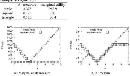
Table 1: Fitness values computed by marginal utility approach andδ+_{measure for the}

example of Figure 5 (a).

δ+_{measure marginal utility}

circle 3.375 987.9 square 0.125 0.0 triangle 0.125 30.4 0 200 400 600 800 1000 1200 1400 1600 1800 2000 0 1 2 3 4 5 6 Fitness circle fixed square varied

(a) Marginal utility measure

0 0.5 1 1.5 2 2.5 3 3.5 4 0 1 2 3 4 5 6 Fitness circle fixed square varied (b)δ+_measure

Figure 8: Fitness of the two individuals represented by bullets and squares in Figure 5 (b), where the spread of the square solution is varied. Left panel (a) shows fitness measured as marginal utility, while right panel shows fitness measured according to

δ+measure.

Finally, for the spread criterion, we look at how the fitness changes depending on the distance between the representatives. To this end, we fix the locations of all rep-resentatives of the solution represented by squares. For the solution represented by bullets, we place the representatives at the coordinates(4,4)(same center representa-tive as other solution),(4−∆,4 + ∆), and(4 + ∆,4−∆). For∆ = 2, the two solutions are identical, while for∆ <2, the circle solution has a smaller spread, and for∆ >2, it has a larger spread. Figure 8 compares the fitness of both solutions depending on∆, for both approaches.

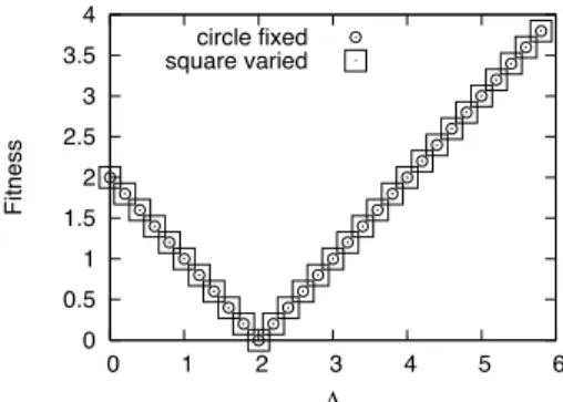
The plot for the utility measure (Figure 8 (a)) shows the intuitively expected be-havior: Always the solution with the smaller spread is preferred. For theδ+measure, this is only true for∆<1and∆>2. Within this range, the two solutions are consid-ered equivalent. Results are even more surprising if the middle representative of both solutions is removed, see Figure 9. In this case, theδ+ measure computes the same fitness for both individuals, independent of∆. On the other hand, the utility measure is not affected by the presence or absence of the middle representative, as this is never the worst representative in the case of linear utility functions.

Overall, the above examples seem to suggest that the utility measure is closer to what one would intuitively regard as a good measure.

4.2 Empirical comparison

Instead of looking at some particular combinations of individuals, in this subsection, we want to compare the two approaches empirically on a simple, artificial test prob-lem. We don’t want to impose additional difficulties by using a difficult optimization

0 0.5 1 1.5 2 2.5 3 3.5 4 0 1 2 3 4 5 6 Fitness circle fixed square varied

Figure 9: Same plot as in Figure 8 (b), but with middle representative removed.

-0.2 0 0.2 0.4 0.6 0.8 1 1.2 -0.2 0 0.2 0.4 0.6 0.8 1 1.2

Figure 10: Worst-case representatives for some exemplary solutions of the suggested test problem.

problem, but simply want to see whether the resulting distribution of individuals along the Pareto front is good with respect to a worst-case optimization. Thus, we here use a very simple test problem, the 10-dimensional ZDT1, from which we artificially create scenarios. For each solution which would usually have the objective valuesf1andf2,

we now create three representatives as follows. First, we calculate a disturbance fac-tord= 0.2exp(−f1(x)), i.e., the disturbance is larger for smaller values off1(x). The first two representatives are simply created by setting f₁(1)(x) = f1(x) +d, f

(1) 2 (x) =

f2(x)−d, f₁(2)(x) = f1(x)−d, f₂(2)(x) = f2(x) +d, i.e., with equal distance from the original position to the upper left and lower right. The midpoint is chosen depend-ing on the difference f1(x)−f2(x): d2 = max{−0.9,min{0.9, f1(x)−f2(x)}}, and

f₁(3)(x) = f1(x)−0.5d2, f (3)

2 (x) =f1(x) +d2. In other words, the fitnesses of the third

scenario correspond to the original fitnesses forf1(x) =f2(x), but is moved to the up-per right forf1(x)< f2(x)and to the lower left forf1(x)> f2(x). Overall, this artificial problem thus has solutions where the scenarios have different spread and some form a convex, some a concave front. Figure 10 shows some solutions by their corresponding worst-case representatives.

Except for the diversity measure, the EMO algorithm was more or less a standard NSGA-II with Gaussian mutation with mutation probabilitypm = 0.04and step size

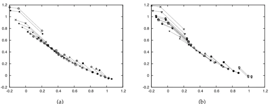
-0.2 0 0.2 0.4 0.6 0.8 1 1.2 -0.2 0 0.2 0.4 0.6 0.8 1 1.2 (a) -0.2 0 0.2 0.4 0.6 0.8 1 1.2 -0.2 0 0.2 0.4 0.6 0.8 1 1.2 (b)

Figure 11: Worst-case representatives for the final solutions obtained with a run using theδ+measure (left), and a run using the marginal utility measure (right).

population size makes the differences between the approaches more apparent. The algorithm was allowed to run for 200 generations. All results reported are averages over 100 runs.

Besides comparing the two approaches suggested in this paper, we also present results on a naive approach which reduces the three scenarios to one by averaging over all three scenarios. Removing the uncertainty by averaging is a simple yet common approach, and shall serve as a benchmark here.

An exemplary final population of theδ+measure and the marginal utility measure can be seen in Figure 11. Although population size is 20 and we have only 3 scenarios, such plots are relatively difficult to read, and it is hard to tell what approach performs better.

Therefore, we look at two performance measures:

1. The expected utility measured asλf1+ (1−λ)f2forλuniformly distributed in [0,1].

2. TheC(A, B)measure Zitzler et al. (2000). To compute this metric, we have com-bined the final populations of all 100 runs for each approach, and determined how many solutions from approach A are dominated by any solution from approach B

(C(A, B))and vice versa.

The expected utility, and its development over the 200 generations, can be seen in Figure 12. The methods proposed in this paper are both significantly better than the simple approach of removing the uncertainty by averaging (the standard error in the figure is too small to plot). The difference between marginal utility andδ+_measure

could also be attributed to the fact that we use expected utility as performance measure, which corresponds to the assumptions used for the marginal utility method.

The results for theC(A, B)measure are summarized in Table 2. As can be seen, almost all of the solutions generated by the averaging method are dominated by some solution found by the other approaches, while only very few solutions found by the utility approach or theδ+_{-measure approach are dominated by a solution found with}

the averaging method. This confirms the previous observation that the newly proposed approaches significantly outperform the method that simply averages over all scenar-ios. Comparing the utility measure and theδ+_{-measure, there seems to be a slight}

15 20 25 30 35 40 45 50 55 60 0 50 100 150 200 Expected utility Generation measure marginal utility averaging

Figure 12: Expected utility over the course of the run.

Table 2: C-measure comparisons of the different runs, comparing how many solutions of one run are worst-case-dominated by solutions of another. A: averaging, B: utility, C:δ+_-dominance by A B C A - 99.0 99.7 % dominated B 22.7 - 89.1 C 11.5 64.0

-advantage for theδ+_{-measure, but results are much less clear.}

5

Conclusion

In this paper, we have looked at worst-case multi-objective optimization, where a so-lution is evaluated by means of a finite set of different scenarios. As usual in multi-objective evolutionary optimization, the goal was to identify a good representative sub-set of solutions which is then presented to the decision maker to choose from. To our knowledge, this is the first attempt to transfer multi-objective evolutionary algorithms to worst-case optimization, without removing the multi-objectivity of the problem. The particular challenge is that it is not possible to reduce a solution to a single worst-case representative, because different users would consider different representatives as their worst case.

For this reason, we had to extended the definition of dominance for worst-case optimization on sets of representatives, which allowed us to perform non-dominated ranking of the solutions. For distinguishing between solutions of the same non-domination rank, we adapted two measures, one based on expected marginal util-ity, the other based on the distance a solution needs to be shifted to become (non-)dominated.

We compared the two measures on a few specific examples and a simple artificial test problems. The expected marginal utility measure seems to adhere better to the

intuition about what kind of solutions should be preferable. Both measures work sig-nificantly better than the simple idea of just ignoring the uncertainty and working with the expected (mean) objective values.

So far, the approach has been tested only on problems with two objectives, but an extension to more objectives should be straightforward. During the empirical analysis, it also became apparent that simply visualizing the resulting set of solutions (as is often done for MOEAs) is not very helpful. Better user interfaces, allowing to navigate along the Pareto front, would be needed for worst case multi-objective optimization. Finally, we plan to extend the approach from a finite set of scenarios to arbitrary worst-case multi-objective optimization problems, where an “embedded” EA is used to determine the worst-case front of a particular solution.

References

Avigad, G., A. Moshaiov, and N. Brauner (2005). MOEA-based approach to delayed decisions for robust conceptual design. InApplications of Evolutionary Computing, Volume 3449 ofLNCS, pp. 584 – 589. Springer. Branke, J. (1998). Creating robust solutions by means of an evolutionary algorithm. In A. E. Eiben, T. B¨ack, M. Schoenauer, and H.-P. Schwefel (Eds.),Parallel Problem Solving from Nature, Volume 1498 ofLNCS, pp. 119–128. Springer.

Branke, J. (2001a).Evolutionary Optimization in Dynamic Environments. Kluwer.

Branke, J. (2001b). Reducing the sampling variance when searching for robust solutions. In L. S. et al. (Ed.), Genetic and Evolutionary Computation Conference (GECCO’01), pp. 235–242. Morgan Kaufmann.

Branke, J., K. Deb, H. Dierolf, and M. Osswald (2004). Finding knees in multi-objective optimization. In Parallel Problem Solving from Nature, Number 3242 in LNCS, pp. 722–731. Springer.

Buchholz, P. and A. Th ¨ummler (2005). Enhancing evolutionary algorithms with statistical selection proce-dures for simulation optimization. In M. E. Kuhl et al. (Eds.),Winter Simulation Conference, pp. 842–852. IEEE.

Coello Coello, C. A., D. A. V. Veldhuizen, and G. B. Lamont (2002).Evolutionary Algorithms for Solving Multi-Objective Problems. Kluwer.

Das, I. (2000). Robustness optimization for constrained nonlinear programming problems.Engineering Opti-mization 32(5), 585–618.

Daum, D., K. Deb, and J. Branke (2007). Reliability-based optimization for multiple constraints with evolu-tionary algorithms. InCongress on Evolutionary Computation, pp. ?? IEEE.

Deb, K. (2001).Multi-Objective Optimization using Evolutionary Algorithms. Wiley.

Deb, K. and H. Gupta (2005). Searching for robust pareto-optimal solutions in multi-objective optimization. InEvolutionary Multi-Criterion Optimization, Volume 3410 ofLNCS, pp. 150–164. Springer.

Deb, K., D. Padmanabhan, S. Gupta, and A. K. Mall (2007). Reliability-based multi-objective optimization us-ing evolutionary algorithms. In S. Obayashi et al. (Eds.),Evolutionary Multi-Criterion Optimization, Volume 4403 ofLNCS, pp. 66–80. Springer.

Elishakoff, I., R. T. Haftka, and J. Fang (1994). Structural design under bounded uncertainty-optimization with anti-optimization.Computers and Structures 53, 1401–1405.

emo. Repository on multi-objective evolutionary algorithms. online,http://www.lania.mx/˜ccoello/ EMOO/.

Greiner, H. (1996). Robust optical coating design with evolutionary strategies. Applied Optics 35(28), 5477– 5483.

Gupta, H. and K. Deb (2005). Handling constraints in robust multi-objective optimization. InCongress on Evolutionary Computation, pp. 450–457. IEEE Press.

Jin, Y. and J. Branke (2005). Evolutionary optimization in uncertain environments – a survey.IEEE Transac-tions on Evolutionary Computation 9(3), 303–317.

Jin, Y. and B. Sendhoff (2003). Trade-off between performance and robustness: An evolutionary multiobjec-tive approach. InEvolutionary Multi-criterion Optimization, LNCS 2632, pp. 237–251. Springer.

Li, M., A. Azarm, and V. Aute (2005). A multi-objective genetic algorithm for robust design optimization. In Genetic and Evolutionary Computation Conference, pp. 771–778. ACM.

Lim, D., Y.-S. Ong, Y. Jin, B. Sendhoff, and B.-S. Lee (2006). Inverse multi-objective robust evolutionary design.Genetic Programming and Evolvable Machines 7(4), 383–404.

Loughlin, D. H. and S. R. Ranjithan (1999). Chance-constrained genetic algorithms. InGenetic and Evolutionary Computation Conference, pp. 369–376. Morgan Kaufmann.

Lua, L., P. K. Kannan, B. Besharati, and S. Azarm (2005). Design of robust new products under variability: marketing meets design.Journal of Product Innovation Management 22, 177–192.

Ong, Y.-S., P. B. Nair, and K. Y. Lum (2006). Max-min surrogate-assisted evolutionary algorithm for robust design.IEEE Transactions on Evolutionary Computation 10(4), 392–404.

Paenke, I., J. Branke, and Y. Jin (2006). Efficient search for robust solutions by means of evolutionary algo-rithms and fitness approximation.IEEE Transactions on Evolutionary Computation 10(4), 405–420.

Pantelides, C. P. and S. Ganzerli (1998). Design of trusses under uncertain loads using convex models.Journal of Structural Engineering 124(3), 318–329.

Sano, Y. and H. Kita (2000). Optimization of noisy fitness functions by means of genetic algorithms using history of search. In M. Schoenauer, K. Deb, G. Rudolph, X. Yao, E. Lutton, J. J. Merelo, and H.-P. Schwefel (Eds.),Parallel Problem Solving from Nature, Volume 1917 ofLNCS, pp. 571–580. Springer.

Schmidt, C., J. Branke, and S. Chick (2006). Intgrating techniques from statistical ranking into evolutionary algorithms. In F. R. et al. (Ed.),Applications of Evolutionary Computing, Volume 3907 ofLNCS, pp. 752–763. Springer.

Sebald, A. V. and D. B. Fogel (1992). Design of fault tolerant neural networks for pattern classification. In D. B. F. . W. Atmar (Ed.),First Annual Conference on Evolutionary Programming, pp. 90 – 99. La Jolla, California 1992 , Evolutionary Programming Society.

Stagge, P. (1998). Averaging efficiently in the presence of noise. In A. E. Eiben, T. B¨ack, M. Schoenauer, and H.-P. Schwefel (Eds.),Parallel Problem Solving from Nature V, Volume 1498 ofLNCS, pp. 188–197. Springer. Thompson, A. (1998). On the automatic design of robust elektronics through artificial evolution. In M. Sipper, D. Mange, and A. Peres-Urike (Eds.),International Conference on Evolvable Systems, pp. 13 – 24. Springer. Tjornfelt-Jensen, M. and T. K. Hansen (1999). Robust solutions to job shop problems. InCongress on

Evolu-tionary Computation, Volume 2, pp. 1138–1144. IEEE.

Tsutsui, S. and A. Ghosh (1997). Genetic algorithms with a robust solution searching scheme.IEEE Transac-tions on Evolutionary Computation 1(3), 201–208.

Wiesmann, D., U. Hammel, and T. B¨ack (1998). Robust design of multilayer optical coatings by means of evolutionary algorithms.IEEE Transactions on Evolutionary Computation 2(4), 162–167.

Zitzler, E., K. Deb, and L. Thiele (2000). Comparison of multiobjective evolutionary algorithms: Empirical results.Evolutionary Computation 8(2), 173–195.

Zitzler, E. and S. K ¨unzli (2004). Inicator-based selection in multiobjective search. InParallel Problem Solving from Nature, pp. 832–842. Springer.

Zitzler, E., M. Laumanns, and L. Thiele (2002). SPEA2: Improving the strength Pareto evolutionary algo-rithm for multi-objective optimization. In K. Giannakoglu et al. (Eds.),Evolutionary Methods for Design, Optimization and Control. CIMNE.

Zitzler, E., L. Thiele, M. Laumanns, C. M. Fonseca, and V. G. da Fonseca (2003). Performance assessment of multiobjective optimizers: An analysis and review.IEEE Transactions on Evolutionary Computation 7(2), 117–132.