Support Vector with ROC Optimization Method Based Fuel Consumption Modeling for Civil Aircraft

(1)

Procedia Engineering 99 ( 2015 ) 296 – 303

Peer-review under responsibility of Chinese Society of Aeronautics and Astronautics (CSAA) doi: 10.1016/j.proeng.2014.12.538

ScienceDirect

“APISAT2014”, 2014 Asia

-Pacific International Symposium on Aerospace Technology,

APISAT2014

Support Vector with ROC Optimization Method Based Fuel

Consumption Modeling for Civil Aircraft

Zhang Haifeng

a

, Wang Xu-hui

b

, Chen Xin-feng

b,

*

a_{Nanjing University of Aeronautics and Astronautics, Nanjing, China} b_{China Academy of Civil Aviation Science and Technology, Beijing, China}

Abstract

This paper is to present a simplified model to estimate aircraft fuel consumption using support vector algorithm. The method developed here can be implemented in fast-time airspace and airfield simulation application. A representative support vector

network aided fuel consumption model is developed using data given in the route date and aircraft performance manual, support vector machine is trained to estimate fuel consumption of a certain aircraft. Also Receiver Operating Characteristic Curve is introduced to the performance evaluation of trained model. This methodology can be extended to any type of aircraft including

piston and turboprop type with confidence. The data used in this study is applicable to the Boeing 737-800 aircraft which powered by CFM56 engines. Model outputs were compared to the actual performance provided in the aircraft performance manual and found to be accurate for implementation in fast-time simulation models. The results of this study illustrate that a support vector model with ROC optimization can accurately represent complex aircraft fuel consumption functions for full flight phase.

Peer-review under responsibility of Chinese Society of Aeronautics and Astronautics (CSAA). Keywords: support vector machine; fuel consumption; aviation;model optimization

1. Introduction

With respect to airlines and other air carriers, fuel is the major cost expense of. A typical airline spends 35% to 40% of the DOC (Direct Operating Cost), which constitutes an important expenditure for airlines and general aviation

* Corresponding author. Tel.:+86-13809029264

E-mail addresses: [email protected];{ wangxh,chenxf}@mail.castc.org.cn

(2)

operators [1]_{. Thus, it is imperative that fuel consumption should be efficiently managed. Based on this premise this}

paper attempts to develop a suitable method to estimate aircraft fuel consumption using an evolutionary algorithm approach. Artificial simulation method has been used in past decade as part of airport and airspace capacity studies. Such as SIMMOD [1]_{(Airport and Airspace Simulation Model) which developed by FAA (Federal Aviation}

Administration) to address an internal need to estimate fuel consumption in airspace and airfield operations, this solution utilize a fuel consumption post processor that computes the fuel consumption of an aircraft given a flight profile using multivariate regression techniques. TAAM (Total Airspace and Airport Model) is recently developed to predict individual aircraft operations at airports and in airspace networks including some form of fuel consumption estimation which performed by employing complex table look-up functions to interpolate fuel consumption in the simulation. RAMS [1](Reorganized Analytical Modeling Systems) employs an explicit aircraft performance model derived from actual aircraft fuel consumption data.

In this study a novel approach is introduced to estimate fuel consumption which involves in statistical learning theory[2] and modeling optimization, information provided by flight manual or DFDR (Digital Flight Data Recorder) is used for model training and validation, also the performance of support vector method along with informed research are reviewed. Results obtained from support vector model are then compared to the actual performance in route flight for justification.

2. Methodology

The principle of support vector algorithm aided aviation fuel consumption application is the usage of a black box model [3, 4]. Aircraft fuel consumption data from the flight performance manual and actual route operation data of individual aircraft are presented to support vector machine as sample space. The vector model, trained by an iterative process, self-organizes and generates its own performance data. This process is referred as an intelligent learning.

When sufficient amount of sample data are presented to the vector training, the vector structure becomes an optimal separate hyper-plane capable of estimating the performance of aircraft in fuel consumption. Moreover random data is presented to the sparsely model for generalization purposes and collect statistical errors observed between actual data and the outputs of model developed.

3. Fuel Consumption Modeling

Modeling of the fuel consumption for certain aircraft type can be briefly described as follow; to seek the optimal hyper-plane in feature space which follows structural risk minimizes principle [2].

3.1.Algorithm Discription

Given the training data

^

`

1 , N

i i _i

x

y

,x_iRm, y_i r

^ `

1 for the case of a two-class pattern recognition problem, SVM firstly maps x from input data x into a high dimensional feature space using a nonlinear mapping z=x. In case of linearly separable data, SVM then searches for a hyper-plane wTz+b in the feature space for which the separation between the positive and negative samples is maximized. The w for optimal hyperplane can be written as

1 N

i i i i D y z

¦

w where DD ( , ,D_i D_N)can be found by solving the following quadratic programming (QP) problem: maximize. 1 2 Subject to 0, 0 T T T i Q a t D D D a Y (1)

Where YT= (y1,, yN) and Q is a symmetric N×N matrix with elements Q_ij y y z z_{i j j}T _j. Notice that Q is always

(3)

corresponding training samples must lie closest to the margins of decision boundary, and these samples are called the support vectors (SVs).

To obtain Qij, one does not need to use the mapping

M

to explicitly get zi and zj, instead, the expensive

calculations can be reduced significantly by using a suitable kernel function K as K

x x_i, _j

z zT_i _j, Qijis then

computed as Q_ij y y K_{i j}

x x_i, _j

, and Radial basis kernel function is used with its architectures

2/

, x xi j

x x_i _j

K e

V

.During testing, for a test vector xęRm_{, we first compute}

(2) And then its class label o(x, w) is “1” if a(x, w) > 0, otherwise belongs “−1”.

The above algorithm for separable data can be generalized to the nonseparable data by introducing nonnegative slack variables ξ. In case of LSSVM, The resultant problem becomes minimizing

(3)

Thus, once an error occurs, the corresponding ξi which measures the (absolute) difference between a(x, w) and yi

must exceed unity, so ¦ξi is an upper bound on the number of training error. C is a constant controlling the tradeoff

between training error and model complexity. Again, minimization of the above equation can be transformed to a QP problem: maximize (1) subject to the constraints. Its convergence behavior is nothing but solving a linearly constrained convex quadratic programming problem.

3.2.Design of Support Vector Topology

The objective of the fuel consumption model is to produce feature extraction algorithms which derive meaningful features from sample time series. Modeling uses a fairly standard evolutionary approach. An initial data set of fuel consumption is downloaded randomly from DFDR, as described below. Then the train vector space is evolved for a number of sample set. In each training process, corresponding support vector is used to generate a set of hyper-plane, which is then evaluated as described follow. The evaluation process associates H-insensitive with cost function. Fit vectors are then selected from the train vector space and recombined to produce a hyper-plane which size less than or equal to original train vectors. Its topology can be described as follow.

1 ( , ) N _{i i} ( , )_i i a x w ¦a y K x x b 2 1 1 2 2 2 0, Subject to ( ) , 1, , N i i i i i C y a i N [ [ [ ¦ t t

®

¯

x

w

(4)

A: input time series ( 35 features) B: run algorithms on time series scalar output C: produce feature vector (4 features) D: produce feature Vector set partitions x1 x2 x3 x4

TIME SERIES RECORD

Para1 Para2 Para3 ··· Paran

Fig.1. Model Structure of Fuel Consumption

The visual depiction of the support vectors within the fuel consumption system is given in Figure 1. The sample space is a fixed length list of flight parameters, each of which is represented as a processing tree. The i’th tree in the space describes an individual feature extraction algorithm that outputs a scalar which gets placed in the i’th component of a feature vector. These algorithms together comprise a feature extractor, a program which accepts a time series and outputs a vector of features.

3.3.Training of Support Vector Model With ROC

On modeling a support vector based fuel consumption model, the parameter of kernel function parameter and penalty parameter affect the model accuracy directly. Generally, selection of parameters is performed by heuristic cross validation [5]_.

Kernel function determines the distribution of data in high dimensional feature space, and kernel parameter Vmeasures normalized Euclidean Distance of samples. Thenthe selection of V is determined by data width from input data space, the more data width the more V value. Penalty parameter c is the tradeoff between complexity and misclassification. In modeling, the expression or formulation between generalization and parameters is implicit, so the model performance is hard to evaluate, furthermore, the optimization process with Newton method, Gradient method are infeasible.

ROC curve involves FPR and TPR [6]_{, FPR is the ratio of false negatives to true negatives, notes the model}

specificity, also TPR is the ratio of true positives to total positives, notes the model sensitivity. In ROC coordinate system, X axis is marked by FPR (1-specificity), and Y axis is marked by TPR (sensitivity). Coordinate axes describes the relation between income and cost of the model performance. The relation of positives with negatives can be expressed by confusion matrix [7, 8]_.

During the modeling process of SVM, the threshold parameters are independent with each other for model output. Thus, TPR and FPR for kernel function parameter as well as penalty parameter are calculated separately, and ROC curves for OOP finding are plotted as figure2 (ROC_V) and figure3 (ROC_c).

(5)

Fig.2. ROC curve versus V

We can learn from figure 2, the sensitivity and specificity of SVM are significantly changed within the initial stage of kernel function parameter, after this the sensitivity reaches a stable value, value of kernel function parameter is set to 0.8 through quadratic sum from data distributed in figure2, so the OOP of parameter V is found.

Fig.3.ROC curve versus c

Also, we can get the OOP of penalty parameter c through quadratic sum from data distributed in figure 3, and its value is set to 13. It is obviously that during initial stage, the increasing adjustment of model parameters can improve classification capacity, therefore, the over adjustment can lead to the loss of model generalization.

3.4.Validation of Fuel Consumption Model

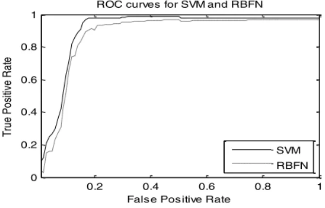
As to the designated fuel consumption model, model output reacts the change of model threshold directly, according to the above, ROC curve is plotted from tracing point of FPR and TPR. Thus, evaluation of model performance is performed through comparison of support vector machine (SVM) and radial basis function network (RBFN). During modeling, 400 samples are selected from flight data sample including full flight phase, 200 samples for training as well as 200 for testing. In RBFN training process, net architecture is initialized to 14-8-1with threshold radial function parameter, and parameter value is adjusted from 1 to 5 gradually. On establishing RBFN model, ROC_RBFN curve is plotted as dotted line in figure 4with the TPR and FPR calculated from RBFN model

output of 200 test samples.

Equally, the adjustable threshold of SVM model is kernel function parameter with its scope from 1 to 20. After establishing SVM model, ROC_SVM curve is plotted as figure 4 in solid line with FPR and TPR proceeded from the

same sample data from SVM model.

0.2 0.4 0.6 0.8 1.0 0 0.2 0.4 0.6 0.8 1 1-s pecificity sens itiv ity

ROC-V curve _{(with c=7)}

0.2 0.4 0.6 0.8 1.0 0 0.2 0.4 0.6 0.8 1 1-s pecificity sens itiv ity ROC-c curve (with V=0.3)

(6)

Fig.4.Comparison of ROC curve between SVM and RBFN

Known from Figure 4, the area under curve of ROC_SVM curve is larger than ROC_RBFN, also we calculated AUC

value to evaluated model performance for both models with non- parameter method[6]. AUC value of ROC_SVM is

0.89, and 0.83 of ROC_RBFN. Obviously, performance of SVM model is better than RBFN model in respect of

classification rate and misclassification rate.

The nature of ROC method for evaluating model performance is the amplification of architecture difference between objective models. The ROC curve plotted with FPR and TPR which are influenced by model output, and insensitive to classifiers. Thus, ROC method has the characteristic of robust. The curve with convex appearance indicates the better model. So ROC curve is suitable for evaluations of evolutionary model. Table 1 illustrates the effect of each optimization period.

Table 1. MODEL PARAMETERS WITH OPTIMIZATION EFFECT

V c r Nsv TPR/% FPR/% CA/% SVM 0.3 5 0.4 18 83.2 21.8 81.4

SVM_V 0.8 5 0.8 11 84.5 15.9 85.8

SVM _c 0.3 13 1.0 13 85.4 16.1 86.3

SVM_V,c 0.8 13 1.3 8 93.8 10.2 95.9

Where r is the distance of SVM soft margin, Nsv is the support vector number; CA is the classification accuracy. Table 1 shows that SVM model which optimized by OOP method has higher performance. Its sensitivity and specificity are significantly improved, and final model SVM_V,c is superior to prototype model, thus it is feasible to

optimize SVM model parameters with OOP method in ROC curve during modeling procedure. Meanwhile, ROC curve is insensitive to the prior knowledge, and this characteristic is helpful for the robustness of model optimization, the statistical significance of this method meets the generalization requirement of SVM algorithm.

4. Model Results

This study introduces an OOP method for optimization of SVM model. The generalization of a trained model involves testing various data sets into the trained neural network to assure the reliability of the fuel consumption estimations. Figure 5 shows the takeoff phase fuel consumption results.

0.2 0.4 0.6 0.8 1 0 0.2 0.4 0.6 0.8 1

Fals e Pos itive Rate

T ru e Po si tive R a te

ROC curves for SVM and RBFN

SVM RBFN

(7)

Fig.5. Distribution of Fuel Flow of SVM Versus Actual

In this figure a plot of actual fuel flow versus modeling output is shown. This representation is typical in flight

performance manuals of civil aircraft. This figure is also known as the flight envelope of the aircraft. The errors

between the estimated and actual fuel burn shown in Figure 5 notes that fuel burn predictions are fairly accurate with a mean estimation error of -0.039% and a standard deviation of 0.307%. It is thus clear that support vector algorithm is feasible for fuel consumption estimate with satisfied accuracy and robust. In full modeling procedure data points are selected so as to include all possible flight conditions, the implementation also extend to full flight phase fuel consumption problem.

5. Conclusion and Recommendations

A representative support vector algorithm aided fuel consumption model is developed using data given in the DFDR and aircraft performance manual. A ROC curve based method for evaluation of SVM is proposed, and an optimization strategy for parameters optimization of SVM modeling is put forward. ROC curve is introduced to evaluate the model performance. The index of area under ROC curve is employed to quantitatively analyze performance of different models, and the validity of this method is verified through case study between SVM and RBFN. Also, the OOP of ROC curve is presented to fix the optimization problem of kernel function parameter and penalty parameter during modeling procedure of SVM, moreover, model generalization is guaranteed by the statistics characteristic of ROC. Finally the support vector sets are trained to estimate fuel consumption of an example aircraft. Results are compared to the actual performance provided in the aircraft performance manual and found to be accurate for possible implementation in fast-time simulation applications.

In future work, the enhancement of the model presented here is the extension to estimate thrust associated with a

fuel burn flight condition parameter such as Thrust Specific Fuel Consumption (TSFC). This parameter is usually a complex function output of march number, temperature, pressure altitude, among other factors. Preliminary results obtained in research indicate that thrust and TSFC can also be easily characterized using support vector algorithm and thus thrust values can be obtained from operational simulation models to support noise studies. Also the large aircraft database application is a challenge work for fuel consumption modeling, although this paper proposed a fuel estimate method for certain aircraft, in actual airlines operation; it is meaningful to apply the current fuel-efficient strategy to fleets with different aircraft type.

Acknowledgment

This paper is supported by National Natural Science Foundation of China (NSFC) under Grant No. 61179066.

0 50 100 150 200 250 1000 2000 3000 4000 5000 6000 7000 8000 Tim e Series /s F uel Cons um pt ion / pph Takeoff Phas e ACTUAL SVM

(8)

References

[1]Alan J. Stolzer. Fuel consumption modeling of a transport category aircraft using flight operations quality assurance data:aliterature review [J]. Journal of Air Transportation, 2002,7(1):93-102.

[2]V.N. Vapnik, An overview of statistical learning theory, IEEE Transactions on Neural Networks, 1999, 10(5):988-999.

[3]Wang Xu-hui, Cao. Li, et al., Lssvm based online trend prediction of gas path parameters of aero engine [J], Journal of Jilin University

2008,38(1):239-244.

[4]Wang xu-hui, Shu ping, Lssvm with fuzzy pre-processing model based aero engine data mining technology [C],International Conference on

Advanced Data Mining and Applications (ADMA '07), Harbin, Springer-Verlag Berlin, 2007, 100-109.

[5]Vladimir Cherkassky, Yunqian Ma. Practical selection of SVM parameters and noise estimation for SVM regression [J]. Neural Networks, 2004, 17(1):113-126.

[6]Bradley A P. The use of the area under the ROC curve in the evaluation of machine learning algorithms [J].Pattern Recognition, 1997, 30:1145-1159.

[7]Wang xu-hui, Shu Ping. A ROC curve method for performance evaluation of support vector machine with optimization strategy [C],

International Forum onComputer Science-Technology and Applications (IFCSTA '09), Chongqing, IEEE CPS, 2009, 117-120.

[8]Robert JG. Determination and interpretation of the Optimal Operating Point for ROC Curves derived through generalized linear models [J]. Understanding Statistics.