Integration of Auxiliary Data Knowledge in Prototype Based Vector Quantization and Classification Models

(1)

Integration of Auxiliary Data Knowledge in

Prototype Based Vector Quantization and

Classification Models

Der Fakultät für Mathematik und Informatik

University Leipzig angenommene

D

ISSERTATION

zur Erlangung des akademischen Grades

D

OCTOR RERUM NATURALIUM

M

ARIKA

K

ADEN (Dr. rer. nat. Marika Kaden)

im Fachgebiet Informatik Vorgelegt von M. Sc. Marika Kaden geboren am 26.07.1985 in Räckelwitz Geburtsname: Kästner

Die Annahme der Dissertation haben empfohlen: 1) Professor Dr. Martin Bogdan (Leipzig) 2) Professor Dr. John A. Lee (Louvain, Frankreich)

3) Professor Dr. Thomas Villmann (Mittweida)

Die Verleihung des akademischen Grades erfolgt mit Bestehen der Verteidigung am 23.05.2016 mit dem Gesamtprädikatmagna cum laude.

(2)

(3)

Bibliographic Descriptions

Kaden, Marika:

Integration of Auxiliary Data Knowledge in Prototype Based Vector Quantization and Classification Models. - 2016. - 195 pages, Leipzig, University Leipzig, Faculty of Math-ematics and Computer Science, Dissertation, 2016

(4)

(5)

Acknowledgement

Thanks to all those which support me on the whole way of learning, studying and working.

First of all my special thank goes to my adviser Prof. Thomas Villmann (Villy). He support me very much and believe in me all my PHD-time. Moreover, I thank Martin Bogdan as my second adviser.

Furthermore, I would like to warmly thank the wholeComputational Intelligence Group of Mittweida especially David Nebel for the lot of discussions, my dissister Tina Geweniger supporting and helping me for further enhancing of the thesis especially improving the English, and mydissisterMandy Lange, who shared the office with me. I also thank the ESF/SAB for financial support.

Last but not least: Thanks to my family and friends: Ganz herzlich möchte ich mich bei meinem Mann Kai-Uwe, meinen Eltern, Schwiegereltern und Freunden bedanken. Alle haben die ganze Zeit an mich geglaubt und mich unterstützt, wo es nur ging. Danke!!! Marika Kaden

(8)

(9)

Symbols and Abbreviations

H Hilbert space

R+ positive real number including zero

NV ∈N number of data point

NW ∈N number of prototypes

NC ∈N number of classes

D∈_N number of dimensions/features

ι∈N iteration step

V ∈_RD _{set of data points}

v∈V data point

v(t)∈V functional data point

W ∈_RD _{set of prototypes}

w∈W prototype

w(t)∈W functional prototype

s(v)∈_N index of the winning prototype forv

Rj(V, W)⊆V receptive field of prototypewj

A grid or lattice (SOM)

wr∈W prototype assigned to neuronr(SOM)

r∈A neuron on the gridA

ˆ

s(v)∈A neuron of the according winning prototype (SOM) C ={1, . . . , NC} set of classes

c(v)∈ C class assignment of a data point

c(v)∈[0,1]NC _{fuzzy class assignment vector of a data point}

ˆ

c(v)∈ C predicted class of a data point y(w)∈ C class assignment of a prototype

y(w)∈[0,1]NC _{fuzzy class assignment vector of a prototype}

d(v,w)∈_R₊ dissimilarity measure ofvandw

dE(v,w)∈R+ Euclidean metric ofvandw

d2_E(v,w)∈_R₊ squared Euclidean dissimilarity measure ofvandw

(10)

κ(v,w)∈_R+ positive semi-definite kernel

lc(v, W)∈_R₊ local cost function

σ∈R+ neighborhood range

θ transfer function parameter (GLVQ)

δi,j ∈ {0,1} Kronecker delta

H(x) Heaviside function

h(x) Delta distribution

SGD StochasticGradientDescent

VQ vectorquantization

uVQ unsupervisedVQ

SOM Self-OrganizingMaps (Heskes)

NG NeuralGas

semi-sVQ semi-SupervisedVQ

LASSO LearningAssociations bySelf-Organization

Tib-LASSO Tibshirani-LeastAbsolutSelection andShrinkageOperator

FLNG/FLSOM FuzzyLabeledNG/SOM

FSNG/FSSOM FuzzySupervisedNG/SOM

sVQ supervisedVQ

LVQ LearningVectorQuantization

GLVQ GeneralizedLVQ

GRLVQ GeneralizedRelevance LVQ

GMLVQ GeneralizedMatrix LVQ

LiRaM LVQ LimitedRankMLVQ

DK-GLVQ DifferentialKernel GLVQ

SVM SupportVectorMachine

SV SupportVectors

RBF RadialBasisFunction

GFR/MLVQ GeneralizedFunctional Relevance/MatrixLVQ

eGR/MLVQ enhancedGeneralizedRelevance/MatrixLVQ

BS-GLVQ border-sensitiveGLVQ

P-GLVQ GLVQwith additive penalty function

AEA AsymmetricErrorAssessment

β-GlVQ,Γ-GLVQ GLVQwith (asymmetric) misclassification costs

ROC-curve ReceiverOperationCharacteristic curve

AUROC Areaunder theROC-curve

(11)

Chapter 1

Introduction

1.1

Motivation and Problem Description

In the last decades, the possibilities of recoding data volumes have been developing rapidly. This development requires new techniques in data processing like storage, reading and analyzing abilities for the huge amounts of data. In this context,Big Data is one of the buzzwords becoming popular in the last years. Yet, an explicit definition of Big Datacannot be found. The term includes the handling of huge data sets in general. Thereby the comprehensions of the wordshandling andhuge depend on the user, his field of research and point in time.

The fact of having such huge data volumes does not only enforce benefit but also challenges especially in the analysis of such data sets. Obviously, manual handling of the data is not longer possible in many applications. Thus, the development of methods which extract essential information from the data shifts more and more into focus. Of-ten, the analyses of large data sets are summarized in the termData Mining. Again, the keywordData Miningdoes not have a clear definition. In general, methods belonging toData Miningsearch systematically for hidden information about and in the data sets. An essential part of the collective termData MiningisMachine Learning(ML) which is an additional tool for classical statistic for data processing. The goal of ML methods is to generate a generalized model of the input data bylearning from examples: In contrast to classical approaches, not an exact physical, chemical or biological model is developed, yet, a model is learned using a given data base. Due to the effectiveness and versatility of applications, the ML methods become important for the analysis ofBig Data.

In general, I distinguish into the three groups of ML methods:

unsupervised Given is a data set. It is searched for a generalized but compressed model describing the data set as close as possible.

supervised Given are input data and output information. Learning takes place as a reduction between predicted and true output of the data. Thereby it is distin-guished between discrete output, the classification, and real output, denoted as regression. Problems, which include both, data with and without output informa-tion, are calledsemi-supervised.

(12)

reinforcement learning A special kind of supervised learning is the reinforcment learning, where the output reward information, i. e. success or non-success, is usually very sparse. This feedback is given after a delay-time only and not imme-diately like in supervised learning.

In this thesis, the focus is put on supervised learning, especially on classification. For this purpose I will utilize basic tools of unsupervised learning. The required details will be described and related to the general (un-)supervised methods in this thesis. For an introduction to reinforcement learning methods I refer to [Sutton and Barto, 1988].

The application of unsupervised ML methods is diverse:

basic analysis Self-organizing Maps [Kohonen, 1982], Hidden Markov Model [Baum et al., 1979]), Generative Topographic Mapping [Bishop et al., 1998],

visualization Principle Component Analysis, Multidimensional Scaling, Stochastic Neighborhood Embedding1

clustering/compressing c-means [MacQueen, 1967], Fuzzy c-means [Bezdek, 1974], Affinity Propagation [Frey and Dueck, 2007], Hierarchical Clustering [Kaufman and Rousseeuw, 1990], Spectral Clustering [v. Luxburg, 2007].

Clustering methods assignsimilardata points to groups of so called clusters. The term similaris task dependent and cannot be defined clearly. Hence, the problem of cluster-ing as well as visualization belongs to the ill-posed problems accordcluster-ing to the definition

ofHadamard[Hadamard, 1902], i. e. the evaluation and comparison of models is not

unique due to the unclear definition ofsimilar.

As for unsupervised tasks, for supervised problems exist a huge number of algo-rithms and methods based on different concepts, e. g.:

Support Vector Machine classification/regression based on convex optimization and learning theory [Schölkopf and Smola, 2002]

Neuronal Network biological inspired classification/regression [Haykin, 1994]

Bayes Classifier classification based on statistical decision theory[Bishop, 2006]

Learning Vector Quantization prototype based methods obtained by combination of Bayes classifier and vector quantization [Kohonen, 1986]

The number of new or extended models for classification is rapidly increasing. One reason thereof is the diversity in the problems. The data bases can be distinguished with regard to many attributes like the number of data samples available for learning, imbalanced class probabilities, class separability, the characteristic, e. g. vectorial data or non-vectorial data, etc. The following two examples illustrate those attributes.

(13)

1.1. Motivation and Problem Description 3

A - remote sensing data A data set may consist of spectra recorded with a hyper-spectral camera over an area. Thereby, reflecting or absorbing spectra are assigned to a pixel representing soil conditions in this area. Here, two specificities regarding clas-sification problems have to be pointed out. First, within the spectra occur correlations depending on the wavelengths/frequencies. Thus, although hyperspectra are usually provided as high dimensional vectors, the problem complexity is much smaller due to these dependencies. The correlations can be incorporated during learning to built up more efficient classification models. Second, in general, a pixel has a resolution of several squared meters on the ground. Hence, a mixture of soil conditions is reflected and thus, a unique class assignment cannot be given. This aspect causes difficulties in classification and is related to this thesis.

B - medical data In medical classifications application a typical task is to assign a diagnosis to a patient record based on measurements, personal data, etc. Frequently, the data basis for model training suffers due to the fact that the number of patients is much lower than the number of healthy persons, i. e. I observe imbalanced class probabilities. For these cases classification models simply optimizing classification accuracy during training might be misleading. Therefore, particularly in medicine, sensitivityandprecisionare favored which should be reflected in the classifier. Further, misclassification costs can be non-symmetric, i. e. a misclassification of a<n healthy person to an unhealthy person might be more costly with respect to side effects or treatment expenses than the other way around. Again, these aspects should be incorporated into the model training.

In general, I believe that those aspects as well as other expert knowledge and a-priori information should contribute to classifier specification to obtain more appropriate and task dependent models. Further, the interpretability of a model gains importance especially in applications.

In this thesis I concentrate on the prototype based classification which originated from unsupervised Vector Quantization. Particularly, I focus on models optimizing well defined criteria comprised in so called cost-functions. This description allows a mathematical precise treatment on the one hand. On the other hand prototype based methods generally allow a good interpretation. Moreover, I will investigate how to integrate expert knowledge in those classifier models. Especially I will consider two types of integration:

I selection and task driven adaption of dissimilarity measures for data comparison

(14)

The functionality of the new investigations is demonstrated on several artificial and real world data sets which are described in the next section.

(15)

1.2. Utilized Data Sets 5

1.2

Utilized Data Sets

The classification problems with underlying data sets are manifold. The kind and char-acteristics of such problems are described in Section. 3. In the following, the data sets used in this thesis are described closer. An overview of the important facts of the single data sets can be found in Table 1.4. Further, it is distinguished between artificial and real world data sets.

Artificial Data Sets

Artificial data sets reflect typical properties of real data sets and the methods should be able to handle them adequately. The design of artificial data sets gives the possibility to demonstrate the specialty of the proposed methods. Further, if the dimensionality of the data is set to two or three, the resulting model can be visualized.

Flags of Palau, Ukraine and Czech

The flags of the nations are very multifaceted regarding colors, symbols, and geometric forms. Therefore, they are well suited for the creation of artificial 2D-data sets with special features and the visualization of the specific ideas of the classification methods. In our case, we use the special characteristics of the flags: Palau, Ukraine and Czech.

Palau-Flag The flag of Palau2 with the derived data set are depicted in Fig. 1.1. The data set consists of two classes and 1099 data points with a class distribution around one to three. The special characteristic of this data set is the non-linear separability in the two dimensional Euclidean space.

Ukraine-Flag The design of the Ukraine flag (see Fig 1.2) is a simple linear separable problem. The data set consists of two class with 1000 data points per class.

Czech-Flag The Czech flag reflects a three class problem (see Fig 1.3), where the classes are pairwise linear separable and touch each other. The number of total data points is 1000.

Triangle

TheTriangledata set consists of two-dimensional data points divided into three classes. Each class is made of 100 equally distributed data samples which are arranged in a rectangle. The special characteristic is the overlap of the pairwise classes (see Fig. 1.4).

(16)

Figure 1.1: Palau data set: original Palau flag (left), derived 2D data set with the two classes+

ando(right)

Figure 1.2:Ukraine data set:original Ukraine flag (left), derived 2D data set with the two classes

+ando(right)

Figure 1.3:Czech data set:original Czech flag (left), derived 2D data set with the three classeso,

(17)

Figure 1.4: Triangle data set: two-dimensional data set with the three classeso,?and+. Each

class consist of 100 data points.

Real world data sets

The novel methods should also work on real world data sets. A special kind of real world data are functional data:

Note 1.1. Functionaldata are data points with lateral dependencies in the neighbored dimensions. In general, we consider vectorsvt∈RD, which are discrete representations of functionsv(t). Examples are time series or spectra.

The following real world data sets, used in this thesis, are described closer. The data sets belonging to different kind of scientific fields like food industry, remote sensing or medicine.

Coffee - hyperspectra from the food industry

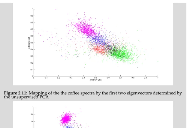
TheCoffee data setcontainsshort-wave infrared range(SWIR) spectra of five different cof-fee types (see Fig. 1.5). The data set is provided by Prof. Udo Seiffert and his research group at Fraunhofer IFF Magdeburg/Germany. The spectra are obtained by utilizing a hyperspectral camera (HySpex SWIR-320m-e, Norsk Elektro Optikk A/S) with the SWIR between 970 nm and 2500 nm at 6 nm resolution yielding 256 bands per spec-trum. Moreover, proper image calibration was done by using a standard reflection pad (polytetrafluoroethylene (PTFE)) [Backhaus et al., 2011]. A data sample is a vector con-taining 256 absorption values. Per coffee type we selected 5000 spectral vectors and normalized them by thel2-norm.

(18)

Figure 1.5:Coffee data set:mean spectra of the five coffee. types

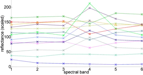
Colorado LANDSAT TM - spectra of remote sensing

The sensors of LANDSAT TM produce images of the ground with seven different spec-tral bands. The resolution of the band1−5 and7 is30 × 30m2 and of band 6it is 60 × 60m2. Thereby, the first three bands are in the visible spectrum (corresponding roughly to the colors blue, green and red) and the bands4,5,7are in the near-infrared spectrum. Thermal band6has a lower spatial resolution and therefore, it was dropped it according to common practice [Augusteijn et al., 1995]. The bands are designed to de-tect and distinguish between different vegetations, rock formations, and other ground characters. The Colorado LANDSAT TM data set3, abbreviatedColorado, is an image of a mountainous region in central Colorado with the pixel size1907 × 1784. The basis of this data set are manually labeled pixels of the image, i. e. each label is ground truth. The ground cover is subdivided into14classes with different occurrences (see Tab. 1.1). The full Colorado data set consists of 3 402 088 data samples with six bands. For training the data set is usually divided into 10%training and 90% test data samples keeping the class distribution. Moreover, the spectra are normalized by thel2-norm.

Further, a second data set is derived. Therefore, I packed10×10pixels of the image to one data sample by averaging the single features and generated fuzzy label vectors. A fuzzy label vectorsc(v)∈[0,1]14contains the percentage of each class in the packed 10 ×10 image. The resulting data set consists of 33 820 data points belonging to a 190×178packed image.

(19)

Figure 1.6: Colorado data set: False color image of a mountainous region in Colorado with 14

different kinds of vegetation or other ground characters (class assignments in Table 1.1).

Indian Pine - spectra of remote sensing

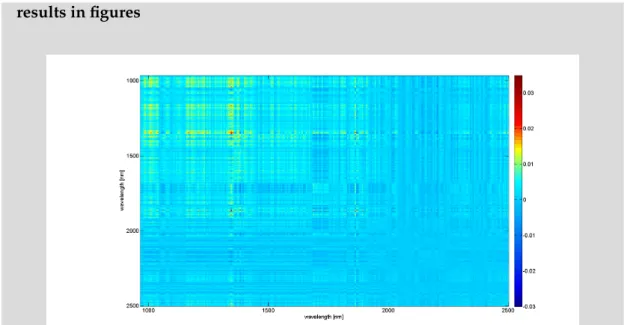
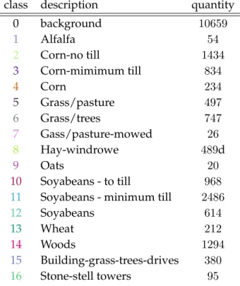
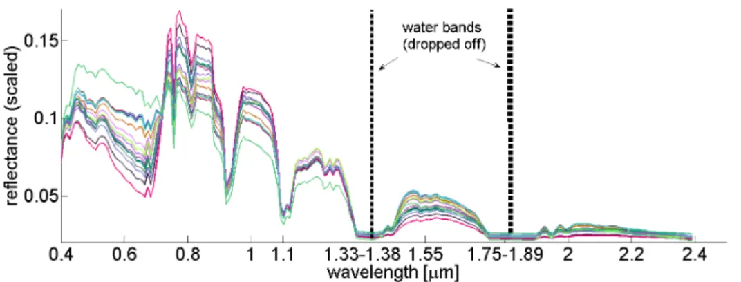
TheIndian Pinedata set4was generated by an AVIRIS sensor capturing an area corre-sponding to145×145pixels in the Indian Pine test site in the northwest of Indiana (see Fig. 1.8, [Langrebe, 2003]). The spectrometer operates in the visible and mid-infrared wavelength range (0.4−2.4µm) with D = 220 equidistant bands. The area includes 16different kinds of forest or other natural perennial vegetation and non-agricultural sectors, which are also denoted as background. These background pixels are removed from the data set as usual. Additionally, we remove20 wavelengths, mainly affected by water content (around1.33µmand1.75µm, see Fig. 1.9). Finally, all spectral vectors were normalized according to the l2-norm. This overall preprocessing is usually

ap-plied to this data set [Langrebe, 2003]. The mean spectra of the16classes are depicted in Figure 1.9.

(20)

Figure 1.7: Colorado data set: mean bands of the 14ground cover classes with the class assignment in Table 1.1.

class description quantity

1 Scotch pine 17.1 %

2 Douglas fir 10.4 %

3 Pine/fir 5.3 %

4 Mixed pine fir 8.0 %

5 Supple/prickle pine 4.3 %

6 Aspen/mixed pine forest 6.1 % 7 Without vegetation 5.0 % 8 Aspen 8.2 % 9 Water 0.5 % 10 Moisten meadow 2.9 % 11 Bush land 3.7 % 12 Grass/pastureland 7.8 % 13 Dry meadow 19.8 % 14 Alpine vegetation 0.8 %

Table 1.1: Colorado data set:name of the classes with the class distribution (color and classes

(21)

Figure 1.8: Indian Pine data set:145×145pixels in theIndian Pinetest site with 16 different

kinds of natural perennial vegetation or non-agricultural areas.

class description quantity

0 background 10659 1 Alfalfa 54 2 Corn-no till 1434 3 Corn-mimimum till 834 4 Corn 234 5 Grass/pasture 497 6 Grass/trees 747 7 Gass/pasture-mowed 26 8 Hay-windrowe 489d 9 Oats 20 10 Soyabeans - to till 968

11 Soyabeans - minimum till 2486

12 Soyabeans 614

13 Wheat 212

14 Woods 1294

15 Building-grass-trees-drives 380

16 Stone-stell towers 95

Table 1.2: Indian Pine data set:name of the classes and class distributions (color and classes

are conformal to Figure 1.8)

Morbus Wilson - medical data set

Morbus Wilson is an autosomal-recessive disorder of copper metabolism. The copper accumulates in the central nerve system, liver and other organs, which leads to dis-turbances in liver function and basal ganglia showing hepatic and extrapyramidal

(22)

mo-Figure 1.9: Indian Pine data set:mean spectra of the16ground cover classes (class assignment see Table 1.2)

tor symptoms. Patients suffering Morbus Wilson develop neurophysiological impair-ments. In the initial non-neurologic phase (NN), impairments are negligible or at least not defacing, whereas later during the neurologic phase (N) the disturbances become severe [Hermann et al., 2003]. During the course of the disease the non-neurological phases manifested in the neurological state. Medical treatment may slow this process down and reduce the symptoms. Depending on the impairment level and the respec-tive pharmaceutical dose rate the treatment causes side effects and could also be expen-sive. Therefore, a precise classification is demanded.

According to a clinical scheme suggested byKonovalov, patients can be divided into two main groups: neurological (N) and non-neurological (NN) [Hermann et al., 2003]. Moreover, these two main groups can be subdivided. The neurological group includes the pseudo-sclerotic (PS), pseudo-parkinsonian (PP) and merged type (MT) subgroup. The non-neurological group can be separated into the hepatic type (HT) and the asymp-tomatic type (AT). A further group consisted of healthy volunteers (V). A clinical (ex-pert) distinction between these subgroups is difficult and requires substantial medical expertise. Different physical examinations are usually applied including among others genetic analysis, fine-motoric, and neuro-physiological tests. The results are condensed in the expert diagnosis by the medical doctor.

There are two different data sets related to Morbus Wilson5:

Morbus Wilson - EIP The impairments of the nervous pathways can be detected by investigation of latencies of evoked potentials collected in a data vector denoted as electro physiological impairment profile (EIP). The Wilson data set EIP contains 122 five-dimensional EIPs described in [Hermann et al., 2003]. The task here is, to classify the patients according to theKonovalov-scheme only on the basis of their

(23)

1.2. Utilized Data Sets 13 class PS PP MT HT AT V EIP2 N NN EIP4 PS PP+MT HT+AT V EIP6 PS PP MT HT AT V number 34 14 8 9 8 47

Table 1.3: Morbus Wilson data set:class subdivisions

iological data. However, it is not clear whether a precise classification based on these data is possible [Hermann et al., 2002].

Three different tasks can be derived from the EIP data set: The first task is to distin-guish between the two main groups only, NN (including V) vs N. A more challenging task is the six-class problem with all the three subgroups. Due to the small number of data samples, we merge several classes (see Tab. 1.3) to obtain a third data setEIP4.

Morbus Wilson - PET The accumulation of copper in the central nervous sys-tem causes a disturbed glucose consumption. To evaluate the smooth transition be-tween the NN and N phase a [18F]-Fluorodesoxyglucose-Positron-Emission-Tomography ([18_F_{]FDG-PET) was applied delivering a neurological impairment profile for each}

pa-tient/proband (see Fig. 1.10) [Hermann et al., 2002].

Thus, the second Wilson data set, denoted asPET, consists of an eleven-dimensional vector containing the normalized glucose consumption in different brain regions (frontal lobe, parietal lobe, temporal lobe, occipital lobe, ant. cingulum, post cingu-lum, putamen, caput nuclei caudati, cerebelcingu-lum, midbrain, thalamic area). This data set can be used to learn a binary classification decision based on the neurophysiological impairment profile. The PET data set contains a non-neurological group (NN) consist-ing 15 volunteers samples and16 non-neurologic samples, and a neurological group (N) of34neurologic samples (N).

Tecator - spectra of the food industry

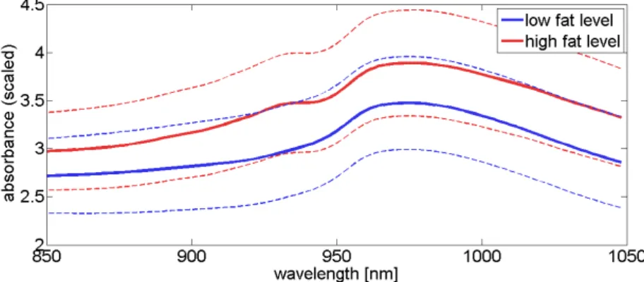
TheTecatordata sets consists of 215 spectra measured for several meat probes. The spec-tral range is850-1050nmwithD= 100spectral bands (see Fig. 1.11). The original data set is labeled according to the fat and protein level. We only use the labels for the fat content and divided the probes between high and low fat level. Further, the data set is provided as a training set (NVtrain = 172) and a test set (NVtest = 43) [Krier et al., 2009].

The data set is available at libraryStaLib6_.

(24)

Figure 1.10: Wilson data set: [18_F_{]FDG-PET analysis: normal (left) and disturbed (right)} [Hermann et al., 2002].

Figure 1.11:Tecator data set:mean absorbing spectra for the two classeshighandlow fatcontent

with their standard deviation (dotted lines).

Wine - spectra of the food industry

Another example from the food industry is theWinedata set which contains121 absorb-ing infrared spectra of wine. The spectra ranges from 4000 - 400cm−1(or equivalently from2.5−25µm) withD= 256equidistant frequency bands (see Fig.1.12). The data are labeled according to the two alcohol levels (low/high) as given in [Krier et al., 2009]. Further, we use the same splitting between training (NVtrain = 94) and test data

(NVtest = 30) as in [Krier et al., 2009]. The spectra with the number 34, 35 and 84 are

identified as outliers and dropped off the data set. The wine data set can be down-loaded from the UCI repository7.

(25)

Figure 1.12:Wine data set:mean absorbing spectra for the two classes. The blue line corresponds

(26)

data set subsets NV D NC normalization characteristic applied Palau- Flag -1099 2 2 -artificial GL VQ, DK-GL VQ Ukraine- Flag -2000 2 2 -artificial BS-GL VQ Czech- Flag -1000 2 3 -artificial P-GL VQ, BS-GL VQ T riangle -300 2 3 -artificial β -GL VQ, Γ -GL VQ Cof fee -25.000 256 5 l2 hyper -spectra GRL VQ, sGRL VQ, GML VQ, DK-GML VQ Colorado all 3 402 088 6 14 -spectral image GL VQ, FSSOM packed 33 820 6 -spectral image with fuzzy labeling FSNG, FSMNG Indian Pine -10 366 200 16 l2 hyper -spectral image eGML VQ Morbus Wilson EIT2 122 11 2 z-scor e clinical trail BS-GL VQ, SVM EIT4 122 11 4 z-scor e clinical trail β -GL VQ, Γ -GL VQ EIT6 122 11 6 z-scor e clinical trail β -FSNG, U -FSNG PET2 65 7 2 z-scor e clinical trail F 2 -GLβ VQ T ecator -215 100 2 -absorbent spectra GFRL VQ W ine -121 256 2 -infrar ed spectr um GRL VQ, GML VQ, sGRL VQ GFRL VQ, sGFRL VQ, eGRL VQ

Table 1.4:Overview of the important facts of the used data sets (NV-number of data points,D

(27)

Chapter 2

Prototype Based Methods for Vector Quantization

Generally speaking, the goal of vector quantization methods (VQ) is to partition of the data space. Vector quantization in the context of Machine Learning is a powerful and essential tool for exploring and investigating the underlying structure of a data set. This thesis concentrates on prototype based methods, i. e. the data are described by representatives also denoted as prototypes. In the followingprototype based VQwe will abbreviated by VQ.

The VQ methods can essentially be divided into unsupervised (uVQ), supervised (sVQ), and semi-supervised (semi-sVQ) methods. One goal among others is to estimate the density distribution of the data set by a few prototypes. Thereby, the data samples together with their (dis-)similarities are given. For unsupervised VQ the cost func-tion, also denoted asexpected risk function, is the quantization error of the model. Well known uVQ methods are the c-means (CM, [MacQueen, 1967]), the Fuzzy-c-means (FCM, [Bezdek, 1974]), the Self-Organizing Maps (SOM, [Kohonen, 1998]), and Neu-ral Gas (NG, [Martinetz et al., 1993]). These methods try to minimize the description error by adapting the prototypes. Thereby, in CM as well as in FCM the prototypes are learned independently [Buttoi and Bengio, 1994]. Yet, SOM and NG are inspired by natural processes and consider additionally the neighborhood cooperation between the prototypes during learning.

Compressing the data by finding data representative prototypes often is only a preprocessing step. Tasks following afterwards are: clustering, visualization of the data set, and further analysis in various areas of application like image pro-cessing, pattern recognition and data mining. Thereby, clustering methods should group given similar data points such that data with related semantical meaning are linked together. A popular prototype based clustering method is Affinity Propagation (AP, [Frey and Dueck, 2007]). Yet, a big issue in unsupervised VQ is the evaluation and interpretation of similarity. Obviously, the evaluation is data-dependent as well as task-dependent. Therefore, clustering and visualization are ill-posed problems. Hence, for cluster solutions exist a lot of validity mea-sures like the Dunn-Index [Dunn, 1973], CONN-index ([Ta¸sdemir and Merényi, 2011], [T. Geweniger and Villmann, 2012]), Cohen’s Kappa [Cohen, 1960] and many more ([Hashimoto et al., 2009], [Zalik and Zalik, 2011]). A lot of them like Dunn- and CONN-index rely on separation and compactness, i. e. it is assumed, that agoodcluster solution

(28)

has compact clusters and the clusters are well separated from each other. Other eval-uation measures are based on further criteria like on information theoretical aspects, e.g. Information Entropy [Bezdek, 1974]. Yet as mentioned before, an optimal cluster solution in general or the one and only measure for model evaluation does not exist.

In the field of supervised VQ, additionally to the data samples the class assignment of each data point is known. It has to be distinguished strictly between training, test and application phase. During the training, a classifier model is adapted on the basis of the training data set using the label information. The evaluation of the model is done on a test set, i. e. labeled data which are not used for training. In the application phase, the classifier model assigns each data point to a class to predict the labels for those new data.

Frequently, the classification error (cerr) or the classification accuracy (acc) is cal-culated for validation during training and test. Thereby, cerr is the number of data points which are misclassified by the model andaccthe number of correct classified data points. However, other statistical quality measures for classification problems can also be used. A few of them are listed in Section 3. In general, a desirable classifi-cation model ends up with a high generalization ability and thus a minimal expected risk, i. e. high performance on data with unknown labels (application phase). Good results on the training set do not imply a goodgeneralization. Roughly speaking, gen-eralizationmeans that a model remains valid for a test data set, i. e. it has similar per-formance like on the training set and avoids learning by heart. Statistical theory about the generalization ability, the Vapnik-Chervonenkis-theory (VC-theory), and how to measure the expected risk, can be found in [Vapnik, 1995]. An alternative description of the generalization ability of a classifier is the Rademacher and Gaussian complexity [Bartlett and Mendelson, 2002]. Although the classification task seems to be well de-fined, the goal and condition in several application methods differ, which leads to a large number of classifiers. A more detailed description of these aspects is addressed in Section 3.

Cluster methods may also be adapted to be used also for classification. Thereby, after uVQ and clustering of the prototypes, the prototypes are post-labeled. Note, a good cluster solution does not imply a good classification error or the other way around. Thus, beside the data samples the label information should be incor-porated during the learning like in Supervised Neural Gas [Villmann et al., 2003] or in semi-supervised classification methods e. g. the Fuzzy Labeled Neural Gas (FLNG, [Villmann et al., 2006b]) or the Fuzzy Supervised Neural Gas (FSNG, [Kästner and Villmann, 2012]). In semi-supervised leaning both labeled and unlabeled data are given. The unlabeled data also contribute to build a model for improving the classification outcome.

(29)

19 the data. We definedistanceordissimilaritymeasures as follows:

Note 2.1. In this work, we use the same denotation as given in Pekalska&Duin

[Pekalska and Duin, 2005]. Ametricd :RD ×RD → R+fulfills the following

require-ments forx, y, z ∈_RD

reflexivity d(x, x) = 0

symmetry d(x, y) =d(y, x)

definiteness d(x, y) = 0⇒x=y

triangle inequality d(x, y) +d(y, z)≤d(x, z) .

Ifd(x, y)is not a metric, we distinguish betweenhollow,pre-,quasiandsemimetrics (see Tab. 2.1). Unless stated otherwise, the notationsdistanceor dissimilaritymeasure refer to the hollow metric, i. e. only the reflexivity has to be fulfilled.

reflexivity symmetry definiteness triangle equation

hollow metric x - -

-pre metric x x -

-quasi metric x x x

-semi metric x x - x

Table 2.1: Different kinds of dissimilarity measuresd:_RD_×

RD→R+

In the following a few prototype based unsupervised, supervised and semi-supervised vector quantization methods will be introduced in their basic variants. Later on some of these will be extended and improved.

(30)

Parts of the section are based on

T. Geweniger, L. Fischer, M. Kaden, M. Lange and T. Villmann: Clustering by Fuzzy Neural Gas and Evaluation for Fuzzy Clusters. Computational Intelligence and Neu-roscience, 2013.

2.1

Unsupervised Vector Quantization

Prototype based uVQ uses a set of prototypesW ={w1, . . . ,wNW} ∈R

D _{to represent}

a vectorial data setV = {v1, ..,vNV} ∈ R

D_{. In crisp VQ, an index mapping function}

Υ :IV ={1, . . . , NV} 7−→IW ={1, . . . , NW}maps the indexiof each data pointvito

an indexjof a prototypewj. In fuzzy VQ, this index mapping is not unique, i. e. a data

pointvican be assigned to several prototypes (cf. page 29). First, we consider crisp VQ.

Each data pointviis assigned to a prototype by thewinner-takes-all(WTA) rule:

i7−→j=s(vi) = argmin k∈IW

(d(vi,wk)) , (2.1)

such thats(vi)refers to the index of the best matching prototype in terms of the distance

functiond(vi,wj). The distanced(vi,wj)describes the dissimilarity betweenviandwj.

Oftend(v,w)is based on the Euclidean norm

dE(v,w) =||v−w||E = v u u t D X k=1 (vk−wk)2 (2.2)

or the squared Euclidean distance

d2_E(v,w) = (dE(v,w))2 = D

X

k=1

(vk−wk)2. (2.3)

It has to be mentioned that the squared Euclidean distance not a metric, i. e. it is a quasi metric (see Note 2.1). Furthermore, any other dissimilarity measure such as the Sobolev distances, divergences, thelp distances, or kernel distances can be applied depending

on the applications and the VQ model. We will discuss deeper details about distance or dissimilarity measures in Section 2.4.

The WTA rule (2.1) realizes a partition of the data space into Voronoi cells, denoted as receptive fields in prototype based VQ. Each receptive field

Rj(V, W) ={v∈V|d(v,wj)≤d(v,wk)∀j6=k} (2.4)

(31)

2.1. Unsupervised Vector Quantization 21 the receptive fields1are:

NW [ k=1 Rk(V, W) =RD and µ NW \ k=1 Rk(V, W) ! = 0

where math measureµ(M) = 0implies that the setM is of the measure zero.

As already mentioned, the goal of uVQ is, among others, to minimize the description error. This can be modeled by the following general continuous cost function:

EuV Q=

Z

P(v)·lc(v, W) dv (2.5)

whereP(v) is the data density andlc(v, W) are thelocal costs. Thereby, each method has its own specific local cost function. If it is set to lc(v, W) = d2_E(v,ws(v)), EuV Q

describes the common quadratic Euclidean description error.

Unsupervised VQ is an unconstrained, in general non-linear and non-convex opti-mization problem. Thestochastic gradient descent (SGD) strategy is a well established method solving this kind of cost function based optimization problems. The SGD is applied on several other cost functions mentioned in this work. The selection of this optimization strategy has an historical background. A more detailed description of SGD can be found in appendix A.1. In the following, in oneepochιof SGD all data are considered once in a random sequence. The general update in uVQ of the prototypes

wjcan be determined by:

wj ← wj−α·∆wj (2.6)

∆wj ∼

∂ lc(v, W)

∂wj

, (2.7)

where0 < α ≪1is the learning rate2. The SGD is performed until convergence, i. e. the change of the outcome of the cost function is smaller than a predisposed value, or until a predefined number of epochs is reached.

For the data compression task, the number of prototypes has to be very small com-pared to the number of data points, i. e. NW ≪NV. The existing cost function based

VQ methods differ in the definition of the local costs. Several models are motivated by neural data processing in the brains whereas other are inspired by physics.

1_{We assume data densities without Dirac impulses.} 2_{The parameter}_w

jis a vector. The gradient ∂d(v,wj)

∂wj is a shorthand notation for a vector with entries of the single derivatives∂d([v]l,[wj]l)

(32)

2.1.1 C-means

Many advanced methods are based on the c-means method introduced first by

MacQueen[MacQueen, 1967]. The goal of c-meansis to partition the data space into

cclusters such that the sum of the distances of the data samples to the cluster means is minimal. The local costs in (2.5) are defined by

lcCM(v, W) =d(v,ws(v)), (2.8)

where in the original work of MacQueen d(v,w) is the squared Euclidean distance. The learned prototypeswj can interpreted as centroid in the contentious and as cluster

means in the discrete case. The number of prototypes, i. e. the number of clustersc, has to be chosen in advance.

Finding the minimum of the cost function (2.5) with the local costs (2.8) isNP-hard. As already mentioned, the SGD can be applied to find a local minimum of the cost function. In each iteration step, where one randomly chosen data pointvis considered, only the best matching prototype ws(v) is adapted. The update of prototype ws(v) is

obtained by the partial derivatives of the cost function according tow_s₍_v₎:

ws(v)←ws(v)−α·

∂ d v,ws(v)

∂ws(v)

,

where 0 < α ≪ 1 is the learning rate and has to be decreased during the learning process.

Recent studies for c-means replace the squared Euclidean distancesd(v,w)by further distance measures [Karayiannis and Randolph-Gips, 2003]. Yet, the distance function has to be differentiable according to the parameters, i. e. to the prototypes.

Although, CM is known to find only local optima [Bottou and Bengio, 1994], it is widely used. To overcome this locality behavior, the algorithm is usually performed several runs with different initializations and the best achieved model is taken. An-other problem of CM is the occurrence of dead units. Dead units are never winning prototypes wj, i. e. j 6= s(v) ∀v ∈ V. An alternative to assure a faster convergence,

avoid local optima and dead units is to include local neighborhood cooperativeness between the prototypes as outlined in the following.

2.1.2 Self-Organizing Map

The Self-Organizing Map (SOM) is introduced for efficient VQ inspired by cortical maps as well as data visualization by Kohonen ([Kohonen, 1982], [Kohonen, 1998]). The neighborhood cooperativeness in Kohonen-SOM is inspired by cortical sensory maps in the human brain, i. e. similar stimulus mapped spatially to neighbored neu-ronal structures. This principle is modeled by topology preserving mapping from a

(33)

D-2.1. Unsupervised Vector Quantization 23 dimensional data space V onto a low-dimensional simple geometric gridA (typically two or three dimensions). Thereby, each prototypewr ∈RD is assigned to a node also denoted asneuronr ∈ A. Generally, the geometric gridAis fixed and the prototypes

wrare adapted according to the neighborhood cooperativeness inA.

A lot of modifications, extensions and mathematical analyses of theKohonen-SOM are published ([Heskes, 1999], [Vesanto, 1999], [Kaski et al., 1998], [Kohonen, 2013]). The original SOM byKohonenis not based on a cost function [Erwin et al., 1992]. One fundamental improvement was presented byHeskes[Heskes, 1999] who established a modified SOM based on a cost function keeping the main idea of Kohonen-SOM neighborhood cooperativeness. The cost function introduced byHeskeshas the same structure as (2.5). However, the local costs are defined via:

lcSOM(v, W, σ) = X r0_∈_A

hSOM_σ ˆs(v),r0

d(v,wr0), (2.9)

taking into account the topological structure of the external gridA. In opposite to the WTA-rule (2.1), the winner in (2.9) is determined by:

ˆ s(v) = argmin_r∈_A X r0_∈_A hSOM_σ r,r0 d(v,wr0) ! (2.10)

depending on the neighborhood function hSOM_σ r,r0 = exp −dA(r,r 0₎ 2σ2 (2.11) evaluate inA. The valueσ >0determines the influence range in the lattice. It has to be pointed out: the neighborhood functionhSOM

σ and, therefore, the winner determination

ˆ

s(v)take into account the distancedA(r,r0)of the neurons in the external latticeA. The

distancedAdepends on the type of A, e.g. in general, if the grid is rectangular,dAis the

Manhattan metric or if A is hexagonal,dAis chosen as Euclidean distance.

The optimization of the cost function (2.5) with the local costs (2.9) by SGD leads to the learning rule

4wr ∼ −hSOMσ (r,ˆs(v))

∂d(v,wr) ∂wr

. (2.12)

It should be emphasized that this derivation of the gradient descent learning is only valid iff the local costslcSOM₍_v_{, W, σ}₎_{in the cost function (2.5) are exactly the same as}

those used for the winner mapping in (2.10) [Villmann, 2006].

Besides compressing and clustering the information while preserving the basic topo-logical and metric relations, the main virtue of the SOM is its visualization ability. The clustering solution becomes visible with the projectionΥSOM :IV 7−→A. An overview

(34)

of visualizations methods are given in [Vesanto, 1999]. Two well-established visualiza-tion tools for SOM models with a two dimensional latticeAare:

Component planes A component plane coded for each neuron in this lattice is the value of one dimension or also called component[wr]k. This value is coded by a

color scale or gray levels. Thus, the number of component planes is identical with the number of dimensions. The component planes may give a hint whether the SOM model is topology preserving [Vesanto, 1999, Villmann, 2006]. An example is depicted in 2.1.

U-matrix The U-matrix was developed byUltsch[Ultsch and Semon, 1990] and is a distance matrix based on the SOM-lattice. For each neuronrthe direct neighbors in the grid taken as graph are determinedN N(r), e. g. in the rectangular lattice these are four for the neurons inside the lattice and, accordingly fewer for neurons at the border. In the U-matrix the distanced(wr, wr0)is visualized by using a gray level scale or component planes, respectively. Thus, the size of the u-matrix for a rectangular lattice with the sizea×bis(2·a−1)(2·b−1). A generalization thereof is: each neuron is attached by a third dimension called the u-high. This u-high codes the mean distance of a neuron to its direct neighbors:

u(r) = 1 |N N(r)|

X

r0_∈_{N N}₍_r₎

d(wr,wr0)

The u-matrix is a powerful tool for the interpretation of the resulting model. It also can be used to determine the number of clusters [Ultsch and Semon, 1990]. An exemplified U-matrix is shown in Fig. 2.2.

Crucial issues concerning the structure of the SOM-lattice are: • number of nodes

• neighborhood structure and • shape of the grid.

These questions are data depending and there exists no general answer. The re-sulting model should be checked, whether the SOM solution is topology preserving [Villmann, 2006]. If the model is topology preserving, the result should be used for further analyses and conclusions. Thus, the fixed prior chosen lattice causes topologi-cal restrictions and therefore, can induce difficulties in applications. A further method with natural visualization ability which also relies a data depended lattice (not fixed beforehand) is theTopology Representing Network. A description thereof can be found in [Martinetz and Schulten, 1994]. A further alternative is theNeural Gas, which is expli-cated in the next part.

(35)

2.1. Unsupervised Vector Quantization 25

Figure 2.1: Component planes for the six features of the Colorado data set (see page 8). The

rectangular grid size is6×7.The component planes show a good behavior of the SOM-model. This is also reflected in the topographic product of−8.7·10−4_≈₀_{[Villmann, 2006].}

(36)

2.1.3 Neural Gas

The Neural Gas (NG) was introduced by Martinetz, Berkovich, & Schulten

and is inspired by the SOM [Martinetz et al., 1993]. In Neural Gas a neighborhood co-operativeness between prototypes is also integrated in the local cost to speed up the convergence compared to CM. Yet, the NG neighborhood functionhN G_σ is evaluated in the input spaceV and not on an external grid like in SOM. More precisely,hN G_σ depends on thewinner rank function

rkj(v, W) = NW X k=1 H(d(v,wj)−d(v,wk)) (2.13) where H(x) = ( 0 if x≤0 1 else (2.14)

is the Heaviside function. The winning prototypew_s₍_v₎has the rankrk_s₍_v₎(v, W) = 0, the second closest prototypewjthe rankrkj(v, W) = 1and so one. The neighborhood

function yield to:

hN G_σ (rkj(v, W)) = exp −rkj(v, W) 2σ2 (2.15) with the neighborhood rangeσ ≥ 0. For σ > 0, beside the winning prototypews(v)

also the prototypes of higher ranks are updated. In general,σslowly decreased to zero during learning [Martinetz et al., 1993].

The local costs are:

lcN G(v, W, σ) =

NW

X

j=1

hN G_σ (rkj(v, W)) d(v,wj) (2.16)

and the cost function of the neural gas yields to: ENG(V, W) =

1

C(σ) Z

P(v)lcN G(v, W, σ)dv (2.17)

with data densityP(v)and the normalization constantC(σ) = PNW

j=1hN Gσ (rkj). The

cost function corresponds to the energy function of a gas with the particlesw, the po-tentialV and the viscosityσ.

The learning takes place as stochastic gradient descent onEN Gaccording to

wj ← wj −α∆wj (2.18)

∆wj ∼ hN Gσ (rkj(v, W))·

∂d(v,wj)

∂wj

(37)

2.1. Unsupervised Vector Quantization 27 where α > 0 is the learning rate. During the adaptation process the shifting of the prototypes can be interpreted as the dynamic of the diffusing particles moving in a potential determined by the data density [Martinetz et al., 1993].

In a nutshell, the NG is an efficient tool for uVQ. Like SOM the NG takes also the neighborhood cooperativeness into account. Thus, the method is not sensitive to the initialization like c-means and therefore is robust. Further, due to the neighborhood cooperatives dead units are avoided. Compared to SOM, an advantage is the abolition of the topological restriction in the neighborhood cooperativeness because of the win-ner ranks. Therefore, Neural Gas is a good choice for unsupervised vector quantization problems. Yet, NG does not provide a feasible possibility for visualization.

2.1.4 Common Generalizations

So far only the basic prototype based uVQ methods were explained. Yet, there exist a lot of extensions and modifications. A few of them are summarized in this section and exemplified on the Neural Gas method.

Batch Variants

In the last section only theonlinevariants of the uVQ were presented, i. e. during each prototype update step only one data point is taken into account. The notation batch indicate another optimization strategy. Though, for an averaged update of the pro-totypes all data points are taken into account in one iteration step and therefore, all data points have to be presented in advance. In general, an alternating optimization scheme adapted from the Expectation-Maximization strategy (EM, [Bishop, 2006]) is applied and in each iteration step prototypes are set to an weighting average over the data samples (Batch c-means [Ball and Hall, 1967], Batch SOM [Cheng, 1997], Batch NG [Cottrell et al., 2006]).

Batch NG For Batch NG the discrete form of the NG cost function is defined by

ENGdisc(V, W) = 1 C(σ) NV X i=1 lcN G(vi, W, σ) (2.20)

with the local costslcN G(vi, W, σ)from (2.16). The ranks are interpreted as hidden

vari-ableskji=rkj(vi, W)where the vectorski ={kji∈ {0, . . . , NW−1}|vi ∈V}constitute

a permutation of the set{0, . . . NW −1}and includes all winner ranks. Thus, the new

parameters of the cost function (2.20) arekiandwj. The optimization ofENGdisc(V, W)

might be done by an alternating optimization strategy [Bishop, 2006], which consist of the following two alternating adaptation steps:

(38)

step A Calculate the ranks ofwjfor all data points: kji = NW X k=1 H(d(vi,wj)−d(vi,wk))

step B Fix the parameter vectorki. Update prototypewj by the weighted average:

wj = PNV k=1hN Gσ (kjk)·vi PNV k=1hN Gσ (kjk) (2.21)

Step B can be interpreted as a second order optimization according to Newton opti-mization. The derivation of the formula (2.21) can be found in [Cottrell et al., 2006]. It has to be mentioned that this batch variant is formulated for the squared Euclidean distance. The distanced2_Eis implicitly involved in (2.21).

The Batch SOM is analog to the Batch NG, only the neighborhood function and the winner determination is changed accordingly [Cheng, 1997]. Usually, only a few adap-tation steps are necessary for convergence in the batch variants [Cottrell et al., 2006].

In general, the batch variants are faster in convergence especially on high dimen-sional data, because only one adaptation is necessary in each epoch. However, the prototypes might get stuck in local minima and in particularly in Batch SOM, the prob-lem of topological mismatches and the dependency on the initialization is much more pronounced as for online learning [Fort et al., 2001].

Median and Relational Variants

In some fields of application like in the analysis of protein structures and text docu-ments, the data are not given in the standard Euclidean vector space. Instead, a discrete representation of the data or even only a (dis-)similarity matrix are available. In these cases the standard shifting (2.6) of the prototypes is not possible due to the derivations ofd(v,w)do not exist.

In the median variants the prototypes are restricted to be data points, i. e. an in-dex mapping Ψ : l ∈ {1, . . . NW} 7−→ ˜l ∈ {1, . . . NV} is learned (Median NG

[Cottrell et al., 2006], Median SOM [Kohonen and Somervuo, 2002]). Hence, only the dissimilarity matrixD∈ _RNV×NV

+ of the data points has to be given. Moreover,Dhas

to be a quasi metric3[Cottrell et al., 2006].

Extensions of the median variants are the relational methods, where the prototypes are assumed to be linear combination of the data points w = PNV

i=1αivi. Thus, the

linear factorsαi are adjusted during the learning (Relational NG [Cottrell et al., 2006],

3_{The dissimilarity measure}_D_{can be embedded in a pseudo-Euclidean vector space (see Note 2.1 or} [Pekalska and Duin, 2005]).

(39)

2.1. Unsupervised Vector Quantization 29 Relational SOM [Hasenfuss and Hammer, 2007]). Like in the median variants, only the dissimilarity matrix D has to be given and which has to be a quasi metric [Hasenfuss, 2009].

Median NG In Median NG ([Cottrell et al., 2006]) a prototype wl is mapped on a

data point v˜_l with d_i˜_l = d(vi,v˜_l). To learn this index mapping step B for Batch NG

(2.21) is replaced by: ˜ l← argmin l0_∈{₁_,...,N V} NV X i=1 hN G_σ (kli)di,l0

with the fixed vectorki={kli ∈ {0, . . . , NW −1}|vi ∈V}.

Fuzzy Variants

Until now the assignment of a data pointvito a prototypewjis unique and crisp. Let,

U ∈ _RNV×NP

+ be an assignment matrix and in fuzzy variants of uVQ (fuzzyVQ) these

assignmentsuij can be possibilisticuij ∈[0,1]or probabilistic (uij ≥0andPNj=1W uij =

1). For crisp VQ yieldsuij = 1ifviis mapped towj anduij = 0otherwise.

The discrete cost function of the fuzzyVQ variant has the form:

Ef uzzyV Q= NV X i=1 NW X j=1 um_ij ·lc(vi,wj, W) (2.22)

where lc(vi,wj, W) are the local costs and m is the fuzzyness parameter usually set

between 1.2 ≤ m ≤ 2 [Bezdek, 1980]. If m → 1, the assignments converge to the crisp solution and for m → ∞ a unique distribution is forced [Bezdek, 1980]. For fuzzyVQ variants, both the position of the prototypes and the assignments uij have

to be adapted. Frequently, the learning of both parameters is done by alternating op-timization [Bezdek and Hathaway, 2003]. This opop-timization principle is similar to the batch variants.

The Fuzzy-C-Means (FCM) was proposed byDunn[Dunn, 1973] and elaborately dis-cussed and improved byBezdek[Bezdek, 1980]. Later, the idea of fuzzyness was trans-fered to the SOM (FSOM [Tsao et al., 1994]) and NG (FNG [Geweniger et al., 2013]). Again, we specify the basic principle for NG.

Fuzzy Neural Gas The cost function of the Fuzzy Neural Gas (FNG) yields to:

EF N G= NV X i=1 NW X j=1 um_ij ·lcF N G(vi,wj, W, σ) (2.23)

(40)

withlcF N Gsimilar to the local costs of the original NG (2.16): lcF N G(v,wj, W, σ) = NW X l=1 hF N G_σ (rkj(wl, W)) d2E(v,wj). (2.24)

Yet, the rank is determined according to the best matching prototype and not according to the data points:

hF N G_σ (rkj(wl, W)) = exp −rkj(wj, W) 2σ2 (2.25) is the neighborhood function of the FNG with the winner rank function

rkj(wl, W) = NW X k=1 H d2_E(wl,wj)−d2E(wl,wk) . (2.26)

Analog to Batch NG, the optimization of the FNG cost function with the parameters prototypeswand fuzzy assignmentsum_ij instead of the hidden variableskjis based on

the alternating optimization strategy. Thus, we obtain the following steps, which have to be processed alternatingly:

step A Calculate the fuzzy assignmentsuij for all data points:

uij = 1 PNW l=1 (lcF N G(v,wj, W, σ)) 1−m_· (lcF N G₍_v_,_w l, W, σ))m −1

step B Fix the fuzzy assignmentsuij and update prototypewj: Using the squared

Eu-clidean distance the update equation can be formulated as:

wj = PNV i=1 PNW l=1 umil ·hF N Gσ (rkj(wl, W))·vi PNV i=1 PNW l=1 umil ·hσF N G(rkj(wl, W)) (2.27)

A more detailed description and the proof of convergence can be found in [Geweniger et al., 2013].

(41)

2.2. Supervised Vector Quantization 31

2.2

Supervised Vector Quantization

As already mentioned, for sVQ beside the training samplesv∈V ⊂RD also the class assignmentsc(v)∈ C ={1, . . . , NC}are given. The task is to find a model which assign

a data pointvto a predicted labelˆc(v) ∈ C under the aspect of correctness, i. e. good classification performance.

A common measure to evaluate the classification performance is the classification accuracyacc(V, W)or the classification errorcerr(V, W), respectively. The accuracy is determined by the relative number of data points which are classified correctly by the model, i. e.: acc(V, W) = 1 NV X v∈V δc(v),ˆc(v) (2.28)

whereδi,jis the Kronecker delta with

δi,j =

(

1 , ifi=j

0 , else (2.29)

The classification error is simplycerr(V, W) = 1−acc(V, W).

Two well known prototype based classifier models are the Support Vector Ma-chine (SVM, [Schölkopf and Smola, 2002]) and the Learning Vector Quantization (LVQ, [Kohonen, 1998, Sato and Yamada, 1996]). The SVM is an extension of a hyperplane classifier to solve non-linear separable binary classification problems. The hyperplane is described by the prototypes, called Support Vectors, and therefore, the prototypes are class border typical. The cost function of the SVM maximizes the margin between two classes and is model as quadratic optimization problem with convex constraints. It has to be pointed out that the SVM is a binary classifier. Extensions to multi-class problems are only based on heuristics. A more detailed description can be found in the Appendix A.2 or in [Schölkopf and Smola, 2002].

The Learning Vector Quantizers are well established Bayesian classifiers with an in-tuitive learning principle. A detailed description of the LVQ methods follows.

2.2.1 The Family of Learning Vector Quantizers - LVQ

The basic method LVQ 1 was introduced byKohonenwith the goal to approximate a Bayesclassification scheme in an intuitive manner [Kohonen, 1986]. At the beginning of the training phase data pointsv∈V with their labelsc(v)and at least one initialized prototypewper class withy(w)∈ Care given. LVQ 1 is based on the Hebbian learning scheme and is an iterative method. In one iteration step a data pointvis chosen ran-domly and the nearest prototype, the winnerws(v), is determined using the squared

(42)

Euclidean distanced2_E (2.1). The update of the winnerws(v)

ws(v)←−ws(v)−α·∆ws(v) (2.30)

depends on the label matching

∆w_s₍_v₎ = (−1)1+δc(v),y(w_s₍_v₎₎_·

(v−w_s₍_v₎)

where0< α1is a decreasing learning rate. The adjusting of the prototypes follows the intuitive principle ofattraction and repulsing:

attraction If the winning prototype w_s₍_v₎ is of the same class as the presented data pointv, i. e.c(v) =y(ws(v)),ws(v)will be attracted due to:(−1)

1+δc(v),y(w_s₍_v₎₎

= 1.

repulsing If the label of the winning prototypew_s₍_v₎is different compared toc(v), the prototype will be pushed away, i. e.(−1)1+δc(v),y(ws(v)) ₌₋₁_.

At the end of the training, the prototypes should describe their classes as precise as possible.

The assignment of a data point with an unknown label is done by nearest prototype classification (NPC):

N P C : y(ws(v))7→ˆc(v). (2.31)

The simple principle of LVQ is very effective in a lot of applications ([Umer and Khiyal, 2007], [Bashyal and Venayagamoorthy, 2008]). However, there are some disadvantages, like slow convergence or instability in some cases: If prototypes and data points are in an inappropriate constellation e. g. unbalanced data or unfa-vorably initialized, the prototypes might be pushed away always. Therefore, some improvements are developed, e. g. LVQ 2.1 and LVQ 3 [Kohonen, 1998].

LVQ 2.1 For LVQ 2.1 beside the winning prototypews(v)also the second best

match-ing prototypews2(v)with

s2(v) = argmin

k∈{1,...,NW},k6=s(v)

d(v,wk) (2.32)

is considered. Thereby, the update of these prototypes has to be distinguished into three cases:

case I c(v) = y(w_s₍_v₎) = y(w_s₂₍_v₎): No update is performed because of the robust decision.

(43)

2.2. Supervised Vector Quantization 33

case II c(v)6=y(ws(v))andc(v)6=y(ws2(v)): Both prototypes are pushed away

∆ws(v) = −α·(v−ws(v))

∆ws2(v) = −α·(v−ws2(v)).

case III k, l∈ {s(v), s2(v)}andk6=l: Ifc(v) =y(wk)6=y(wl)and both prototypes are

located within thewindow

min (v−wl) 2 (v−wk)2 ,(v−wk) 2 (v−wl)2 ! > 1−ω 1 +ω , (2.33)

the prototypewkis attracted andwlis pushed away

∆wk = +α·(v−wk)

∆wl = −α·(v−wl).

The window parameter0 < ω ≤1effects the number of training samples taking into account during the learning. A good choice forωis0.2to0.3[Kohonen, 1998]. The window rule assures that only prototypes around the decision border are considered, without this rule the prototypes may diverge.

The LVQ 2.1 should be applied subsequently to LVQ 1 and run for only a few iteration steps, because it may cause instable behavior [Kohonen, 1998]. If we consider only one prototype per class, LVQ 1 tries to arrange the prototypes in the class centers. Other-wise, LVQ 2.1 is more class border sensitive, because of window rule (2.33).

LVQ 3 The variant LVQ 3 is based on LVQ 2.1 and only differs incase I. Hereby, both prototypes are attracted:

∆ws(v) = α·(v−ws(v))

∆ws2(v) = α·(v−ws2(v))

The LVQ 3 should only be applied in addition to LVQ 1 like for LVQ 2.1

All mentioned heuristics and combinations thereof typically have a good perfor-mance in practical applications. However, they are only heuristics and, therefore, no predictions about the learned models and local or global optima are possible. An ex-tended version is the Generalized Learning Vector Quantization which is based on a cost function and, therefore, is mathematically more sound.

(44)

2.2.2 Generalized Learning Vector Quantization

The Generalized Learning Vector Quantization (GLVQ) was introduced bySato and

Yamadain 1995 [Sato and Yamada, 1996]. The goal of the GLVQ method is to minimize

the classification error by keeping the principle of prototype learning known from LVQ. For that purpose,Sato and Yamadaintroduced theclassifier function:

µW(v) =

d+(v)−d−(v)

d+₍_v_{) +}_d−₍_v₎, (2.34)

whered+(v) =d(v,w+)is the distance between data pointvand its the best matching prototypew+ with the same label, i. e. c(v) = y(w+). Otherwise, d−(v) = d(v,w−) is the distance between data pointvand the closest, wrong labeled prototypew−, i. e. c(v)6=y(w−). More precisely: w+ = argmin w∈W+₍_v₎ d(v,w) with W+(v) ={w∈W |y(w) =c(v)} (2.35) w− = argmin w∈W−₍_v₎ d(v,w) with W−(v) ={w∈W |y(w)6=c(v)} (2.36)

Obviously, the classifier function (2.34) is non-positive iff the data point is correct clas-sified, i. e. d+₍_v₎ _≤ _d−₍_v₎ _{is valid. Due to the normalization term}_d+₍_v_{) +}_d−₍_v₎_the range ofµW(v)is in the intervalµW(v)is[−1,1].

The cost function is a soft version of the classification error and has the form of: EGLV Q= 1 NV X v∈V fθ(µW(v)) (2.37)

with thetransfer functionfθ. The transfer function has to be monotonically increasing.

Common choices are the identity or the sigmoid function fθ(x) =

1

1 +e−θ·x. (2.38)

which depends on the parameterθ. Choosing the latter one, the range of the sum terms in (2.37) is[0,1]and, hence, the cost function approximates the classification error for θ% ∞(see Sec. 5.1).

The minimization of the differentiable cost function (2.37) can be done by stochastic gradient descent. The update rules result in

w±←w±−αW

∂EGLV Q

(45)

2.2. Supervised Vector Quantization 35 with learning rate0< αW 1and derivatives

∂EGLV Q ∂w± = ξ ± θ (v)· ∂d±(v) ∂w± (2.40) with ξ_θ±(v) = f_θ0(µW(v))· ±d∓(v) (d+₍_v_{) +}_d−₍_v₎₎2 . (2.41)

As it can be seen in (2.40), the updates depend on the derivatives of the distance mea-sure according to the prototypes. Therefore, one requirement on the distance meamea-sure is the differentiability. A common choice is the squared Euclidean distance which ends up in a vector shift of the prototypes during the update:

∂d±(v)

∂w± =−2(v−w

±

). (2.42)

It turns out, the GLVQ with squared Euclidean distance and optimization by SGD is alike the LVQ 2.1 with data dependent factors in the update (see Sec. 5.1).

The GLVQ belongs to the margin optimizers like the SVM. Yet, the GLVQ optimizes the hypothesis margin1₂(d+₍_v₎₋_d−₍_v₎₎_{[Crammer et al., 2003]. The hypothesis margin} is related to the distance a prototype can be altered without changing the classification decision. Thus, this fact indicates an efficient structural risk optimization in the learning phase [Hammer et al., 2001]. Further, in case of overlapping classes the GLVQ is more robust than LVQ, since convergence is assured.

Moreover, LVQ or GLVQ are flexible related to the distance measures: any dissimi-larity measure which is differentiable according to the prototypes can be applied and distance adaption is also feasible (see Sec. 2.4).

Further, GLVQ is designed for multi-class problems, i. e. NC >2. The only

require-ment is to provide at least one prototype per class and therefore, the complexity of the resulting model has to be determined in advance. The correct number of prototypes is hard to identify and depends on the data set. However, less is more: In many applica-tions one prototype per class is adequate if additionally distance adaption is applied ([Biehl et al., 2012],[Biehl et al., 2013]). Note, if the standard GLVQ with Euclidean dis-tance and one prototype per class is performed, it is equivalent to a linear classifier.

Analog to the methods for unsupervised VQ, different variants of GLVQ are avail-able: Median GLVQ [Nebel et al., 2013], Relation GLVQ [Hammer et al., 2011] and also fuzzy variants [Villmann et al., 2008]. Further, probabilistic variants of the LVQ meth-ods exist: Soft Nearest Prototype Classifier (SNPC) [Seo et al., 2003] and Robust Soft LVQ (RSLVQ) [Seo and Obermayer, 2003] with median, relational variants, and so on ([Nebel et al., 2014],[Hammer et al., 2014a]). Yet, in [Nebel and Villmann, 2013] it is dis-cussed that the result of SNPC and RSLVQ is similar, beside the different motivations.

(46)

Supervised Neural Gas(SNG), is proposed in [Villmann et al., 2003]. The SNG provides a more stable convergence behavior, because the neighborhood cooperativeness of NG is integrated into the GLVQ principle.

To summarize: GLVQ is a crucial tool solving classification problems and has a lot of extensions and modifications. The GLVQ or variants thereof can be used for a lot of different classification problems with various prop-erties of the data sets, e. g. low or high dimensional data, two- or multi-class problems, unbalanced data sets as well as data sets with applica-tion properties like models with complexity constrains, model interpretaapplica-tion or visualization ability ([Biehl et al., 2012], [Bashyal and Venayagamoorthy, 2008], [T. Villmann and Riedel, 2012], [Kästner et al., 2013]).

The GLVQ is a classical supervised learning method and can only handle labeled data. Yet, in practical applications the labeling of each data point can be very expensive. Therefore, there exists data sets with labeled and unlabeled data samples. Here, semi-supervised methods come into contribution. They are described in the next section.

(47)

2.3. Semi-Supervised Vector Quantization 37

2.3