TRANSPORTATION RESEARCH RECORD 1607 Paper No. 970211 45
Windowed Transportation Planning Model
D
AVIDM. L
EVINSON ANDY
UANLINH
UANGD. M. Levinson, Institute of Transportation Studies, University of California at Berkeley, Berkeley, Calif. 94720. Y. Huang, Transportation Planning Division, Maryland National Capital Park and Planning Commission, 8787 Georgia Avenue, Silver Spring, Md. 20910.
A transportation planning model that integrates regional and local-area forecasting approaches is developed and applied. Although regional models have the scope to model the interaction of demand and conges-tion, they lack spatial detail. Local-area analysis typically does not con-sider the feedback between new project loadings and existing levels of traffic. A windowed model, which retains regional trip distribution information and the consistency between travel demand and congestion, permits the use of a complete transportation network and block-level traffic zones while retaining computational feasibility. By combining the two methods a number of important policy issues can be addressed, including the implications of traffic calming, changes in flow due to alternative traffic operation schemes, the influence of microscale zon-ing changes on nearby intersections, and the impact of travel demand management on traffic congestion.
Macroscopic transportation planning models are traditionally used to estimate aggregate travel demand between areas in a metropoli-tan region and to estimate flows on major facilities. Regional mod-els are, however, not intended as tools for determining the impact of individual developments on local traffic conditions, such as signal-ized intersections or levels of traffic on residential streets. Local-area analysis often relies on traffic impact studies, which load new development onto an existing transportation network and which generally consider the effects of new traffic as simply additive to the old (1,2). At best, traffic impact studies will consider the effect of traffic on signalized intersections. Unlike the better regional trans-portation planning models (3–5), they do not account for the feed-back caused by changing local land use patterns and traffic flows on travel demand. They also do not consider the rerouting of existing traffic when new development occurs. For the very short term, this static analysis may be acceptable, but congested conditions will result in altered travel patterns over the long term.
Planning and land regulation agencies would like to have the abil-ity to forecast over a longer time period in small areas, a forecast that considers and that treats consistently the interaction between travel demand and levels of congestion. An example of this can be found in Montgomery County, Maryland, which has constructed regula-tory systems around both a regional transportation planning model and local traffic impact studies (1,6). These two kinds of analyses, as might be expected, produce two different estimates of impacts and lead to various interpretations of the consequences of new develop-ment. This desire for synthesis creates a need. An opportunity arises from the technology of geographic information systems (GISs), which provide road networks that include each street, from cul-de-sac to Interstate highway, as well as block- and parcel-level land uses, enabling detailed traffic zone systems and realistic net-work loadings. Coupling opportunity and need leads inexorably to the creation of a microlevel model, with more detail and feedbacks
than those in a typical traffic impact study but without the compu-tational overhead or geographical scope of a regional transportation planning model. The model described is called the System for Local Area Traffic Estimation (SLATE).
By using a windowed model such as SLATE a number of ques-tions that are not suited to either regional transportation planning models or traffic impact studies can be asked, including the fol-lowing: (a) What are the effects of residential traffic controls designed to reduce “through” trips in neighborhoods, such as turn prohibitions, on major arterials and intersections? (b) How does the widening (or narrowing) of intersections or the construction of interchanges, change traffic patterns? (c) How much does building near or far from a Metro (subway) station reduce trips?
The next section discusses issues associated with windowing. It is followed by a brief discussion of the data used in building the models. The paper then describes a procedure for integrating a local-area traffic model with a regional transportation planning model. Model calibration procedures and convergence properties are illus-trated. An application of this procedure for network design and land use regulation in Montgomery County, Maryland, is presented. The conclusion notes additional directions for applied research.
WINDOWING
Transportation planning models are often regional in scope, cover-ing a geography that internalizes the metropolitan area to reflect the current labor market. All areas outside this geography are repre-sented by external stations. In all applications there is a breadth ver-sus depth trade-off; for the same amount of effort, computing power, and so forth, one can model a large area in less detail or a local area in greater detail. Regional models go for breadth, whereas traffic impact studies endorse depth. Focused models and windowed mod-els are two approaches that try to combine the benefits of depth and breadth while minimizing the extra costs.
Focused models rely on the observation that traffic impact dimin-ishes away from the study area (a project site). Focusing details a spe-cific area within a regional model by adding more zones and links near the study area while maintaining or reducing the number of zones and links away from the study area. However, focused models have several main drawbacks. First, they require a significant amount of time from experienced planners to judgmentally and manually edit the network and zones. Second, the created zones and networks with various levels of detail cause difficulty in managing the associated land use and network databases. Third, the inconsistency of the level of network detail within the same model requires a great deal of care to ensure that flows remain accurate; otherwise, the focused area with more links may have less flow per link than elsewhere.
Windowed models extract one small geographical area and for that area create an additional model, again with added detail. The rationale of a windowed model is that because traffic impact dimin-ishes away from a project site, a sufficiently large window around
FIGURE 1 Hierarchy of roads in north Bethesda.
the site will capture almost all of the traffic impact. For a windowed model two levels of network and land use data are routinely main-tained: one at the regional level and one at the local level. When needed, a small geographical area can be selected and its correspond-ing network and land use data at the local level can be automatically retrieved from, for example, a GIS. As computer technology advances and staff time becomes more and more valuable, a windowed model is thus more desirable.
Although the process of setting up a windowed model can be automated with the help of a GIS, a primary technical challenge is the selection of a window of the appropriate size. The window should be large enough to capture the important impacts around a project site, in which a project may be a new development or a change to the transportation network. On the other hand, the win-dow should be small compared with the size of the regional network so that significant computation benefits can be obtained.
From a technical point of view the amount of traffic on a link caused by a new development declines with distance from that development for two reasons. First, because of the negative expo-nential trip length distribution pattern, the amount of traffic on the road network 10 mi (1 mi = 1.6 km) from a new development is less than the amount 5 mi away. Second, due to simple geometry, the network in the band 9 to 10 mi away is larger than that in the band
4 to 5 mi away, so not only are there fewer trips but the trips also become more diffuse over a larger network. In the case of a uniform density of roads, the size of the network at a given distance increases with the square of the distance from a point. The probability of a car from a new development being on a specific road segment at a given distance is thus the trip length probability divided by the size of the network at that distance.
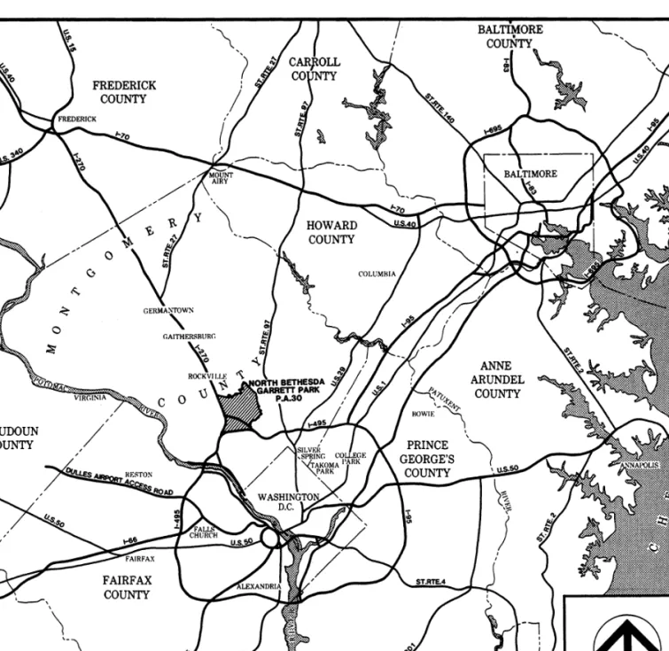
To illustrate with a real example, the north Bethesda, Maryland, window shown in Figure 1 has 20 external stations for a window that is approximately 25 mi2(81 km2). The probability of a work trip (generated in the center of the window) being on any of the external stations is the probability it reached the edge (made a trip of about 2.5 mi) divided by 20. If one assumes the negative exponential dis-tribution, the probability of reaching a distance x is e–Axwhere A is an empirical constant (about 0.10 in Washington, D.C., for work trips). The probability of a work trip being on any given external sta-tion link is therefore e–0.25/20 = 0.039. For a relatively large project generating 1,000 peak-hour work trips, there are 39 cars on the typ-ical boundary link: for an Interstate highway serving 10,000 cars per hour, this is 0.39 percent of total traffic; for an arterial with 2,000 cars per hour, this is about 2 percent of traffic. Because nonwork trips are typically shorter, their likelihood of appearing on any given boundary link is even less.
Levinson and Huang Paper No. 970211 47
The issue of a roadway network change is similar; most changes are felt locally in proportion to the size of the change. The underly-ing principle of assignment is the desire of travelers to take the short-est path (in terms of time). A capacity increase on a congshort-ested link will draw traffic from nearby links more than from those far away as travelers switch routes to equalize times on used routes. The process is limited in spatial extent because of nonzero costs to access either the improved link or its near (but imperfect) substitutes such as parallel links. A larger capacity increase tends to affect a larger area, although the exact scope of the effect depends on the specific network geometry and other conditions.
Furthermore, a transportation network is usually designed with a hierarchical structure in terms of capacity and speed. Drivers are generally expected to use driveways to access streets, streets to access major arterials, and arterials to access freeways. Figure 1 shows a hierarchy of roads in terms of traffic volume in the north Bethesda area. Most through traffic is carried by freeways (I-495 and I-270), and some is carried by the arterials Rockville Pike and Randolph Road. The mostly access and egress traffic on residential streets is kept light by a plethora of turn prohibitions. The hierarchy of the network dictates that the impact area from an improvement be proportional to the class of road. Traffic on local streets is more likely to originate and terminate locally. Therefore, to assess the traffic impact caused by a change to a local road, a smaller window can be selected.
However, when all roads in a given direction are oversaturated, no hierarchy of roads in terms of speed can be maintained. Access costs to alternative routes may be small relative to the total travel costs. Any additional traffic volume from a new development or a small change in a single link can have a ripple effect throughout the whole network. Under this unstable situation no appropriate window size smaller than the regional network can be selected. Under this situation even the results from a regional model need to be carefully interpreted. The practical implication of this extreme situation is that when alternative routes are seriously congested a larger window is needed.
DATA AND GEOGRAPHY
The SLATE model has been applied to several areas of Montgomery County, Maryland. Figure 2 presents a map of the Travel/2 model region (the combined Baltimore, Maryland–Washington, D.C., met-ropolitan area), including Montgomery County and the north Bethesda window examined in more depth. The regional model, Travel/2, provides inputs into the windowed local model, SLATE. Summary statistics for Travel/2 and the SLATE models for Bethesda, north Bethesda, and Germantown west are provided in Table 1.
To avoid confusion, traffic zones from the regional model are called zones, whereas those from the windowed model are called
subzones, each with zone comprising one or more (usually about 30)
subzones with conforming boundaries. Two data sources are used for land use in this analysis. For existing residential land uses on the ground, block-level census data are used. For commercial and future residential land uses, the tax assessor’s file is used. Each census block is treated as a traffic subzone in the study; in some of the study areas, each commercial parcel is a subzone as well. By way of comparison, the analysis of north Bethesda with SLATE uses 798 local subzones and 20 external stations representing the rest of the region, whereas the regional modeling system (Travel/2) uses 19 traffic zones to represent this area and 632 zones to represent the rest of the region.
The links and nodes used in the study area were extracted from the census TIGER files; however, much work was still required to apply network attributes such as travel lanes, capacities, and free-flow speeds to the network. Centroids of subzones were computed by using a GIS, and centroid connectors were created by connecting each centroid with the nearest node automatically, whereas hand cor-rection was used to move centroid connectors off major highways where appropriate. Each signalized intersection and all intersections of smaller streets with arterials are coded and modeled.
MODEL
Although the theory of a SLATE model is similar to that of a regional model, the emphasis of a SLATE model differs. With a more detailed network and zone structure, some features that are not possible for inclusion in a regional model can be included in a SLATE model. For example, SLATE contains detailed trip generation and intersec-tion control models, whereas the advantages of the extra detail would be lost in the aggregation error of the regional model.
The SLATE model system is a combination of several attrib-utes: its relationship with the regional model system, the specific model components, the interaction of those components, and the calibration of the model. Both the regional and windowed models are built on the EMME/2 modeling platform (7), supplemented with additional programs written by the authors.
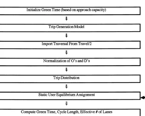
SLATE relies on the regional transportation planning model, Travel/2 (4), which models the afternoon peak hour, to produce sev-eral specific inputs. Ideally, one would have data for more than the afternoon peak hour; however, that is the most congested hour, which places the most stress on the transportation system. The regional model computes the number of trips at stations external to the local window and the distribution pattern of trips between origins and destinations by work and nonwork purpose. The data are tracked by a “traversals” method, which records the number of trips between any marked links. All of the links forming a cordon around the win-dow, as well as all centroid connectors for traffic zones within the window, were marked to obtain a submatrix conforming to the win-dowed model. Furthermore, two classes of trips, work and nonwork, were tracked separately. Any significant changes in the land use or network within the window would be modeled macroscopically in the regional model to update flows at external stations when they may reroute around the area or change entry points within the area. Although the regional model also produces a great deal of other data, that information can be more accurately estimated within the window. SLATE estimates the number of trips by purpose, applies the regional distribution pattern to the specific trip generation in the area to obtain a trip table, assigns the vehicles to the complete road network within the window, and computes intersection delay in equilibrium with the route assignment. The reason for including every roadway in the study window is not to accurately forecast traf-fic on the smaller roads but, rather, to improve traftraf-fic loadings on freeways, highways, arterials, and primary residential streets, as well as to flag potential problems with neighborhood cut-through trips. A simple overview of the model is provided in Figure 3, assuming the presence of input land use data and networks.
Trip Generation and Mode Factors
Because of the land use data available with block- and parcel-level analyses, more than 70 land use activity categories are considered.
Levinson and Huang Paper No. 970211 49
FIGURE 3 Flow chart of SLATE model.
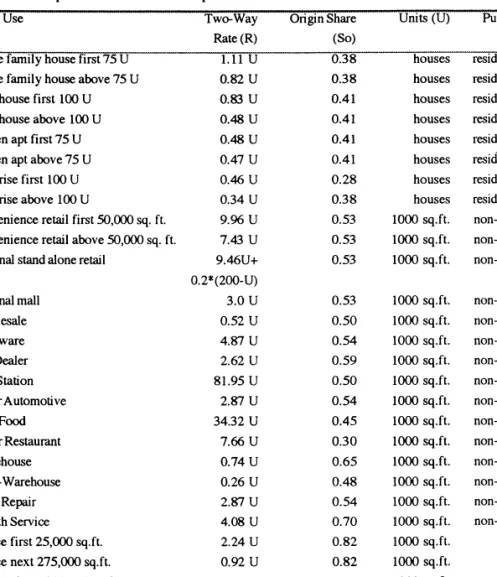
This level of detail is both difficult to achieve in a regional model that relies on multiple jurisdictions for data and not particularly helpful when considering the coarse zone system and networks. Afternoon peak-hour vehicle trip generation rates, presented in Table 2, specific to the land use activity, were derived from local and national studies of major activity classes (residential, office, and large retail) (1,8). The two-way rate (R) multiplied by the origin share (So) gives the number of afternoon peak-hour trip origins;
R multiplied by (1 – So) gives the number of afternoon peak-hour
destinations.
The number of trip origins in regional zone i, subzone s( pis), and
trip destinations from regional zone j, subzone t(qjt), are given by
Equations 1 and 2:
where
R = trip rate,
So = origin share in afternoon peak hour, and
Fx = transit adjustment factors (Fh, Fo, and Fr) for housing,
office, and retail, respectively).
Although the study is dealing with vehicle trips, changes in modal characteristics of transit, ride-sharing, and nonmotorized trans-portation are reflected in several ways. First, vehicle trip rates are discounted on the basis of the distance of the site to the nearest Metro station, of which there are three each in the Bethesda and north Bethesda study areas. The housing vehicle trip adjustment fac-tor (Fh) (Equation 3) is valid for sites within 0.5 mi of a Metro
sta-tion entrance, and reduces trip rates by the distance (D) in feet to the
qjt=R(1−S Fo) x ( )2
pis=R S F( o) x ( )1
nearest Metro entrance. The office vehicle trip adjustment factor (Fo) (Equation 4) is valid within 1,000 ft (1 ft = 0.30 m) of a Metro
station. The retail vehicle trip adjustment factor (Fr) (Equation 5),
applied to sites with more than 300,000 ft2(1 ft2= 0.9 m2) is valid
within 0.25 mi of a Metro station.
In addition, explicit adjustments for travel demand management (TDM) programs are taken into account. These are used to reduce trip rates under a given set of policies. The FHWA TDM model (9) is used for estimation. Any changes in regional mode choice are cap-tured in the regional model, which produces the number of vehicle trips entering and leaving the window at external station. Finally, for any site that satisfied Montgomery County’s transit and pedestrian-oriented neighborhood guidelines (10), its vehicle trip rate was reduced by 5 percent, consistent with the observed data.
Trip Distribution
Trip distribution determines the proportion of trips for which vari-ous destinations are chosen. The choice of destination within the regional model, factored into peak-hour vehicle trips, is solved simultaneously with assignment to ensure consistency between the travel times used to estimate the number of trips and the travel times
Fr = − 0.021,320 −1 D 100 ( )5 Fo= − 0.041, 000 −1 D 100 ( )4 Fh= − 0.02 2,640 −1 D 100 ( )3
TABLE 2 Trip Rates and Directional Splits
resulting from that level of traffic. In the regional model, an equilib-rium assignment model and a multimodal gravity model (11) are used to determine the distribution of trips by mode. The vehicle trip traversal submatrices (work and nonwork) from this equilibrium dis-tribution-assignment are imported into the window. The trip distrib-ution model allocates the number of regional trips between zones by purpose to subzones in proportion to the size of the subzone and by adjustment for under- or overestimation, as discussed in the section Calibration.
A conservation constraint ensures that the total number of trips originating in the window (including external stations) matches the number destined for the window. Normalization is accomplished by splitting the difference between total trip origins and destinations and adjusting the subzone totals accordingly.
′ =
∑
∑
q q p q jt jt is jt 2 1+ ( )7 ′ ∑
∑
p p q p is is jt is = + 2 1 ( )6 Route AssignmentThe highway route assignment is solved by the static user equilib-rium method, which assumes that travelers choose the quickest path. The travel time of each route on the network is composed of link travel time and intersection delay. The general form of the link delay functions was developed previously (12) and is described in Equation 8. Model coefficients are given in Table 3.
T T A Q Q B Q Q f o o c c = 1+ exp + ( )8
Levinson and Huang Paper No. 970211 51
where
Tc = congested travel time,
Tf = free-flow travel time,
Q = flow (in vehicles per hour per lane), Qo = capacity (in vehicles per hour per lane), and
A, B, c = estimated parameters.
Intersection Control
Most transportation planning models either ignore traffic signal tim-ing or consider it exogenous to the model system, and thus inde-pendent of route assignment. This presumption of independence is counter intuitive and is more a result of modeling difficulties [such as level of details of the model and difficulties in modeling the non-convex traffic assignment (13)] than any theory. Empirical evidence (14), however, suggests that signal delay, including both stopped and approach delay, amounts to more than 29 percent of total delay time on arterials in Montgomery County and the vast majority of all delay. Furthermore, the level of detail of a SLATE model enables proper modeling of intersection delay for planning purposes. Expe-rience also indicates that the nonconvexity of intersection delay, off-set by the strong convexity of link delay, does not cause serious convergence problems for the model.
Several attempts have been made to integrate an assignment algorithm with intersection control (15–17) in more or less realis-tic systems. The nature of combining the two systems is such that initial assumptions and the equilibration algorithm can influence final outcome. Because the SLATE model aims to reproduce real-istic flows rather than optimize signal settings, it was decided that assumptions that seemed realistic, instead of spending considerable effort searching for optimal settings, would be taken. It should also be noted that an isolated intersection model is used for conve-nience, although it is known that signal settings are coordinated in the windowed model areas.
The output of the intersection control model is the green time, cycle length, and effective number of turning lanes (when lanes are shared) for a turning movement. The cycle time and green time are estimated by methods suggested previously (18), whereas lane adjust-ment factors and lane utilization factors are adopted from Chapter 9 of the Highway Capacity Manual (19). The green time is assigned to equalize the volume/saturation flow on the critical approaches.
where
C = cycle length (sec), L = lost time per cycle (sec),
Q = flow on movement in vehicles per study period (T), Qo = saturation flow rate (1,800 vehicles per hour of green), and
p = phase.
This in turn is imported into the assignment model, in which a turn penalty function estimates the delay model on the basis of the following model (20): d C g C Q Q g C o = − +2 − 2 1 1 10 T ( ) C L Q Qo p = + − = 1 5 5 1 0 9 1 4 . . ( )
∑
whered = average delay (sec),
T = length of congested time period (sec), and g = green phase length (sec).
To ensure stability and more rapid convergence, an equilibration algorithm is used. On the initial iteration, before link volumes are known, the green time (go) is allocated on the basis of approach capacities, with the approaches with the most capacity being given the most green time. On subsequent iterations the green time (gi) is
calculated by using the volumes from the previous iteration in a manner that would equalize the volume-to-capacity ratios for the critical movements at each approach by assuming a four-phase intersection (or three phases for a T-intersection). Excess time from the noncritical left-turn movements are given to the complementary through movement.
On the subsequent iterations, however, to ensure convergence, an accumulating average is used to estimate the green time actually input into the model for the next iteration of assignment. This value is the adjusted green time (g′i), which is computed by using the
following equation:
CALIBRATION
Despite the best efforts to capture detail in the model specification, no model will be able to include all variables in the real world or will have perfectly accurate data for the variables included in the model. Thus, model calibration is needed. The calibration was conducted in several stages, principally to account for the missing variables by matching base year (1990) modeled link flows and on-ground traf-fic counts. This is done both by adjusting the number of trips enter-ing the window and the number of trips between zones and by correcting any errors remaining on specific links and turning move-ments. The first two model calibration methods are internal to the model, and the last is a postprocessor.
A general issue surrounding model calibration is how to adjust the model estimates to match the observed values. Two approaches come immediately to mind; adding the difference (observed value – estimated value in the base year) to the forecast estimate, assum-ing that traffic induced by the missassum-ing variables will change in the future, or multiplying the forecast estimate by the ratio of the observed value to the estimated value in the base year, assuming that the traffic induced by the missing variables will change pro-portionally to the traffic induced by other variables (or, if it is not strictly proportional, the ratio still provides a first-order approxi-mation of many functional forms). Because the nature of these missing variables is not known a priori (if they were known the problem would have been corrected elsewhere), then one needs to make an educated judgment. It is important to recognize that there is no guarantee that these adjustment factors remain stable over time, but making such adjustments is almost surely better than not making them. The approach taken here is to combine the two methods: ′
[
]
X WX X X W X X X Q e o e = + −(1 ) +( − ) (12) ′ ′( ) ( )
g i g i i g i i i = −1 − + 1 1 11 ( )where
X′ = adjusted forecast estimate,
X = unadjusted forecast estimate, Xo = base year observation,
Xe = base year unadjusted estimate, and
W = weight to combine methods (between 0 and 1; here it is
assumed that W is equal to 0.5).
First, the number of trips entering or leaving the window at exter-nal stations was adjusted according to Equation 12. This corrects for any under- or overestimation from the regional model. Cordon counts from several sources were used to provide a base year observed value. Second, a gradient adjustment method (21) was applied to adjust the window’s modeled base year vehicle trip table to minimize the dif-ference between modeled and observed traffic counts on links within the window. The gradient adjustment method ensures that the cells of the trip table that have the most impact on imbalance between esti-mated and actual traffic counts are adjusted most. Running the gradi-ent adjustmgradi-ent algorithm for 10 iterations in the Bethesda window cut the error by two-thirds. The r2value (estimated traffic count regressed on observed traffic count) increased from 0.77 before calibration to 0.90 after iteration 10. The entire trip table was reduced from 58,500 to 54,300 trips. For the base year this returns the improved trip table, and for future year it provides a more probable estimate.
Third, as a postprocessor, turning movements at individual inter-sections from the model were adjusted to match turning movement counts. The adjusted turning movement counts were used to calcu-late critical lane volumes and other level-of-service indicators used to recommend policy. This process may not increase the prediction power of the model, but it does provide consistent estimates for policy purposes.
The accuracy of the SLATE model can be compared with that of the regional model, because the primary reason for using a window is improved accuracy. In the case of north Bethesda for the same base year (1990), after adjusting the trip tables but before using any postprocessors, the r2value (estimated traffic count regressed on observed traffic count) from the SLATE model was 0.95 on 496 links with observations, whereas for the regional model, the r2value was 0.67 on 79 links with observations.
CONVERGENCE
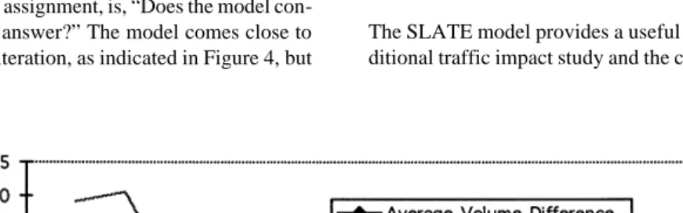
A key question to ask of the model, particularly because it integrates intersection control with route assignment, is, “Does the model con-verge to a single equilibrium answer?” The model comes close to its final answer after the fifth iteration, as indicated in Figure 4, but
because this paper is dealing with a nonconvex problem combining signal timing and route assignment, each with different objective functions and solution methods, there is no reason to expect a final true equilibrium answer. This disequilibrium is despite the equili-bration algorithm used in the intersection control module. In fact, even at iteration 15 there are small fluctuations (plus or minus three vehicles per hour on the average link) of volume (flow) on links from iteration to iteration, although fluctuations tend to get smaller iteration after iteration. For this reason interpretation of the model for comparison of alternatives should be looking at differences larger than this to ensure that they are significant. Because the aver-age volume difference is usually positive, this indicates that most links are gaining volume from iteration to iteration. This is also to be expected: on the first iteration, all cars are assigned to the shortest path (in terms of free-flow time); but after they all take this path, it is no longer the shortest path. On subsequent iterations the equilibrium assignment moves vehicles to less congested routes. Because there are more routes that are not the shortest path than there are routes that are the shortest path, most routes gain volume as the traffic is spread over the network.
APPLICATION
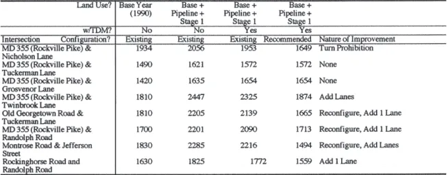
The SLATE model has been applied in several areas of Montgomery County: Germantown west, Bethesda, north Bethesda, Rockville, and Glenmont. The principal intention of these applications was to conduct a comprehensive local-area transportation review, which would supplant developer-funded traffic impact studies in these areas. All of the areas are nodes of growth designated by the county’s master plans, and most are centered on Metro stations. The modeling analysis was coupled with various policy changes, urban design recommendations, and incentives and requirements for use of travel modes other than the single-occupant vehicle. To illustrate the use of the model for linking transportation and growth manage-ment, the case of north Bethesda (illustrated in Figure 1) is exam-ined. Table 4 summarizes the results of a level-of-service analysis with SLATE in north Bethesda, testing changes in land use, travel demand management policies, and network configuration. The mod-eling analysis recommended a number of intersection improvements that were adopted as part of the area master plan (22).
CONCLUSIONS
The SLATE model provides a useful tool situated between the tra-ditional traffic impact study and the comprehensive regional travel
Levinson and Huang Paper No. 970211 53
TABLE 4 Summary of Intersection Level of Service, North Bethesda SLATE
demand analysis. By combining computerization, which enables the flexible estimations of impacts of alternative scenarios while considering regional demand impacts, with the detail of including every street and assigning a traffic zone to each parcel, the microscale planning needed for studying intersections in tightly packed urban areas can be conducted. Traffic impact studies that do not consider how new developments cause existing traffic to reroute miss a significant factor that is easily captured in this modeling framework.
This model indicates the sensitivity of traffic patterns to inter-section control. Also worth noting are the air quality impacts of stopped delay and running speed. Given current fuel choices by the vehicle fleet and present technologies, valid estimates of air pollu-tion need to be able to determine stopped delay, running speed, and total traffic demand. Incorporating the intersection in the planning model is necessary for proper implementation of Clean Air Act requirements.
Although the model is useful, it can always be improved. A key theoretical weakness is the assumption of isolated intersection control. A more rigorous approach would optimize signals on a sys-temwide basis, such as with TRANSYT, or on an arterial basis, such as with MAXBAND. Integration with a local-area network simula-tion, such as NETSIM, may also provide more accurate intersection flows. However, this will push the model to another level of detail requiring inputs of much traffic operation data not available at the planning stage, although SLATE is intended for subarea planning purposes.
Another possible improvement is to close the information feed-back loop by taking results from a window and reintegrating them with the regional model (23). These can include results for model calibration as well as forecast application. The loop will either increase the accuracy of the windowed model or reduce the size of window needed, or both. In addition, further research on the size of the window and the accuracy of the model under different network architectures, traffic conditions, and land uses is needed. This will give more guidance for planners using windowed models.
ACKNOWLEDGMENTS
The authors acknowledge Ajay Kumar, Bud Liem, Bob Winick, Michael Replogle, John Bailey, Don Vary, and Sara Loftus, for-merly of the Montgomery County Planning Department, as well as current staff, in particular Ed Axler, Yetta McDaniel, Ivy Leung, Eric Graye, and Richard Hawthorne.
REFERENCES
1. Local Area Transportation Review Guidelines. Montgomery County Planning Board, Silver Spring, Md., 1996.
2. Traffic Impact Analysis. APA Planning Advisory Service 384. American Planning Association, Chicago, 1984.
3. Boyce, D. E., L. LeBlanc, and K. Chon. Network Equilibrium Models of Urban Location and Travel Choices: A Retrospective Survey. Journal of
Regional Science, Vol. 28, No. 2, 1988.
4. Levinson, D., and A. Kumar. Integrating Feedback into the Transporta-tion Planning Model: Structure and ApplicaTransporta-tion. In TransportaTransporta-tion
Research Record 1413, TRB, National Research Council, Washington,
D.C., 1994.
5. Horowitz, A. J. Implementing Travel Forecasting with Traffic Opera-tional Strategies. In Transportation Research Record 1365, TRB, National Research Council Washington, D.C., 1992.
6. FY95 Annual Growth Policy. Montgomery County Planning Department, Silver Spring, Md., 1994.
7. EMME/2 User’s Manual: Release 6. INRO, Montreal, Quebec, Canada, 1993.
8. Trip Generation, 5thed. ITE, Washington, D.C., 1990.
9. Comsis Corp. Transportation Demand Management Computer Model. FHWA, U.S. Department of Transportation, 1993.
10. Transit Pedestrian Oriented Neighborhoods: Design Study. Montgomery County Planning Department, Silver Spring, Md., 1993.
11. Levinson, D., and A. Kumar. A Multimodal Trip Distribution Model: Structure and Application. In Transportation Research Record 1466, TRB, National Research Council, Washington, D.C., 1995, pp. 124–131. 12. Travel/2 A Simultaneous Approach to Transportation Planning. Montgomery County Planning Department, Silver Spring, Md., 1991. 13. Newell, G. Non-Convex Traffic Assignment on a Rectangular Grid Net-work. Research Report UCB-ITS-RR-94-7. Institute of Transportation Studies, University of California at Berkeley, 1994.
14. Levinson, D. Speed Flow and Density on Signalized Arterials. Working paper. 1995.
15. Charlesworth, J. A. The Calculation of Mutually Consistent Signal
Set-tings and Traffic Assignment for a Signal-Controlled Road Network.
Transport Operations Research Group, University of Newcastle upon Tyne, United Kingdom, 1977.
16. Van Vuren, T., M. J. Smith, and D. Van Vliet. The Interaction Between Signal Setting Optimization and Reassignment: Background and Pre-liminary Results. In Transportation Research Record 1142, TRB, National Research Council, Washington, D.C., 1988.
17. Tan H., S. Gershwin, and M. Athans. Hybrid Optimization in Urban
Traffic Networks. FHWA Report DOT-TSC-RSPA-79-7. FHWA, U.S.
Department of Transportation, 1979.
18. McShane, W., and R. Roess. Traffic Engineering. Prentice-Hall, Englewood Cliffs, N.J., 1990.
19. Special Report 209: Highway Capacity Manual. TRB, National Research Council, Washington, D.C., 1985.
20. Hurdle, V. Signalized Intersection Delay Models: A Primer for the Uninitiated. In Transportation Research Record 971, TRB, National Research Council, Washington, D.C., 1984.
21. Spiess, H. A Gradient Approach for the O-D Matrix Adjustment Problem. Center for Transportation Research Paper 692. Center for Transportation Research, University of Montreal, Quebec, Canada, 1990.
22. North Bethesda–Garrett Park Master Plan Staging Amendment to the
1992 Master Plan. Montgomery County Planning Department, Silver
Spring, Md., 1993.
23. Winslow, K. B., K. Bladikas, K. J. Hausman, and L. N. Spasovic. Intro-duction of Information Feedback Loop To Enhance Urban Transporta-tion Modeling System. In TransportaTransporta-tion Research Record 1493, TRB, National Research Council, Washington, D.C., 1996, pp. 81–89.
Publication of this paper sponsored by Committee on Passenger Travel Demand Forecasting.