Final degree work
COMPUTER ENGINEERING DEGREE
Faculty of Mathematics
University of Barcelona
CAROTID ARTERY IMAGE
SEGMENTATION
Author: Laia Nadal Zaragoza
Director:
Laura Igual Mu˜
noz
Made in:
Department of Applied
Mathematics and Analysis
Abstract
The main process causing most cardiovascular diseases is atherosclerosis, which is responsible for the thickening of the major arteries walls. Concretely, the intima-media thickness (IMT) of the carotid artery wall is an early and effective marker of atherosclerosis progression. The measurement of the IMT is directly extracted from the segmentation of two different layers of the carotid artery wall. In this project, we present three fully automated techniques to perform the segmentation of these two layers of the carotid artery wall using B-mode ultrasound images. The segmentation of the carotid artery wall is a challenging problem due to image noise, artifacts and image shape, intensity and resolution variability. One of the developed methods is based on lumen detection. It first detects the lumen region of the carotid artery and then it seeks the both layers using the differences between the intensity values of the image. The other two methods are based on a classification system, considering the image segmentation problem as a classification problem of the image pixels into interior or exterior of the region formed by the two layers. One of them uses the random forest classifier and the other one uses the stacked sequential learning scheme with random forest as a base learner. We validate the proposed techniques using a data set of B-mode images obtained from a clinical institution and we compare its performances.
Resum
El principal proc´es que causa la gran majoria de les malalties cardiovasculars ´es l’aterosclerosi, que comporta un engruiximent de la paret de les art`eries m´es im-portants. Concretament, el gruix de la regi´o intima-media de la paret de l’art`eria car`otida, anomenat IMT en l’`ambit cl´ınic, ´es un indicador efectiu de la progressi´o de l’aterosclerosi. El mesurament de l’IMT s’extreu directament de la segmentaci´o de dues capes de la paret de la car`otida. En aquest projecte, presentem tres t`ecniques completament autom`atiques per segmentar aquestes dues capes de la paret de l’art`eria car`otida utilitzant imatges d’ultras`o. La segmentaci´o de la paret de la car`otida suposa un problema dif´ıcil degut al soroll de les imatges, artefactes i variabilitat en la forma, intensitat i resoluci´o de les imatges. Un dels m`etodes desenvolupats es basa en la detecci´o de la regi´o del flux sanguini (lumen). Primer es detecta aquesta regi´o i despr´es es busquen les dues capes utilitzant les difer`encies entre els valors d’intensitat de la imatge. Els altres dos m`etodes es basen en un sistema de classificaci´o, considerant el problema de segmentaci´o de la imatge com un problema de classificaci´o dels seus p´ıxels en interior o exterior de la regi´o form-ada per les dues capes. Un d’ells utilitza el classificador anomenatrandom forest i l’altre utilitza l’esquema anomenat stacked sequential learning amb random forest
com a classificador base. Les tres t`ecniques proposades s´on validades utilitzant un conjunt d’imatges d’ultras`o obtingudes d’una instituci´o cl´ınica i es comparen els resultats obtinguts.
Resumen
El principal proceso que causa la gran mayor´ıa de las enfermedades cardiovasculares es la aterosclerosis, que conlleva un engrosamiento de la pared de las arterias m´as importantes. Concretamente, el grosor de la regi´onintima-media de la pared de la arteria car´otida, llamado IMT en el ´ambito cl´ınico, es un indicador efectivo de la progresi´on de la aterosclerosis. La medici´on del IMT se extrae directamente de la segmentaci´on de dos capas de la pared de la car´otida. En este proyecto, presentamos tres t´ecnicas completamente autom´aticas para segmentar estas dos capas de la pared de la arteria car´otida utilizando im´agenes de ultrasonido. La segmentaci´on de la pared de la car´otida supone un problema dif´ıcil debido al ruido de las im´agenes, artefactos y variabilidad en la forma, intensidad y resoluci´on de las im´agenes. Uno de los m´etodos desarrollados se basa en la detecci´on de la regi´on del flujo sangu´ıneo (lumen). Primero se detecta esta regi´on y luego se buscan las dos capas utilizando las diferencias entre los valores de intensidad de la imagen. Los otros dos m´etodos se basan en un sistema de clasificaci´on, considerando el problema de segmentaci´on de la imagen como un problema de clasificaci´on de sus p´ıxeles en interior o exterior de la regi´on formada por las dos capas. Uno de ellos utiliza el clasificador llamado
random forest y el otro utiliza el esquema llamado stacked sequential learning con
random forest como clasificador base. Las tres t´ecnicas propuestas son validadas utilizando un conjunto de im´agenes de ultrasonido obtenidas de una instituci´on cl´ınica y se comparan los resultados obtenidos.
Acknowledgements
To my director Laura Igual for her excellent work, the knowledge, assistance and support she has given me as well as her confidence and patience during the entire project. I really enjoyed working with her.
To Maria del Mar Vila for the great help she has provided me when I have needed it.
To my family, who has given me the opportunity to study this degree, for their unconditional and continuous support. Without them the project would not have been possible.
To my friends and colleagues for the motivation they have given me during all the degree.
Contents
1 Introduction 1
1.1 Background of the clinic problem . . . 1
1.2 Carotid artery and IMT measurement . . . 2
1.3 Motivation and objectives of the project . . . 4
1.4 Document structure . . . 6 2 Planning 7 2.1 Initial planning . . . 7 2.2 Real planning . . . 8 2.3 Economic evaluation . . . 8 3 Related work 10 4 Methodology 13 4.1 Supervised classification system . . . 13
4.2 Random forest . . . 14
4.3 Stacked sequential learning . . . 15
5 Development 19 5.1 LI-MA segmentation based on lumen extraction . . . 19
5.2 LI-MA segmentation based on a classification system . . . 21
5.2.1 Feature extraction . . . 22
5.2.2 Pre-processing step . . . 27
5.2.3 Classification system: training stage . . . 27
5.2.4 Classification system: test stage . . . 29
5.2.5 Post-processing step . . . 30 5.3 Programming language . . . 32 6 Experimental results 33 6.1 Data set . . . 33 6.2 Validation measures . . . 33 6.3 Results . . . 34 6.3.1 Quantitative results . . . 34
6.4 Execution time . . . 46
7 Conclusions 47
List of Figures
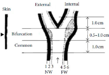
1 (a) Course of the carotid artery along the neck. (b) Anatomy of the
different carotid artery vessels.1 . . . 3
2 Drawing of the carotid artery with the boundaries: (1) adventi-tia (NW), (2) adventiadventi-tia-media (NW), (3) intima-lumen (NW), (4) lumen-initima (FW), (5) media-adventitia(FW) and (6) adventitia (FW). NW = Near Wall. FW = Far Wall. Image obtained from [19]. 3 3 Ultrasound longitudinal image of the CCA. The picture indicates the near wall, the far wall, the lumen (L), the LI and MA boundaries and the IMT. Image obtained from [9]. . . 4
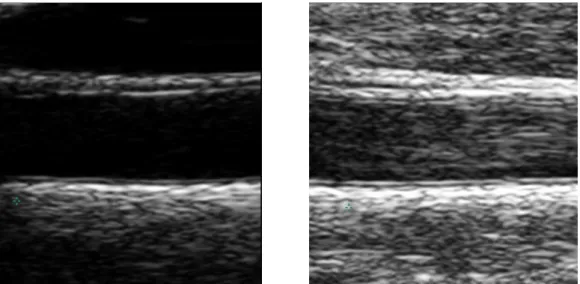
4 (a) Ultrasound longitudinal image of the CCA with plaque (green lines). (b) Ultrasound longitudinal image of the CCA without plaque (green lines). . . 5
5 Two different ultrasound longitudinal images of the CCA with dif-ferent intensities. . . 6
6 Gantt diagram of the initial planning. . . 7
7 Gantt diagram of the real planning. . . 8
8 Supervised classification scheme. . . 13
9 Binary decision tree with its node functionstp < λp defined by CART algorithm. Image obtained from [14]. . . 15
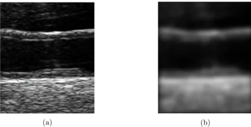
10 Stacked sequential learning scheme, W=2. Image obtained from [4]. 17 11 Example of an image after applying the Gaussian smoothing filter. (a) Original image. (b) Smoothed image. . . 20
12 Example of the output of the lumen detection. (a) Original im-age. (b) The red region indicates the detected lumen region by the method. (c) The yellow line indicates the bottom boundary of the detected lumen and the blue line indicates the considered bottom lumen boundary after moving it upwards. . . 20
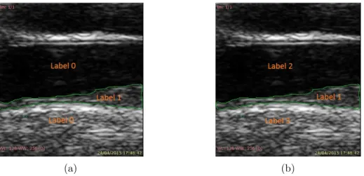
13 Labels assignment. Green lines indicate the LI-MA region. (a) Case of two labels. (b) Case of three labels. . . 22
14 General flowchart of the methods based on a classification system. . 22
15 Illustration of the patch definition. . . 22 16 Plot of the mean and the standard deviation of the data values for
each feature separated by labels. The means correspond to the graph-ics drawn and the standard deviations are the horizontal lines. The x axis is the features (predictors) and the y axis is the intensity values.
Graphic in the case of two labels. Blue corresponds to label 1 and pink corresponds to label 0. The blue lines overlap part of the
17 Plot of the mean and the standard deviation of the data values for each feature separated by labels. The means correspond to the graph-ics drawn and the standard deviations are the horizontal lines. The x axis is the features (predictors) and the y axis is the intensity val-ues. Graphic in the case of three labels. Blue corresponds to label 1, red corresponds to label 2 and green corresponds to label 3. The green lines overlap part of the blue lines because they are drawn above them. . . 24 18 Histograms in the case of two labels. Blue corresponds to label 1 and
pink corresponds to label 0. The x axis is the intensity values and the y axis is the number of cases belonging to the bins. (a) Histogram of the intensity values of each example that belongs to label 1. (b) Histogram of the intensity values of each example that belongs to label 0. . . 25 19 Histograms in the case of three labels. Blue corresponds to label 1,
red corresponds to label 2 and green corresponds to label 3. The x axis is the intensity values and the y axis is the number of cases belonging to the bins. (a) Histogram of the intensity values of each example that belongs to label 1. (b) Histogram of the intensity values of each example that belongs to label 2. (c) Histogram of the intensity values of each example that belongs to label 3. . . 26 20 Example of the definition of the ROIs in the training stage. (a) Image
of the first training ROI explained in the text. Green corresponds to GT, blue corresponds to the ROI obtained and the red points represent the lower and the higher rows of the GT, which are used as a reference to build the rectangle. The vertical distance between the red point and the rectangle is θ1. (b) Image of the the second
training ROI explained in the text. Green corresponds to GT, blue corresponds to the ROI obtained. The vertical distance between blue and green lines (top and bottom) for each column of the image is θ2. 28
21 Example of the definition of the ROIs in the test stage. (a) Train-ing image used to construct the first test ROI explained in the text. (b) Training image used to construct the second test ROI explained in the text. In both cases, blue corresponds to a ROI obtained in the training stage, red corresponds to the lumen detection output, the yellow point R represent the point selected of the bottom lu-men boundary used as a reference to compute the differences up and differences down, differences up = R-A and differences down = B-R. 30 22 Post-processing example. (a) Mask with the classification result for
the label 1 (without post-processing). (b) Fill holes step output. (c) Opening operation output. (d) Closing operation output. (e) Final output of the post-processing step. . . 31 23 Example of a mask with the classification result with its ROI painted
24 Qualitative results of the method based on lumen detection. Green corresponds to the GT, blue corresponds to the segmentation obtained for LI and red corresponds to the segmentation obtained for MA. . . 39 25 Qualitative results of random forestusing training ROI 1and test
ROI 1 in the case of two labels. Green corresponds to the GT and blue corresponds to the segmentation obtained for the LI-MA region. 40 26 Qualitative results of random forestusing training ROI 1and test
ROI 1 in the case of three labels. Green corresponds to the GT and blue corresponds to the segmentation obtained for the LI-MA region. . . 41 27 Qualitative results of stacked sequential learning in the case of
two labels. Green corresponds to the GT and blue corresponds to the segmentation obtained for the LI-MA region. . . 42 28 Qualitative results of stacked sequential learning in the case of
three labels. Green corresponds to the GT and blue corresponds to the segmentation obtained for the LI-MA region. . . 43 29 Qualitative results of random forestusing training ROI 2and test
ROI 2 in the case of two labels. Green corresponds to the GT and blue corresponds to the segmentation obtained for the LI-MA region. 44 30 Two example images to comparestacked sequential learning and
multi-scale stacked sequential learning. For each image, the first row corresponds to stacked sequential learning and the second row corresponds to multi-scale stacked sequential learning; the first column corresponds to output of the first step of stacked sequen-tial learning scheme, the second columns corresponds to the output without post-processing step and the third column corresponds to the output with post-processing step. Green corresponds to the GT and blue corresponds to the segmentation obtained for the LI-MA region. . . 45
List of Tables
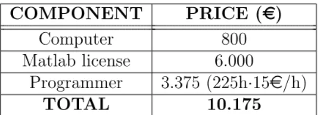
1 Tasks and estimated duration for the initial planning. . . 7 2 Tasks and estimated duration for the real planning. . . 8 3 Prices of all the components required for the project. . . 9 4 Percentage of each label in the training data S depending on the ROI
used. Case of two labels. ROI 1 refers to the first ROI explained in section 5.2.3 and ROI 2 refers to the second one. . . 28 5 Percentage of each label in the training data S depending on the ROI
used. Case of three labels. ROI 1 refers to the first ROI explained in section 5.2.3 and ROI 2 refers to the second one. . . 28 6 Quantitative results of the overlap and the distance function for the
method based on lumen detection. . . 34 7 Quantitative results for the methods based on a classification system
using all the images for the validation. RF=Random Forest, SSL=Stacked Sequential Learning, MSSL=Multi-scale Stacked Se-quential Learning, without post-process means without applying the processing step, with post process means applying the post-processing, Acc=Accuracy, Sens=Sensitivity, Spec=Specificity and Ov=Overlap. For the training ROIs, ROI 1/ROI 2 refers to the first/second ROIs explained in section 5.2.3. For the test ROIs, ROI 1/ROI 2/ROI 3 refers to the first/second/third ROIs explained in section 5.2.4. Bold rows indicate the best result for RF and for SSL. 36 8 Quantitative results for the methods based on a classification
sys-tem using the images with low IMT and the images with high IMT separately for the validation. RF=Random Forest, SSL=Stacked Sequential Learning, Acc=Accuracy, Sens=Sensitivity, Spec=Specificity and Ov=Overlap. The training ROI 1 refers to the first ROI explained in section 5.2.3. The test ROI 1 refers to the first ROI explained in section 5.2.4. Bold rows indicate the best result for RF and for SSL. . . 37 9 Execution times for each method developed. For the training ROIs,
ROI 1/ROI 2 refers to the first/second ROIs explained in section
5.2.3. For the test ROIs, ROI 1/ROI 2/ROI 3 refers to the first/second/third ROIs explained in section 5.2.4. . . 46
1
Introduction
The framework of this work is a research project developed in PRBB2 by a team of
professors of the Mathematics Faculty of the University of Barcelona together with the clinical institution REGICOR3. This research project deals with the clinical
problem introduced below.
In this section we introduce, as said before, the clinical problem of this work followed by some anatomical details and clinical measures. The motivation and technical objectives of the work are also introduced.
1.1
Background of the clinic problem
The number one cause of death is cardiovascular diseases (CVDs), representing 31% of all global deaths in 2012 according to World Health Organization [11]. CVDs are disorders of the heart and blood vessels. The CVDs that are responsible for most deaths are heart attacks and strokes. The leading cause of heart attacks and strokes is atherosclerosis, a condition that provokes a thickening of the artery walls due to plaque formation. This plaque is mainly made of lipids and blocks the blood’s flow. Atherosclerosis starts early in life and becomes dangerous with aging. This condition usually does not cause symptoms until it is severely advanced, so the key to decrease the number of deaths due to CVDs is prevention.
The most used marker for early stages of atherosclerosis and cardiovascular risk is the increase in carotid artery intima-media thickness (IMT). Therefore, the meas-urement of IMT for the assessment of the artery is of paramount importance for the prevention of CVDs.
Ultrasound images of carotid artery are the most used tool for diagnosis of carotid plaques. They allow the assessment of the artery and the measurement of the IMT to evaluate the progression of atherosclerosis. Ultrasound technique has the advant-ages of being non-invasive, safe for the patients because it does not use dangerous radiations, real-time, reliable and the equipment is economic. The main drawbacks of this methodology are that ultrasounds are operator dependent, causing variations in ultrasound images of the same location obtained by different operators; and that ultrasound images have a low signal-to-noise ratio that reduces the quality of the images.
1.2
Carotid artery and IMT measurement
The carotid artery [20] is a major blood vessel that ascends in the neck in order to supply blood to the brain, neck and face. We have two carotid arteries, one on the left side and one on the right side. Figure 1(a) shows the situation of the carotid artery.
The carotid artery is divided into three vessels: the common carotid artery (CCA), the external carotid artery (ECA) and the internal carotid artery (ICA). The CCA is the main vessel and bifurcates into two branches: the ICA, which supplies blood to the brain; and the ECA, which supplies blood to the neck and face. This bifurcation is called carotid bulb and it is characterized by an enlargement of the vessel. The differentiation of the ICA and ECA is based on their depth from neck skin. Figure 1(b) shows the anatomy of the carotid artery.
The carotid artery walls are made of three layers: adventitia, the outer layer; media, the middle layer; and intima; the inner layer. The transition from the lumen (blood) to the intima layer is called lumen-intima (LI), and the transition from the media layer to the adventitia layer is called media-adventitia (MA). The walls are called near wall and far wall also depending on their depth from neck skin. The distinct layers of the carotid artery are shown in Figure 2.
The IMT is defined as the distance between the LI and MA interfaces. See Figure 3 for an example. The IMT can be visualized in a longitudinal image of any carotid artery part (ECA, ICA, CCA, bulb) on both walls of the vessel. However, the distinction between the different layers is more obvious in the far wall than in the near wall and, for this reason, is more common to measure the IMT of the carotid artery far wall. In addition, the amount of plaque is higher in the ICA and the bulb, but it is hard to distinguish the LI and MA boundaries there because of the low image quality in these zones. So the IMT is generally measured in the CCA.
In order to assess the IMT and determine if it can be considered as plaque, the Mannheim consensus is applied [17]. According to the Mannheim consensus, plaque is defined as a focal structure that encroaches into the arterial lumen of at least 0.5mm or 50% of the surrounding IMT value or demonstrates a thickness higher than 1.5mm. So if the measured IMT is lower than 1.5mm, it is said that the carotid artery has no plaque and has low IMT; otherwise it is said that the carotid artery has plaque and has high IMT.
(a) (b)
Figure 1: (a) Course of the carotid artery along the neck. (b) Anatomy of the different carotid artery vessels.4
Figure 2: Drawing of the carotid artery with the boundaries: (1) adventitia (NW), (2) adventitia-media (NW), (3) intima-lumen (NW), (4) lumen-initima (FW), (5) media-adventitia(FW) and (6) adventitia (FW). NW = Near Wall. FW = Far Wall. Image obtained from [19].
Figure 3: Ultrasound longitudinal image of the CCA. The picture indicates the near wall, the far wall, the lumen (L), the LI and MA boundaries and the IMT. Image obtained from [9].
1.3
Motivation and objectives of the project
As said in the previous section, measurement of the IMT using ultrasound images of the CCA is the most widely used clinical exam for the evaluation of the progression of atherosclerosis.
Habitually, the IMT is manually measured by a trained operator directly from the ultrasound image during the exam, by drawing two markers on the image. Nevertheless, manual measurements are user dependent, time consuming, prone to errors and nonviable when a large number of images should be analyzed.
As the IMT is the distance between the LI and MA interfaces, its measurement is related to the segmentation of the CCA wall. Segmentation of the CCA wall means tracing the LI and MA boundaries (see Figure 3). The aim of performing the segmentation of the CCA wall is to measure the IMT using the segmentation acquired, so it is a previous step for the IMT measurement.
In order to avoid the manual measurement of the IMT and the manual segment-ation of the CCA wall, many computer applicsegment-ations for the IMT measurement and the segmentation of the CCA wall have been developed. These techniques can be di-vided into semi-automated and completely automated. A semi-automated method needs some user interaction whereas a completely automated method does not need any user interaction during its execution.
The purpose of this work is to carry out a research project to develop a fully automated technique to perform the segmentation of the CCA far wall using ultra-sound B-mode longitudinal images5. Therefore, the project consists in developing
5See section 6.1 to know the source of the ultrasound images we have to develop the project.
a method that automatically traces the LI and MA boundaries of the far wall of the CCA.
The difficulties of the segmentation come from the different appearances of the LI and MA interfaces in the images and the fact that the images are a type of ultrasound imaging. The first one is due to the fact that the LI and MA boundaries morphology changes depending on whether the CCA of the image has plaque (high IMT) or not (low IMT). Figure 4 shows an example of a CCA with plaque and another example of a CCA without plaque in order to appreciate the difference in the appearance of the LI-MA region which is marked in green. The second diffi-culty concerns that the ultrasound has particular characteristics that complicate the segmentation problem. One characteristic is the noise of the image. It can be caused by the sound waves, that reduces the quality of the images; or by artifacts such as aggregated red cells, which causes that artery lumen appears brighter than it should be; and calcium deposition, causing shadowing on the ultrasound image. Another ultrasound characteristic is that the resolution of the images is different depending on the source. Finally, another characteristic is the intensity variability of the images that provokes having very bright images while others very dark. See Figure 5 for an example of intensity variability.
(a) (b)
Figure 4: (a) Ultrasound longitudinal image of the CCA with plaque (green lines). (b) Ultrasound longitudinal image of the CCA without plaque (green lines).
Figure 5: Two different ultrasound longitudinal images of the CCA with different intensities.
1.4
Document structure
The document is structured as follows. Section 2 reports how the whole project was planned initially, how the project was really planned after its development and an economic estimation for the project. Section 3 summarizes several papers related to the problem treated in this work. Section 4 reviews the methods used for the project development. Section 5 explains the different implemented algorithms carried out during the project to reach the objectives. Section 6 introduces the data set used, explains the different validation measures computed to evaluate the algorithms, shows the quantitative and qualitative results obtained, presents a discussion on the results and shows the execution time of the methods. Section 7 covers the conclusions and future work.
2
Planning
This section shows the planning of the project before starting it and the real plan-ning after finishing it. Then, the economic cost that would have the project is estimated.
2.1
Initial planning
Before starting the project, a previous planning of the project timeline was done. This planning consists in predicting the tasks that should be done to develop the project and estimating the time required for each task.
The main tasks considered to make the planning are: preparation, development and memory writing. The preparation is the first step and consists in reading different papers in order to get knowledge about the subject. This task also includes getting familiar with the programming language and its tools. The following task is development. This task can be divided into implementation and testing and results. The implementation includes the code development and the testing and results consist in doing different tests and validate them. The last task is the memory writing to explain all the development of the project.
The final degree work consists of 18 ECTS credits and each credit corresponds to 25 work hours. So, the final degree work is equivalent to 450 work hours. In order to develop the project, the number of available weeks is 20. Then, the amount of hours of work during a week is 22.5. With this in mind, the estimated time for each task is written in Table 1. Figure 6 shows the Gantt diagram of the initial planning.
TASKS ESTIMATED DURATION (Weeks)
Preparation 5
Project development 10
Implementation 6
Testing and results 4
Memory writing 5
Table 1: Tasks and estimated duration for the initial planning.
2.2
Real planning
Once the project is done, it can be said that the real timeline of the project has been pretty tight to the initial planning. However, there are some changes from the initial planning. The sub-tasks of development have been done concurrently rather than sequentially. Also, the duration of the development task has increased because the execution time of the validation of the different algorithms implemented has been high. Because of this, the final part of the development and almost all memory writing task have been done at the same time.
The real time required for each task is shown in Table 2 and the Gantt diagram of the final planning is shown in Figure 7.
TASKS ESTIMATED DURATION (Weeks)
Preparation 5
Project development 14
Implementation 13
Testing and results 12
Memory writing 5
Table 2: Tasks and estimated duration for the real planning.
Figure 7: Gantt diagram of the real planning.
2.3
Economic evaluation
In order to estimate the cost of the project, we need to know the components needed for the project development and its price.
Regarding the material for the project, we need a powerful computer and the Matlab license. Regarding the employees, we need a programmer.
We consider that the programmer only has to do the development. We assume that he/she does not need the preparation task because he/she knows the project and the programming language and we assume that the memory writing task is not needed either. So, the amount of hours that the programmer needs to develop the project is equal to the number of hours estimated for the development task in section 3.1: 225 hours (=10weeks· 22.5h/week). Considering that the programmer works 4 hours a day from Monday to Friday, the project will be developed for nearly three months.
In Table 3, we summarize the prices of all the components required for the project. We consider that the salary of the programmer is 15e/h. Using the in-formation of the table, we conclude that the estimated cost of the project would be 10.175e. COMPONENT PRICE (e) Computer 800 Matlab license 6.000 Programmer 3.375 (225h·15e/h) TOTAL 10.175
3
Related work
The carotid wall segmentation and the IMT measurement are a very discussed issue in the literature. Many computer applications have been developed in order to deal with these problems.
In this section, we summarize several papers related to carotid wall segmentation and IMT measurement.
The paper [19] is an overview of distinct techniques used for developing al-gorithms for CCA wall segmentation and IMT measurement. It explains the dif-ferent methodologies and refers to some works that have used these techniques. It points to the reason for using the technique and the found advantages and lim-itations. The methodologies that are shown are: Dynamic Programming (DP), Hough Transform (HT), Nakagami Mixture Modelling, Active Contour (snakes, dis-crete dynamic contour model, level sets), Edge Detection (ED) and Gradient-Based Techniques and Combined approaches.
The paper [9], as the previous one, is an overview of different CCA segmentation and IMT measurement methodologies. It explains the same techniques mentioned in the previous paper adding one more: local statistics and snakes. It refers to some works for each methodology and analyzes them too. Apart from that, this paper also discusses the challenges in carotid wall segmentation and the different performance metrics for validation. The related challenges are:
- Biological variability in normal and pathology: the morphology of the carotid is different if there is plaque or there is not.
- Instrumental variability: the images acquired by different operators and scan-ners present differences.
- Noise sources: they cause a pixelated effect in the images. The main noise sources are speckle noise, blood backscattering and shadow cones.
The presented performance metrics are used to validate the algorithm perform-ance with human tracings and are the following: Mean absolute distperform-ance (MAD), Hausdorff distance (HD), Polyline distance metric (PDM), Percent statistic test and correlation.
In [10], we find a compilation of image segmentation methods for distinct clinical domains applied to ultrasound images, both two-dimensional and three-dimensional. First, it presents various works based on segmentation classified by clinical applic-ation. The clinical domains considered are: cardiology, breast cancer, prostate, vascular diseases and obstetrics and gynecology. Apart from naming papers related to segmentation in these domains, it also summarizes the validation done in some of the papers discussed. Then, it presents various works based on segmentation clas-sified by prior information used in the methodology. The distinct prior information considered is: speckle (physics), intensity, shape and time (temporal models). Fi-nally, it contains a selection of ten papers that have original ideas or good validation and have been influential in segmentation literature.
The paper [18] proposes a method that deals with the characterization of carotid atherosclerosis and the following classification into symptomatic or asymptomatic for computer-aided diagnosis (CAD) systems. The presented CAD system consists of two stages: the feature extraction and the classification. The feature extraction is based on image texture. The classification stage uses AdaBoost and Support Vector Machine (SVM) classifiers. AdaBoost is designed with five different weak classifiers and SVM uses five distinct kernel configurations. This paper also proposes an index called symptomatic asymptomatic carotid index (SACI) calculated using texture features to classify the images into symptomatic or asymptomatic with just one number.
The paper [1] presents a fully automated method for plaque segmentation using combined B-mode ultrasound (BMUS) and contrast enhanced ultrasound (CEUS) images. This method is divided into three parts: nonrigid motion estimation and compensation, automated vessel detection and plaque segmentation. In the first part, it obtains single BMUS and CEUS images averaging the motion compensated image sequences. In the second part, it classifies the vessel candidates, obtained with a previous lumen identification, into jugular vein, CCA, ICA or ECA. This detection is done in both BMUS and CEUS images. In the last part, the plaque segmentation consists in segmenting the LI and MA interfaces and then applies the Mannheim consensus (previously explained in section 1.2) to detect the plaque. The LI segmentation is performed in both BMUS and CEUS images by a joint-histogram classification approach followed by a 1D dynamic programming procedure. The MA segmentation is performed in BMUS images by multidimensional dynamic program-ming (MDP).
In the papers [6] and [5], authors introduce a user-independent algorithm for the segmentation of the common carotid artery (CCA) far wall detecting the LI and MA layers. This method is called CULEX (Completely User-independent Layers Extraction). CULEX is structured in two stages: identification of the region of interest (ROI) and segmentation. The ROI identification tries to find the region where the CCA far wall is located. To achieve that, authors use the intensity profile relative to each column of the image and search the pixel that may belong to the distal adventitial wall and the pixel that may belong to the lumen. The adventitia pixel is considered a local maximum of the intensities. The lumen pixel is the minimum found descending the intensity profile from the adventitia pixel found before and with low mean intensity and variance. The segmentation of the LI and MA interfaces is provided by a gradient-based technique that determines, for each column of the image, the two maximal values of the gradient which are then considered the LI and MA markers. Then the segmentation is refined using an active contour model (snake) to adjust the boundaries detection.
The paper [8] shows an automated edge-based technique for IMT measurement called CARES (Completely automated robust edge snapper). CARES consists in a combination of two existing methods: CALEX (Completely automated layers extraction) and FOAM (First order absolute moment). CALEX allows detecting
contains the intima and media boundaries. FOAM is an edge-based operator. It performs a map similar to gradient that produces an enhancement of the edges. So, given the ROI, CARES applies the FOAM operator to it and then does a heuristic search of the maximum points in order to get the segmentation of the LI and MA profiles.
The paper [13] shows an automated methodology for carotid location, segment-ation of LI and MA layers and IMT measurement called CARES 3.0, which is an improvement of a previous release called CARES. For the carotid location, authors use a feature extraction and classification system that performs a tracing of the far adventitial profile. The result is improved by lumen detection and spike removal. Spike removal deletes some mistakes in the profile traced. For the segmentation of LI and MA boundaries, authors build a ROI considering ten pixels below and above of the given adventitia profile, make an edge enhancement using the FOAM operator and then apply a heuristic search for LI and MA peaks.
4
Methodology
This section is an overview of the algorithms used for developing the segmentation of the CCA far wall method. All of them are classification algorithms considering that the classification problems can be used for segmentation. So, we have trans-formed our segmentation problem into a classification problem.
4.1
Supervised classification system
The goal of the supervised classification is to learn a model from an input data that can be used to predict the classes of new data. The input data is called training data/set and the new data is called test data/set. The training data (S) consists of a set of different examples where each example is a pair consisting of a feature vector (xi) that describes the example, and the known class (yi) of the example, also
called label. The test data is a set of examples with unknown label that consists of only the feature vector of each example. A test example cannot be included in the training data.
Then, given a classifier A and a training dataS={(x1, y1),...,(xi, yi),...,(xn, yn)}
with n examples, where xi is the feature vector of the i-th example and yi is the
label of the i-th example, a classification algorithm learns a model f from the train-ing data ustrain-ing the given classifier, f = A(S), which is able to predict the class label y of a new examplex, y = f(x).
The supervised classification scheme consists of two stages: training and test. The training stage constructs the classifier training it with the feature vectors xi
and labelsyi of the training data S. The test stage classifies the test data examples
represented for its feature vectorxusing the classifier trained f in the first stage. In both stages, before the classifier training and before the classification respectively, a previous step is required: feature extraction. Feature extraction constructs a feature vector for each example which contains only the descriptive features of the examples in order to reduce the input data by removing the irrelevant features. Each feature included in the feature vector is a predictor (tm). Figure 8 shows the
4.2
Random forest
A random forest is a classifier consisting of an ensemble of decision trees. Each decision tree is independently grown using a random sub-sample of the training data S. So, for each decision tree, a subset of examples is chosen, with replacement, from the training set. Apart from building each decision tree using a different training set, random forest includes another element of randomness in the way of building the decision tree. Each decision tree is constructed seeking the best option from a subset of features randomly selected for each node. Once every decision tree is built, given a new example x, its prediction y is the majority class of the predictions ˆyi from each single decision tree.
Some of the properties of random forest classifiers [14, 3, 16, 15] are: their ro-bustness to overfit, their randomness, they show high predictive accuracy, they can handle multiple features, they can work with high-dimensional data, their applic-ability to both binary and multi-class problems, and they are not very sensitive to the values of their parameters.
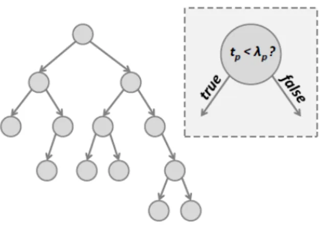
A decision tree is a classifier based on the idea of asking different questions about the data features (predictors) until reaching a decision. A tree consists of a set of nodes and a set of edges. A node of a decision tree symbolizes a question and an edge of a decision tree symbolizes an answer indicating the path to follow. The feature (predictor) that best divides the data would be represented by the root node. The classification of a new examplexstarts at the root and follows the path until reaching a terminal node (leaf node) which determines the predicted label y.
There are a lot of algorithms that defines how to construct the node function to build a decision tree. One of them is called CART [2]. It creates a binary decision tree that is constructed by splitting a node into two child nodes repeatedly, beginning with the root node that contains the whole training data S. The tree growing algorithm seeks the best split (node function) for each node. It consists in following this steps for each node n, starting from the root node (considering the case that the predictors of the feature vector are ordinal):
1. For each predictor tm of the feature vector xi = (t1,..., tM), {tm}m∈M , sort
the J different values {vj}j∈J that the predictor can take from the smallest to the
largest. Go through each value vj except the first one. Split the node according to
it using the following rule:
if tm < vj, xi goes to the left child node, otherwise, goes to the right.
The best split point λm of the predictor tm among allvj is the one that maximizes
a splitting criterion. This step finds the best split for each predictor: tm < λm, m∈M. If t is an ordinal predictor with J different values, there are J - 1 different splits on t.
2. Among all the best splits found in step 1, choose the one that maximizes the splitting criterion to find the best split of the node n: tn < λn.
3. Split the node using the split found in step 2.
not be split (there are more stopping rules that can be applied). See Figure 9 for an example.
There are several splitting criterion. The most used ones are based on the purity of the nodes such as the Gini splitting criterion or based on the entropy of the nodes.
CART algorithm uses the Gini splitting criterion: given a node n, the Gini splitting criterion is the decrease of impurity defined as
G(n) = I(n)−pL·I(nL)−pR·I(nR)
where pL and pR are the probabilities of sending a case to the left child node nL
and to the right child node nR respectively, and I(n) is the Gini impurity measure
at a node n defined as
I(n) = 1−X i∈I
p(yi|n)2 ∈[0,1[
wherep(yi|n) denotes the fraction of examples belonging to labelyi at a given node
n. Gini impurity reaches its minimum, I(n)=0, when all examples in the node have the same label.
Figure 9: Binary decision tree with its node functions tp < λp defined by CART algorithm. Image obtained from [14].
4.3
Stacked sequential learning
In many classification problems, contextual information is useful to solve ambiguous cases in classification. Stacked sequential learning algorithm takes advantage of this fact. An example of contextual information would be neighbors’ labels information or neighbors’ probabilities of belonging to one of the classes information.
[4]. A meta-learning technique uses a combination of different classifiers in order to predict a test example.
Stacked sequential learning [4] is simple to implement and can be applied to almost any base learner. It has the drawback of having a high training time.
It has been demonstrated [4] that stacked sequential learning improves the formance of non-sequential base learners and, sometimes, it also improves the per-formance of learners that are designed for sequential tasks.
Stacked sequential learning scheme is based on a two layers classifier. First of all, a classifier A is trained and tested performing a K-fold cross-validation on the original data set S. Then, an extended data set S’ is created using the original data S and the predicted labels ˆyi from the previous classification. Finally, the classifier
A is trained with this extended data S’ obtaining the model f’. The first training stage is called first step and the second training stage is called second step.
In order to test a new examplex, it must be previously extended (x’) by adding the prediction features. This procedure is done by training the base classifier A with all the data set S, testing the new example with the trained classifier f and then constructing the extended example following the same procedure as before. Once the new example is extended, it is tested using the classifier trained with S’ in the second step, which gives the final predicted labels y (y=f’(x’)).
Algorithm 1 shows the stacked sequential learning algorithm [4]. It is divided into learning algorithm, which corresponds to the training stage, and inference algorithm, which corresponds to the test stage. The first instruction of the training stage performs the K-fold cross-validation and stores each xi ∈ S joined with its
predicted label ˆyt in a set called ˆS. These predictions are then used in 2. to create
the data set S’ of extended instances x0i. Each extended example x0i is a vector containing the examplexi and the predicted labels ˆyi of the Wh previous examples
and the Wf following ones, including the predicted label yi of xi. The third step
returns the trained models f=A(S) and f’=A(S’) used in the test stage. Test stage computes in the second instruction the extended example x’ using the predictions ˆ
y=f(x) obtained in instruction number 1. Step number 3 returns the final prediction y of x.
Figure 10 shows the idea of stacked sequential learning using a graphical scheme. The procedure for extending the data in this example uses a window W of size W=Wh=Wf=2, meaning that the predicted labels from the W previous ones to the
W following ones are added to the extended data. So, this scheme shows that in the first stage, the predicted labels ˆyi are generated using the corresponding
obser-vation xi. In the second stage, the final label yi is generated by a classifier using
the observation xi and the predicted labels ˆyi−2, ˆyi−1, ˆyi, ˆyi+1 and ˆyi+2 as inputs.
Color gray in the nodes means that the node is an input for a classifier, color white means that the node is an output of a classifier, and the mix of these two colors means that the node works as an input and as an output.
Algorithm 1: Stacked Sequential Learning
P arameters: a history size Wh, a future size Wf, and a cross-validation
para-meterK.
Learning algorithm: Given a sample S = {(xi, yi)}, and a learning algorithm A:
1. Construct a sample of predictions ˆyi for each xi ∈S as follows:
(a) Split S intoK equal-sized disjoint subsetsS1,..., SK
(b) For j = 1, ..., K, let fj =A(S−Sj)
(c) Let ˆS={(xi,yˆi) : ˆyi =fj(xi) and xi ∈Sj}
2. Construct and extended data setS0 of instances (x0i, yi) by converting each
xi to x0i as follows: x
0
i = (xi,yˆi−Wh,...,yˆi+Wf)
3. Return two functions: f =A(S) and f0 =A(S0).
Inf erence algorithm: given an instance vector x: 1. Let ˆy=f(x)
2. Carry out Step 2 above to produce an extended instance x0 (using ˆy in place of ˆyi)
3. Return f0(x0)
Another version of stacked sequential learning is called multi-scale stacked se-quential learning [12]. The scheme of multi-scale stacked sese-quential learning in-cludes a new block in the scheme of stacked sequential learning. This new block defines the policy for creating the neighborhood model of the predicted labels. As before, in the multi-scale stacked sequential learning scheme a classifier is trained with the input data set S and the predicted labels ˆyi are obtained. Then, instead
of using these predicted labels to construct the extended data set S’, the new block represents the output of the classifier according to a multi-scale decomposition. Fi-nally, a grid sampling of the resulting decomposition is done to create the extended data S’. This new data set S’ is used, as before, to train a second classifier which produces the final predictions y. So the difference between stacked sequential learn-ing and multi-scale stacked sequential learnlearn-ing is the way of definlearn-ing the extended data set S’.
5
Development
In order to achieve the objectives of the work, we have developed three different methods. One is based on lumen extraction and the others two are based on a classification system.
This section explains the implementation details of each method and reports the programming language used to perform the algorithms.
5.1
LI-MA segmentation based on lumen extraction
The aim of this method is to automatically detect the LI and the MA layers of the carotid artery in the far wall using a previous lumen extraction. The method is implemented following the ideas proposed in the papers [7, 8].
The method can be divided into two parts: an approximate detection of the artery lumen and the segmentation of the LI and MA boundaries.
The lumen detection is based on the fact that the pixels belonging to the lumen have a neighborhood with specific properties. These properties are a low mean intensity and a low standard deviation. So in this part we compute, for each pixel, the mean and the standard deviation of the intensity values corresponding to its (11x11) neighborhood. Before doing that computation, we apply to the image a Gaussian filter in order to smooth it. See Figure 11 for an example. Then, we consider lumen pixels as those with a neighborhood mean intensity lower than a threshold th1=0.12 and a neighborhood standard deviation lower than a threshold th2=0.14. These parameters have been manually set using the whole training set. Once we have the image pixels classified into lumen pixel and non-lumen pixel, we need to remove as much false positives (FP) as we can. The result of the classification is represented in a binary image where 1 means lumen pixel and 0 means non-lumen pixel. To remove the FP, we perform a morphological closing on the binary image and we search for the biggest connected component, which is considered the lumen region. See Figure 12a and 12b for an example. However, it may happen that the biggest connected component is not the lumen. We correct that imposing that the lumen is the biggest connected component not being too close to the top/bottom boundaries of the image. Even doing this, still there are cases that the lumen is not detected correctly and we need to discard these cases. To achieve that, we assume that all the lumens have a similar size (area). Therefore, we compute the median of all the areas, excluding the one we are testing, and reject the lumens whose area is not close enough to the median value.
The segmentation of the LI and MA boundaries of the carotid far wall uses the result given by the lumen detection, specifically the lumen boundary which separ-ates the lumen from the far wall. This boundary is moved 0.4 mm upwards from its position in order to avoid, in some cases, that the lumen boundary includes part of
obtaining values close to zero in a region without intensity changes and obtaining high values otherwise. Afterwards, for each column of the image, we search for the point which is marked as LI. This point is the maximum of the intensity profile be-longing to the 75-th percentile and it is exactly the first maximum placed after the lumen far boundary. Then, for each column of the image, we search for the point which is marked as MA. This point is a maximum of the intensity profile belonging to the 90-th percentile and it is exactly the first maximum placed after LI point founded before. If there is not a point with these conditions, we skip the column and continue with the next one. Finally, we have for each column the LI and MA set of points and we compute the curve that best fits to each set of points so as to obtain two curves which are the estimated LI and MA boundaries respectively. We use a cubic spline for that fitting.
(a) (b)
Figure 11: Example of an image after applying the Gaussian smoothing filter. (a) Original image. (b) Smoothed image.
(a) (b) (c)
Figure 12: Example of the output of the lumen detection. (a) Original image. (b) The red region indicates the detected lumen region by the method. (c) The yellow line indicates the bottom boundary of the detected lumen and the blue line indicates the considered bottom lumen boundary after moving it upwards.
5.2
LI-MA segmentation based on a classification system
As we said at the beginning of section 5, we have performed two methods based on a classification system. The aim of these methods is to automatically detect the LI and the MA layers of the carotid artery in the far wall using a classification system, more exactly, a supervised classification system. Said in other words, these methods deals with the image segmentation problem as a classification problem. In order to work with a classification system, each pixel of the images is considered as an example of the data set. As the purpose is to segment the region inside two boundaries, the LI and the MA, there are two obvious classes/labels: inside the region formed by the LI and MA layers and outside this region. We have assigned label 1 to the pixels inside the region and label 0 to the pixels outside the region. See Figure 13a for an example. As it can be seen in Figure 13a, the pixels belonging outside the region has quite different features whether they are above the region or below the region. Therefore, another way to label the pixels is considering three classes: inside the region, above the region and below the region. We have assigned label 1 to the pixels inside the region, label 2 to the pixels above the region and label 3 to the pixels below the region. See Figure 13b for an example. Even these classifications of the pixels seem evident, we can try to verify that the pixels belonging to each label are really separable by doing a study of the features (section 5.2.1). After doing this study and choosing which labels can be used, we can proceed to implement the methods.
Both proposed methods follow the flowchart represented in Figure 14. Given the input images, first they are modified in the pre-processing step. Then, the classification step is applied to the image pixels, which is divided into two stages: the training stage and the test stage. Finally, the classification obtained goes through the post-processing step, which outputs the final segmentation.
One of the methods is the implementation of a classification system using random forest as a classifier. The other method is the implementation of a classification system using stacked sequential learning with random forest as a base learner. The second method also includes the implementation of the stacked sequential learning scheme (explained in section 4.3).
The following subsections present the feature extraction including the feature study done and explain the pre-processing step, the development of both training and test stages, and the post-processing step.
(a) (b)
Figure 13: Labels assignment. Green lines indicate the LI-MA region. (a) Case of two labels. (b) Case of three labels.
Figure 14: General flowchart of the methods based on a classification system.
5.2.1 Feature extraction
As we explained in section 4.1, before the training and test stages, there is a step we need to do: feature extraction.
The feature vectorxi of an example (pixel) is defined as a 5x5 patch of intensity
values which corresponds to the 5x5 neighborhood ofxi and itself. Therefore, given
a pixel p{i,j}, its corresponding feature vector is:
xp{i,j} = (p{i−2,j−2}, p{i−1,j−2}, ..., p{i,j}, ..., p{i+1,j+2}, p{i+2,j+2})
See Figure 15 for an example. This patch of 5x5 pixels corresponds to a patch of 0.2mm x 0.2mm.
Now that we have defined the feature vector, we can proceed to develop the study of the features. The goal of this study is to figure out if the features of the pixels from different labels are distinct enough from each other. If so, it means that the labels are separable enough so that the classifier can distinguish them properly. In order to prove that, we have done different tests with the training data S. The construction of the training data is explained in the next subsection. Each feature vector xi of the examples has 25 different features (predictors), whose values are
intensity values of the image (pixel values). We have done the tests listed below for the case of two labels and for the case of three labels:
- Plot the values of the features
In this test we have separated the training data S by labels yi. Then, for each
label, we have plotted the mean of the data values of each feature. Finally, we have put together the different graphics obtained for each label in one graphic to see the differences between the labels better. We have also included, for each label, a plot of the standard deviation of the data values of each feature in order to visualize the variability of the values. Figure 16 shows the graphic in the case of two labels and Figure 17 shows the graphic in the case of three labels.
As it can be seen in Figure 16, the both lines of the means graphics are different to each other; however, the mean data values of the label 0 are mixed with some of the mean data values of the label 1. Concretely, the variability of the label 0 is approximately from 0 to 0.55 and the variability of the label 1 is approximately from 0.15 to 0.45 (standard deviations). This is because of the high range of intensity values of the pixels belonging to label 0. If we look at Figure 13a, we can see that label 0 contains pixels very dark (the ones belonging to the lumen, above the LI-MA region) and it also includes bright pixels (the ones belonging to the far wall, below the LI-MA region). On the other hand, we can see that the pixels of the label 1 are bright but not as much as the bright ones of the label 0. Then, even though the range of each label are different, the range of the label 0 includes the range of the label 1. Therefore, the classifier could learn the features of the label 1 and distinguish them between the pixels of the label 0 that have low intensity or high intensity, but it would be hard for the classifier to differentiate the pixels of the label 0 that have intensity values similar from the intensity values of the label 1 and vice versa.
As it can be seen in Figure 17, the mean values of each label of the different means graphics are not mixed. This is due to the fact that we are considering three labels instead of two. Consequently, we are separating the bright pixels to the dark ones of the label 0. So, the labels are quite separable. However, we can see that the variability of the label 3 overlaps with the variability of the label 1, and the variability of the labels 1 and 2 are close (standard deviations). This means that the classifier could differentiate pretty good the label 1 from the label 2, but there would be some pixels of the label 3 and some pixels of the label 1 hard to classify correctly. It is harder to separate the label 1 from label 3 than from label 2 because
ude of the intensity values of the label 1 and 2.
Figure 16: Plot of the mean and the standard deviation of the data values for each feature separated by labels. The means correspond to the graphics drawn and the standard deviations are the horizontal lines. The x axis is the features (predictors) and the y axis is the intensity values. Graphic in the case of two labels. Blue corresponds to label 1 and pink corresponds to label 0. The blue lines overlap part of the pink lines because they are drawn above them.
Figure 17: Plot of the mean and the standard deviation of the data values for each feature separated by labels. The means correspond to the graphics drawn and the standard deviations are the horizontal lines. The x axis is the features (predictors) and the y axis is the intensity values. Graphic in the case of three labels. Blue corresponds to label 1, red corresponds to label 2 and green corresponds to label 3. The green lines overlap part of the blue lines because they are drawn above them.
- Histograms of the values
In this test we have separated the training data S by labels yi. Then, for each
label, we have averaged the feature vectorxi for each example of the training data.
Finally, we have computed the histogram of the examples for each label. Figure 18 shows the histograms in the case of two labels and Figure 19 shows the histograms in the case of three labels.
The histograms show us the same facts we have seen in the previous test. In the case of two labels (see Figure 18), label 0 covers almost the whole range of intensity values and, for that reason, it overlaps label 1, that has a smaller particular range of intensity values. Then, the pixels belonging to this range of values would be difficult to predict its class and this would generate errors. The same happens in the case of three labels (see Figure 19). Some of the examples of label 2 and some of the examples of label 3 overlap the region of label 1. However, as there are more examples of label 3 than label 2 that overlap label 1, there would be more errors between label 1 and 3 than between label 1 and 2. So, with this test we draw the same conclusions as before.
(a) (b)
Figure 18: Histograms in the case of two labels. Blue corresponds to label 1 and pink corresponds to label 0. The x axis is the intensity values and the y axis is the number of cases belonging to the bins. (a) Histogram of the intensity values of each example that belongs to label 1. (b) Histogram of the intensity values of each example that belongs to label 0.
(a) (b)
(c)
Figure 19: Histograms in the case of three labels. Blue corresponds to label 1, red corresponds to label 2 and green corresponds to label 3. The x axis is the intensity values and the y axis is the number of cases belonging to the bins. (a) Histogram of the intensity values of each example that belongs to label 1. (b) Histogram of the intensity values of each example that belongs to label 2. (c) Histogram of the intensity values of each example that belongs to label 3.
To sum up, we have seen that the different labels are quite separable in both options (using two labels and using three labels). For that reason, we have chosen both options to work with and all the tests have been performed for both cases. However, we have also seen that there are overlaps between the data of the differ-ent labels. This will difficult the classification of some examples and will make the segmentation a challenging task.
5.2.2 Pre-processing step
This step modifies the input images in order to ease the classification. They are converted to gray scale. They are also equalized, which means that their intensity values are mapped in order to cover the entire possible range of values. This en-hances their contrast. In addition, the images are normalized to the range [0 1]. Finally, the images are smoothed using a Gaussian smoothing filter (see Figure 11) to reduce the pronounced differences between the intensity values.
5.2.3 Classification system: training stage
After defining the feature vector (section 5.2.1), we need to know which pixels of the image are going to be part of the training data. Said in other words, we have to choose the examples for the training data S. In order to do this, we have to define a region of the image that comprises a balanced percentage of examples for each label
yi. Then, the pixels inside this region are the examples that compose the training
data. This region is called region of interest (ROI).
We have defined two different ways of choosing the training ROI for the training data based on the ground truth (GT) of the images (section 6.1). The first one consists in building a rectangle that comprises the pixels inside the GT and some more pixels above and below it. The right and left boundaries of the rectangle are defined by the right and left limits of the GT respectively. The top and bottom boundaries of the rectangle are defined by finding the lower row of the image and the higher row of the image that covers the GT and then decreasingθ1 mm the lower
row and increasingθ1mm the higher row to include more pixels of the outside of the
GT. See Figure 20a for an example. The second ROI also consists in constructing a region that comprises the pixels inside the GT and some more pixels above and below it. But in this case the ROI is not a rectangle. The ROI definition consists in dilating θ2 mm the top and bottom boundaries of the GT in order to keep its
form for the ROI. The right and left boundaries of the ROI are the right and left limits of the GT respectively, as in the first ROI. See Figure 20b for an example.
If we consider all the pixels of the ROI as belonging to the training data, there would be too much examples to compute. Thus, we define a sub-sampling by choosing 1 of every 10 pixels of the ROI.
To decide how many millimeters (mm) we need to dilate the rectangle that comprises the GT in the first ROI (θ1), and how many mm we need to increase the
boundaries of the second ROI (θ2), we have to choose those mm values that generate
a balanced training data. In order to verify that, we have computed the percentage of each label yi in the training data S defined by the ROI and the sub-sampling.
Table 4 shows the percentages obtained for the definitive ROIs (θ1 = 0.4mm and
θ2 = 0.8mm) in the case of two labels and Table 5 in the case of three labels.
train-(a) (b)
Figure 20: Example of the definition of the ROIs in the training stage. (a) Image of the first training ROI explained in the text. Green corresponds to GT, blue corresponds to the ROI obtained and the red points represent the lower and the higher rows of the GT, which are used as a reference to build the rectangle. The vertical distance between the red point and the rectangle is θ1. (b) Image of the
the second training ROI explained in the text. Green corresponds to GT, blue corresponds to the ROI obtained. The vertical distance between blue and green lines (top and bottom) for each column of the image isθ2.
ROI 1 ROI 2
Percentage of labels 1 43% 43.2% Percentage of labels 0 57% 56.8%
Table 4: Percentage of each label in the training data S depending on the ROI used.
Case of two labels. ROI 1 refers to the first ROI explained in section 5.2.3 and ROI 2 refers to the second one.
ROI 1 ROI 2
Percentage of labels 1 43% 43.2% Percentage of labels 2 33% 28.6% Percentage of labels 3 24% 28.2%
Table 5: Percentage of each label in the training data S depending on the ROI used.
Case of three labels. ROI 1 refers to the first ROI explained in section 5.2.3 and ROI 2 refers to the second one.
5.2.4 Classification system: test stage
As in the previous subsection, once we have defined the feature vector of the test examples (section 5.2.1), we need to define which pixels of the image are going to form the test data. So, we have to choose a ROI for the test data.
We have defined three different test ROIs. As we are in the test stage, we cannot use the GT of the image that is being tested, but we can use the GT of the other images. So, these three ROIs are based on the GT of the training images. The first ROI follows the idea of the first ROI explained for the training data. The test ROI is a rectangle built using the information of the lumen extraction (explained in section 5.1) and the information of the ROIs of the training images (the first training ROI explained). First, for each training image, given the bottom boundary of the lumen detected of an image, we select a point of this lumen boundary and we compute how many pixels separate this point from the bottom of the image ROI vertically (differences down) and how many pixels separate the lumen boundary from the top of the image ROI vertically (differences up). See Figure 21a for an example. Then, we compute the maximum of both differences up and differences down computed for the training ROIs. Given the bottom boundary of the lumen of the test image, we define the top and the bottom boundaries of the ROI adding the maximum of differences up above the lumen boundary and adding the maximum of differences down below the lumen boundary. Finally, we define the left and right boundaries of the ROI as the ones of the left and right boundaries of the training ROIs respectively that construct the widest rectangle. The second ROI is defined as the first one but using the second type of training ROI explained instead of the first type. As before, we compute the differences up and the differences down. See Figure 21b for an example. Then, rather than create a rectangle, we dilate the bottom lumen boundary the maximum of differences up above and the maximum of differences down below to keep its form. The right and left boundaries of the ROI are defined in the same way as before. The last ROI we create uses the method developed for the segmentation based on lumen extraction (section 5.1). The top boundary of the ROI is the LI layer found by the method moved some mm above and the bottom boundary of the ROI is the MA layer found by the method moved some mm below. The right and left boundaries are defined as the other two ROIs. Once the feature vector and the test ROI are defined, we can construct the test data and predict the labels y of the test examples x using the model f learned in the previous stage: y=f(x).
(a) (b)
Figure 21: Example of the definition of the ROIs in the test stage. (a) Training image used to construct the first test ROI explained in the text. (b) Training image used to construct the second test ROI explained in the text. In both cases, blue corresponds to a ROI obtained in the training stage, red corresponds to the lumen detection output, the yellow point R represent the point selected of the bottom lumen boundary used as a reference to compute the differences up and differences down, differences up = R-A and differences down = B-R.
5.2.5 Post-processing step
This step refines the result obtained with the classification system. Given a mask with the classification result for the label 1, we first fill the holes. See Figure 22a and Figure 22b for an example. Then, we use morphological opening and closing operations to create connected components. See Figure 22c and Figure 22d. The structuring element for these operations is an horizontal rectangle. The dimensions of each rectangle have been manually set testing different values and choosing the best for the whole training set. In further experiments, new values should be es-timated by cross validation. Finally, we choose the connected component that has points belonging to the middle row of the ROI. See Figure 22e and Figure 23. We can make this assumption because the ROI is defined so that the pixels belonging to the label 1 are placed in the middle rows of the ROI. Therefore, there will be pixels labeled as 1 in the middle row of the ROI in the majority of cases.
(a) (b)
(c) (d) (e)
Figure 22: Post-processing example. (a) Mask with the classification result for the label 1 (without post-processing). (b) Fill holes step output. (c) Opening operation output. (d) Closing operation output. (e) Final output of the post-processing step.
Figure 23: Example of a mask with the classification result with its ROI painted in blue. The red line corresponds to the middle row of the ROI.
5.3
Programming language
MATLAB (abbreviation of MATrix LABoratory) is a high-level technical comput-ing language and interactive environment for algorithm development, data visual-ization, data analysis, and numerical computation. As the name suggest, its basic element of data is a matrix that does not require dimensioning. This allows solv-ing many technical computsolv-ing problems in much less time than it would take to run a program written in another language. So MATLAB is oriented to matrix manipulations, besides plotting functions and data, implementation of algorithms and many other interesting features. MATLAB is equipped with multiple toolboxes that increase its functionality and enhance its power.
As we work with images and MATLAB represents images using matrices, we have chosen this programming language because of its flexibility when working with matrices and vectors, its image processing toolbox and its statistics toolbox that can be used to solve supervised machine learning problems. We have worked with MATLAB R2014a release.
6
Experimental results
In this section, we introduce the considered data set, we define the validation meas-ures used to evaluate each of the methods implemented, we present the results obtained and we discuss them. The execution time for each of the methods is also shown.
6.1
Data set
We consider a data set from REGICOR, Girona’s Heart Registry, created with 30 subjects.
As explained in paper [21], the 30 subjects from REGICOR data set were part of the cohort of a longitudinal study conducted at the project Girona Heart Registry. The images were collected from 2007 to 2010. The subjects were aged between 35 and 84, and those with a history of previous cardiovascular disease were excluded. Two trained sonographers performed the carotid artery ultrasound scans with an Acuson XP128 ultrasound system equipped with L75-10 MHz transducer and a computer program extended frequency (Siemens-Acuson, Mountainview, Califor-nia, United States). Ultrasound longitudinal images were obtained in B-mode from CCA with resol


![Figure 10: Stacked sequential learning scheme, W=2. Image obtained from [4].](https://thumb-us.123doks.com/thumbv2/123dok_us/779105.2598529/27.892.257.634.815.1028/figure-stacked-sequential-learning-scheme-w-image-obtained.webp)