Mining Association Rules for Label Ranking
Cl´audio S´a1, Carlos Soares1,2, Al´ıpio M´ario Jorge1,3, Paulo Azevedo5, and Joaquim Costa4
1
LIAAD-INESC Porto L.A., Rua de Ceuta 118-6, 4050-190, Porto, Portugal 2
Faculdade de Economia, Universidade do Porto 3 DCC - Faculdade de Ciˆencias, Universidade do Porto
4
DM - Faculdade de Ciˆencias, Universidade do Porto 5 CCTC, Departamento de Inform´atica, Universidade do Minho
claudio@liaad,up.pt, [email protected], [email protected], [email protected], [email protected]
Abstract. Recently, a number of learning algorithms have been adapted for label ranking, including instance-based and tree-based methods. In this paper, we continue this line of work by proposing an adaptation of as-sociation rules for label ranking based on the APRIORI algorithm. Given that the original APRIORI algorithm does not aim to obtain predictive models, two changes were needed for this achievement. The adaptation essentially consists of using variations of the support and confidence mea-sures based on ranking similarity functions that are suitable for label ranking. Additionally we propose a simple greedy method to select the parameters of the algorithm. We also adapt the method to make a pre-diction from the possibly conflicting consequents of the rules that apply to an example. Despite having made our adaptation from a very simple variant of association rules for classification, partial results clearly show that the method is making valid predictions. Additionally, they show that it competes well with state-of-the-art label ranking algorithms.
1
Introduction
Label ranking is an increasingly popular topic in the machine learning litera-ture [10, 6, 22]. Label ranking studies the problem of learning a mapping from instances to rankings over a finite number of predefined labels. It can be consid-ered as a variant of the conventional classification problem, where only a single label is requested instead of a ranking of all labels [6]. In contrast to a classifi-cation setting, where the objective is to assign examples to a specific class, in label ranking we are interested in assigning a complete preference order of the labels to every example.
There are two main approaches to the problem of label ranking that we may refer to as decomposition and direct methods. Decomposition methods decom-pose the problem into several simpler problems (e.g., multiple binary problems).
Direct methods adapt existing algorithms or develop new ones to treat the rank-ings as target objects without any transformation. An example of the former is the ranking by pairwise comparisons of [10]. Examples of algorithms that were
adapted to deal with rankings as the target objects include decision trees [20, 6], k-Nearest Neighbor [4, 6] and the linear utility transformation [11, 7]. This second group of algorithms can be divided into two approaches. The first one contains methods (e.g., [6]) that are based on statistical distributions of rank-ings, such as Mallows [14]. The other group of methods are based on measures of similarity or correlation between rankings (e.g., [20, 2]).
In this paper, we propose an adaptation of the association rule mining al-gorithm APRIORI for label ranking based on similarity measures. Association rules mining is a very important and successful task in data mining. Although the original algorithm was developed for descriptive tasks, several adaptations have been proposed for predictive problems.
The paper is organized as follows: sections 2 and 3 introduce the label ranking problem and the task of association rule mining, respectively; section 4 describes the algorithm proposed here; section 5 presents the experimental setup and dis-cusses the results; finally, section 6 concludes this paper.
2
Label Ranking
The formalization of the label ranking problem given here follows the one pro-vided in [6].6 Label ranking can be considered as a variant of the conven-tional classification task. In classification, given an instancexfrom the instance space X, the goal is to predict the label (or class) λ from a pre-defined set
L = {λ1, . . . , λk} to which x belongs. In label ranking the goal is to predict the ranking of the labels in L that are associated withx. We assume that the ranking is a total order over L defined on the permutation space Ω. Alterna-tively, we may say that λa x λb indicates that λa is preferred to λb given the instance x. A total order x can be seen as a permutation π of the set {1, . . . , k}, such that π(a) is the position of λa in π.7 Let us also denote π as the result of inverting the order inπ. As in classification, we do not assume the existence of a deterministic X→Ωmapping. Instead, every instance is
associ-ated with a probability distribution over Ω. This means that, for each x ∈ X,
there exists a probability distributionP(·|x) such that, for everyπ∈Ω,P(π|x) is the probability that π is the ranking associated with x. The goal in label ranking is to learn the mappingX→Ω. The training data is a set of instances T = (Tx, Tπ) = {xi, πi}, i = 1, . . . , n, where xi are the independent variables describing instanceiandπi is the corresponding target ranking.
Given the ranking ˆπ predicted by a label ranking model for an instance x, which is, in fact, associated with the true label rankingπ, we need to evaluate the accuracy of the prediction. For that, we need a loss function onΩ. One such function is the number of discordant label pairs,
D(π,ˆπ) = #{(i, j)|π(i)> π(j)∧π(i)ˆ <ˆπ(j)} (1) 6
An alternative formalization can be found in [21]. 7
which, if normalized into the interval [−1,1], will give the Kendall’sτcoefficient. The latter is as a correlation measure whereD(π, π) = 1 andD(π, π) =−1. We obtain a loss function by averaging this function over a set of examples. We will use it as evaluation measure in this paper, as it has been used in recent studies [6]. However other distance measures could have been used, like Spearman’s rank [18] correlation.
3
Association Rules Mining
An association rule (AR) is an implication of the form: A→C
where A, C⊆Xand ATC =∅.8 Association rules are typically chacterized by
two measures, support and confidence. The support of ruleA→CinT issupif sup% of the cases in it containAandC. Additionally, it has a confidenceconf in T ifconf% of cases inT that containAalso containC.
The original method for induction of AR is the APRIORI algorithm that was proposed in 1994 [1]. We describe this algorithm in the following section. Association rules were originally proposed for descriptive purposes. However, they have been adapted for predictive tasks such as classification (e.g., [15]). Given that label ranking is a predictive task, we describe some useful notation from an adaptation of AR for classification in Section 3.2.
3.1 APRIORI Algorithm
APRIORI identifies all AR that have a support and confidence higher than a given minimal support threshold (minsup) and a minimal confidence threshold (minconf), respectively. Thus, the model generated by APRIORI is a set of AR of the form A → C, where A, C ⊆ X, and sup(A∪C) ≥ minsup and
sup(A∪C)/sup(A)≥minconf.
APRIORI mining process can be divided into three steps: Candidate gen-eration, Candidate support count and Rule Generation. The first, Candidate generation, takes advantage of a simple restriction called thedownward closure property which states that anitemsetis considered frequent if, and only if, all of itssub-itemsets are frequent. Hence, it uses one generation of frequentitemsets (of length k) to build the next generation (of length k+1). This is why the algorithm was named APRIORI: at each step, it works with from candidates obtained a priori. The pseudo-code is given in Algorithm 1.
The second,Candidate support countscans the data to determine the support of the generated itemsets. For simplicity reasons, support is here expressed as
8
To simplify notation, we assume that an itemset, usually referred to in the AR literature asI, is equivalent to an instance space Xin label ranking. Although this
is not exactly true, a simple parallel can be established between the two concepts, and thus, this does not affect the correctness of the paper.
Algorithm 1APRIORI Candidate generator - APRIORIGen
Require: Fk Ck+1=∅
for allf1, f2∈Fkdo
if f1= (i1, . . . , ik−1, ik) andf2= (i1, . . . , ik−1, i∗) :∀ik< i∗then c=f1∪f2= (i1, . . . , ik−1, ik, i∗) if c− {i} ∈Fk,∀i∈cthen Ck+1=Ck+1∪c end if end if end for return Ck+1
support count, which is simply the number of times anitemsetcan be found in the dataset. First, it scans the data to count the1-itemsets, i∈Tx. If one ore more exceedsminsupthen the item becomes a frequent 1-itemset.
In summary, the APRIORI algorithm consists of, at each stepk, using the
APRIORIGen step to generatek−candidates, and the support count setp to prune the set of itemsets with respect to the user definedminsup. The algorithm is summarized in Algorithm 2.
Algorithm 2APRIORI
Require: minsup
Ck: Candidate itemset of sizek Fk: Frequent itemset of sizek Tx: Transactions in the database
F1={frequent itemsets of lenght 1 inTx}
fork= 1;Fk6=∅;k+ +do Fk+1=∅ Ck+1= APRIORIGen(Fk) for allt∈T do for allc∈Ck+1do if c⊆tthen sup(c) =sup(c) + 1 end if end for end for Fk+1={c:c∈Ck+1∧sup(c)≥minsup} end for return ∪kFk,∀k
The final partRule Generation (Algorithm 3), splits every frequentitemset into all possible combinations of two non-emptysub-itemsets in order to obtain rules from it. This will result in anantecedent and aconsequent of a rule, which
will have its confidence value (conf) compared to the user specified threshold minconf.
Algorithm 3Rule generation
Require: minconf andFk
for allf∈Fk;k≥2do
for alla⊆f;length(a)≤k−1do
c=f\ {a}
conf(a→c) = supsup((fa))
if conf(a→c)≥minconf then return a→c
end if end for end for
Despite the usefulness and simplicity of APRIORI, it runs a time consuming candidate generation process and needs space and memory proportional to the number of possible combinations in the database. Additionally it needs multiple scans of the database and typically generates a very large number of rules. Be-cause of this, many new pruning methods were proposed in order to avoid that. Such as the hashing technique [16], dynamic itemset counting [5], parallel and distributed mining [17], relational database systems integrated with mining [19] which reduces the number of database scans.
3.2 Class Association Rules
As stated earlier, AR were originally proposed for descriptive purposes. However, given that label ranking is a prediction task, we need to adapt their definition for that purpose. Our adaptation is based on Classification Association Rules (CAR), proposed as part of the Classification Based on AR (CBA) algorithm [15].
A class association rule (CAR) is an implication of the form: A→λ
where A ⊆ X, and λ∈ L, which is the class label. The rules can also be
rep-resented as hcondset, λi, where condset =A.9 A rule A → λ holds in T with confidenceconf ifconf% of cases inT that containAare labelled with classλ. And with supportsupinT ifsup% of the cases in it containAand are labelled with classλ.
CBA takes a tabular data setT = (Tx, Tλ) ={xi, λi}, where xi is a set of items and λi the corresponding class, and look for all ruleitems of the form hcondset, λi. The algorithm aims to choose a set of high accuracy rules R to
9
match Tx. An instancexi ∈Tx is considered matched by R if at least one rule (A→λ)∈R, withA⊆xi, and λ∈ L. If the rules can’t classify all examples, a default class is given to them (e.g., the majority class in the training data).
4
Association Rules for Label Ranking
We define aLabel Ranking Association Rule (LRAR) as a straightforward adap-tation of class association rules (CAR):
A→π
whereA⊆X, andπ∈Ω. The only difference is that the labelλ∈ Lis replaced
by the ranking of the labels,π∈Ω. Similar to what the predicton made in CBA, when an exemple matches the ruleA→π, the predicted ranking isπ.
4.1 Direct Implementation
A straightforward application of the CBA algorithm to the label ranking method can be made by considering each unique permutation π ∈ Ω as a class. More generally, the number of classes will be the number of distinct π ∈ Ω. Under this assumption we are able to directly use the CBA, or, in fact, any other classification algorithm, on label ranking data sets.
An example of how the data can be displayed for this problem is given in Table 1.
Table 1.An example of a label ranking dataset to be processed by a AR-based classi-fication algorithm. TID represents the identifier of the example (the transaction in AR terminology)
TID A1 A2 A3 λi
1 L XL S (2,3,1)
2 XXL XS S (2,1,3)
3 L XL XS (1,3,2)
The support count of condset (sup(condset))is the number of cases in Tx that contain the condset, and for ruleitem (sup(hcondset, π >)) is the number of cases inT that contain thecondset and have the rankingπassociated. Thus, theconfidence will be:
conf(hcondset→πi) =sup(hcondset, πi)
sup(condset) (2)
A rule A → λ holds in T with confidence conf if conf% of cases in T that containA are labelled with classλ. And with supportsupin T ifsup% of the cases in it containAand are labelled with classλ.
Drawbacks This approach has two important problems. First, the number of classes can be extremely large, up to a maximum of k!, wherek is the length of the set of labels, L. For instance, if the number of labels is 5, the number of permutations is 5! = 120. This means that the amount of data required to learn a reasonable mappingX→Ω is too big.
The second disadvantage is that this approach does not take into account the differences in nature between label rankings and classes. In classification, two examples either have the same class or not. In this regard, label ranking is more similar to regression than to classification. Given an example with a target value of 5, another example with a target value of 5.1 is more similar to it than one with a target value of 4 (at least, in terms of the target values).
This property can be used in the induction of prediction models. Again, let us consider the case of regression. A large number of observations with a given target value, say 5.3, increases the probability of observing similar values, say 5.4 or 5.2, but not so much for very different values, say -3.1 or 100.2. A similar reasoning can be made in label ranking. Let us consider the case of a data set in which ranking πa ={A, B, C, D, E} occurs in 1% of the examples. Treating rankings as classes would mean that P(πa) = 0.01. Let us further consider that the rankings πb ={A, B, C, E, D}, πc = {B, A, C, D, E} and πd ={A, C, B, D, E} occur in 50% of the examples. Taking into account the stochastic nature of these rankings [6],P(πa) = 0.01 seems to underestimate the probability of observing πa. In other words it is expected that the observation ofπb,πcandπdincreases the probability of observingπa and vice-versa, because they are similar to each other.
This affects even rankings which are not observed in the available data. For example, even though πe = {A, B, D, C, E} is not present in the data set it would not be entirely unexpected to see it in future data.
4.2 Support and Confidence for Label Ranking
To take this characteristic into account, we can argue that the support of a rank-ing πincreases with the observation of similar rankings and that the variation is proportional to the similarity. Given a measure of similarity between rankings s(πa, πb), we can adapt the concept of support of the ruleitem hcondset, πi as follows:
suplr(hcondset, πi) =
X
i:condset⊆xi
s(πi, π)
n (3)
Essentially, what we are doing is assigning a weight to each target ranking in the training,πi, data that represents its contribution to the probability that π may be observed. Someitemsets give full contribution to the support count (i.e., 1), while others give partial or even a null contribution.
Any function that measures the similarity between two rankings or permu-tations can be used, such as Kendall’sτ [13] or Spearman’sρ[18]. The function
used here is of the form:
s(πa, πb) =
s0(πa, πb) ifs0(πa, πb)≥θ
0 otherwise (4)
where s0 is a similarity function. This general form assumes that below a given threshold, θ, is not useful to discriminate between different similarity values, as they are so different from πa. This means that, the support sup of the ruleitem=hcondseta, πaiwill have contributions from all theruleitems of the form hcondseta, πbi, for allπb wheres0(πa, πb)> θ). Again, many functions can be used ass0.
The confidence of a rule condset → π is obtained simply by replacing the measure of support with the new one.
conflr(hcondset, πi) =
suplr(hcondset, πi)
sup(condset) (5)
Given that the loss function that we aim to minimize is known beforehand, it makes sense to use it to measure the similarity between rankings. Therefore, we use Kendall’sτ. In this case, we think that θ= 0 would be a reasonable value, givent that it separates the negative from the positive contributions. Table 2 shows an example of a label ranking dataset represented following this approach.
Table 2.An example of a label ranking dataset to be processed by the APRIORI-LR algorithm. π1 π2 π3 TID A1 A2 A3 (1,3,2) (2,1,3) (2,3,1) 1 L XL S 0.33 0.00 1.00 2 XXL XS S 0.00 1.00 0.00 3 L XL XS 1.00 0.00 0.33
To present a more clear interpretation, the example given in table 1, the
condset (L, XL, S) (TID=1) contributes to the the support count of the itemset (L, XL, S, π1) with 1. The same example, in the table 2 will also give a small contribution of 0.33 to the support count of the itemset (L, XL, S, π3), given their similarity. On the other hand, in both cases, no contribution is given to the count of the itemset’s (L, XL, S, π2) support, which are clearly different.
4.3 APRIORI-LR Algorithm
Using the definitions of support and confidence proposed, adaptation of APRI-ORI for label ranking is simple. Given a training setT = (Tx, Tπ) ={xi, πi}, i= 1, . . . , n, frequentitemsets are generated with Algorithm 4 onT. These consist of both regular itemsets and itemsets with one complete ranking included. Then,
the adapted version of the Rule generator, the Algorithm 5, will be used to make the rules based on this last group. The first group will be ignored.
For the generation of frequent itemsets it was used the CAREN [3] software.
Algorithm 4APRIORI-LR - APRIORI for Label Ranking pseudo-code
Require: minsup
Ck: Candidate itemset of sizek Fk: Frequent itemset of sizek
T = (Tx, πi): Transactions in the database F1={frequent itemsets of lenght 1 inTx}
fork= 1;Fk6=∅;k+ +do
Fk+1=∅
Ck+1= APRIORIGen(Fk)
for allt∈T wheret={tx, πx}do
for allc∈Ck+1do
if c⊆txthen sup(c) =sup(c) + 1
else if c⊆tthen
sup(c) =sup(c) +suplr(c)
end if end for end for Fk+1={c:c∈Ck+1∧sup(c)≥minsup} end for return ∪kFk,∀k
Algorithm 5Rule generation for APRIORI-LR
Require: minconf andFk
for allf∈Fk;k≥2do
if anyi⊆f:i∈Ωthen
fx=f\ {π}
conf(fx→π) = supsup(f(xf→π)
x)
if conf(f→π)≥minconf then return f→π
end if end if end for
LetRlr be the set of all the generated label ranking association rules. The algorithm aims to create a set of high accuracy rulesrlr∈ Rlr to coverTx. The classifier has the following format:
However, if these are insufficient to rank the given examples, adef ault ranking will be used. The default ranking can be the average ranking [4].
This approach has two problems. The first is that it can only predict rankings which were present in the training set. The second problem is that it solves conflicts between rankings without taking into account the “continuous” nature of rankings, which was illustrated earlier. The problem of generating a single permutation from a set of conflicting rankings has been studied in the context ofconsensus rankings.
It has been shown in [12] that a ranking obtained by ordering the average ranks of the labels across all rankings minimizes the euclidean distance to all those rankings. In other words, it maximizes the similarity according to Spear-man’sρ[18]. Givenmrankingsπi(i= 1, . . . , m) we aggregate them by comput-ing for each item j (j = 1, . . . , k)
rj= m P i=1 πi,j m (6)
The predicted ranking ˆπis obtained by ranking the itens according to the value ofrj.
We can take advantage of this in the ranker builder in the following way: the final predicted label ranking is the consensus of all the label rankings in the consequent of the rulesrlr triggered by the test example.
4.4 Matching Maximization
Due to the intrinsic nature of each different dataset, or even of the pre-processing methods used to prepare the data (e.g., the discretization method), the maximum
minsup/minconf needed to obtain a rule setRlrthat matches all or at least most of the examples, may vary significantly.
Before the experiment tests we use a greedy method to define the minimum confidence. As stated earlier, a rule set Rlr matches an example if at least one rule (A → λ) ∈ Rlr, with A ⊆ xi. Then, our goal is to obtain a rule set Rlr that maximizes the number of examples that are matched. Additionally, we want that Rlr contains the best rules. In other words, we want the rules with high confidence values.
The matching maximization method (Algorithm 6) will determine theminconf that obtains the rule set according to those criteria. Then the 10-fold cross val-idation will be started taking into account this value. The 5% step is somewhat arbitrary. From the efficiency point of view, a suitableminconf must be found as soon as possible. On the other hand, this very same value should be as high as possible. As a result, 5% seems a reasonable step.
The ideal value for theminsup, is the nearest to 1However, in some datasets, namely those with a great number of attributes, the frequent itemset generation can be a heavy time consuming task. In this case, the results wont have the
minsup set to 1%. In this work, one such example is theauthorship, wich has 70 attributes.
Algorithm 6Matching Maximization Algorithm M = 0 minconf= 100% minsup= 1 whileM <100%do minconf=minconf−5%
Run the algorithms 4 and 5 withminsupandminconf and determine the per-centage of examples matched,M
end while
return minsup, minconf
This procedure has the important advantage that it does not take into ac-count the accuracy of the rule sets generated.
5
Experimental Results
Here, we start by describing the datasets used, then we present the experimental setup and, finally, we present and discuss results.
5.1 Datasets
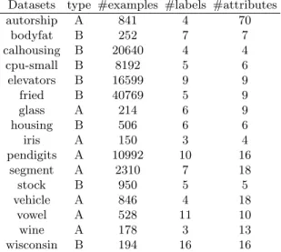
The data sets in this work were taken from KEBI Data Repository in the Philipps University of Marburg, which were also used in the experimental work presented in [6]. Some information is provided in Table 3.
Two types of methods were used to generate these label data sets: (type A) the target ranking is a permutation of the classes of the original target attribute, derived from the probabilities generated by a naive Bayes classifier; (type B) the target ranking is derived for each example from the order of the values of a set of numerical variables, which are no longer used as independent variables. Despite it may seem a little arbitrary, the original attributes are correlated so the remaining independent variables will also contain information about these artificial created rankings.
Continuous variables were discretized by two distinct methods: (1) recur-sive minimum entropy partitioning criterion ([9]) with theminimum description length (MDL) as stopping rule, motivated by [8] and (2)equal width bins.
The first method, in some cases, was not able to find a partition for some attributes. As we are dealing with AR discovery, these attributes would origin a sup= 100%. This means that they are present in all frequent item sets. Despite the fact that it does not affect the accuracy of the algorithm, it would slow down the process of finding ARs, so they were removed. For the cases were all attributes were removed due to this reason, the results are not applicable (na).
5.2 Experimental Setup
The evaluation measure is Kendall’s τ and the performance of the method was estimated using ten-fold cross-validation.
Table 3.Summary of the datasets
Datasets type #examples #labels #attributes
autorship A 841 4 70 bodyfat B 252 7 7 calhousing B 20640 4 4 cpu-small B 8192 5 6 elevators B 16599 9 9 fried B 40769 5 9 glass A 214 6 9 housing B 506 6 6 iris A 150 3 4 pendigits A 10992 10 16 segment A 2310 7 18 stock B 950 5 5 vehicle A 846 4 18 vowel A 528 11 10 wine A 178 3 13 wisconsin B 194 16 16
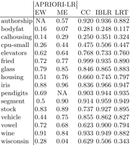
The performance of APRIORI-LR is compared with a baseline method, the default ranking explained earlier. Additionally, we compare the performance of our algorithm with the results obtained with constraint classification (CC), instance-based label ranking (IBLR) and ranking trees (LRT), that were pre-sented in [6]. However, we note that we did not run experiments with these methods and simply compared our results with the published results of the other methods. Thus, they were probably obtained with different partitions of the data and can not be compared directly. However, they provide some indication of the quality of our method, when compared to the state-of-the-art.
5.3 Results
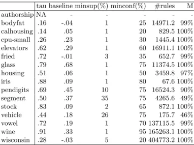
In Tables 4 and 5, the minsup and minconf presented are the values obtained when theM reached approximately 100% as shown in columnM. Some of them were stopped with a value ofM slightly less then that because of the computa-tional costs in terms of time consumption.
The tables show that the method obtains results that are clearly better than the ones obtained by the baseline method with both discretization methods. This means that the APRIORI-LR is identifying valid patterns that can predict label rankings.
As stated earlier, we compare APRIORI-LR with state-of-the-art methods, based on results published in [6], just to get a rough idea of the quality of the proposed method. These results show that APRIORI-LR is a competitive method. We note that APRIORI-LR is a simple adaptation of APRIORI for label
Table 4.Results obtained withminimum entropy discretization
tau baseline minsup(%) minconf(%) #rules M
authorship .57 .57 50 50 9.0 100% bodyfat .07 -.04 1 15 3203.3 97% calhousing .29 .05 1 35 207.9 96% cpu-small .44 .23 1 35 2643.6 100% elevators .64 .29 1 60 1779.5 97% fried .77 -.01 1 35 1910.1 97% glass .85 .67 1 85 465.1 99% housing .76 .06 1 60 2502.9 97% iris .96 .09 1 90 114.4 100% pendigits na - - - - -segment .90 .37 1 85 633123.6 100% stock .89 .09 1 80 1126.6 99% vehicle .75 .18 1 85 2535.5 100% vowel .68 .20 1 70 20642.8 99% wine .84 .33 15 95 5877.0 100% wisconsin .04 -.03 1 0 1227.0 93%
Table 5.Results obtained withequal widthdiscretization with 3 bins for each attribute
tau baseline minsup(%) minconf(%) #rules M
authorship NA - - - - -bodyfat .16 -.04 1 25 14971.2 99% calhousing .14 .05 1 20 829.5 100% cpu-small .26 .23 1 30 1445.4 100% elevators .62 .29 1 60 16911.1 100% fried .72 -.01 3 35 652.7 99% glass .79 .68 1 75 11374.5 100% housing .51 .06 1 50 3459.8 97% iris .88 .09 1 80 67.6 100% pendigits .69 .45 10 75 16524.3 90% segment .50 .37 35 75 4265.6 49% stock .83 .09 2 65 872.1 100% vehicle .44 .18 26 75 175.7 46% vowel .72 .19 1 70 137115.5 99% wine .91 .33 1 95 165263.1 100% wisconsin .28 -.03 5 20 404773.2 100%
Table 6.Comparison of APRIORI-LR with state-of-the-art methods. APRIORI-LR results obtained withequal width discretization with 3 bins for each attribute
APRIORI-LR EW ME CC IBLR LRT authorship NA 0.57 0.920 0.936 0.882 bodyfat 0.16 0.07 0.281 0.248 0.117 calhousing 0.14 0.29 0.250 0.351 0.324 cpu-small 0.26 0.44 0.475 0.506 0.447 elevators 0.62 0.64 0.768 0.733 0.760 fried 0.72 0.77 0.999 0.935 0.890 glass 0.79 0.85 0.846 0.865 0.883 housing 0.51 0.76 0.660 0.745 0.797 iris 0.88 0.96 0.836 0.966 0.947 pendigits 0.69 NA 0.903 0.944 0.935 segment 0.5 0.90 0.914 0.959 0.949 stock 0.83 0.89 0.737 0.927 0.895 vehicle 0.44 0.75 0.855 0.862 0.827 vowel 0.72 0.68 0.623 0.900 0.794 wine 0.91 0.84 0.933 0.949 0.882 wisconsin 0.28 0.04 0.629 0.506 0.343
ranking. We expect that the results can be significantly improved, for instance, by implementing more complex pruning methods.
6
Conclusions
In this paper we present a simple adaptation of the APRIORI algorithm for label ranking. This adaptation essentially consists of 1) enforcing rules to have label rankings in their consequent, 2) using variations of the support and confidence measures that are suitable for label ranking and 3) generating the model with parameters selected by a simple greedy algorithm.
These results clearly show that this is a viable label ranking method. It clearly outperforms a simple baseline, which means that, despite its simplicity, it is inducing useful patterns.
Additionally, the results obtained indicate that the choice of the discretiza-tion method and the number of bins per attribute, play an important role in the efficiency. The tests indicate that the supervised discretization method, ( min-imum entropy, gives better results than the equal width partitioning. This is, however, not the main focus of this work.
This work uncovered several possibilities that could be better studied in or-der to improve the algorithm’s performance. Some of the most important are improvements to the methods for prediction generation and matching maxi-mization. Additionally, it is essential to implement some model pruning method. Improvements can also be achieved by adapting the discretization method, the
choice of the measure of similarity sin conjunction with the parameter θ and the use of different measures for the improvement of APRIORI-LR.
In terms of real world applications, these can be adapted to rank analysts, based on their past performance and also radios, based on user’s preferences.
Acknowledgment
This work was partially supported by FCT project Rank! (PTDC/EIA/81178/2006) and Palco AdI project Palco3.0 financed by QREN and Fundo Europeu de De-senvolvimento Regional (FEDER). We thank the anonymous referees for useful comments.
References
1. Agrawal, R., Srikant, R.: Fast algorithms for mining association rules. In: Proc. 20th Int. Conf. Very Large Data Bases, VLDB. vol. 1215, p. 487499. Citeseer (1994) 2. Aiguzhinov, A., Soares, C., Serra, A.P.: A similarity-based adaptation of naive
bayes for label ranking. In: Discovery Science (2010)
3. Azevedo, P.: CAREN-A java based apriori implementation for classification pur-poses (2003)
4. Brazdil, P., Soares, C., Costa, J.: Ranking Learning Algorithms: Using IBL and Meta-Learning on Accuracy and Time Results. Machine Learning 50(3), 251–277 (2003)
5. Brin, S., Motwani, R., Ullman, J.D., Tsur, S.: Dynamic itemset counting and im-plication rules for market basket data. Proceedings of the 1997 ACM SIGMOD in-ternational conference on Management of data - SIGMOD ’97 pp. 255–264 (1997), http://portal.acm.org/citation.cfm?doid=253260.253325
6. Cheng, W., H¨uhn, J., H¨ullermeier, E.: Decision tree and instance-based learning for label ranking. In: ICML ’09: Proceedings of the 26th Annual International Conference on Machine Learning. pp. 161–168. ACM, New York, NY, USA (2009) 7. Dekel, O., Manning, C., Singer, Y.: Log-linear models for label ranking. Advances
in Neural Information Processing Systems 16 (2003)
8. Dougherty, J., Kohavi, R., Sahami, M.: Supervised and unsupervised discretization of continuous features. In: MACHINE LEARNING-INTERNATIONAL WORK-SHOP THEN CONFERENCE-. pp. 194–202. MORGAN KAUFMANN PUBLISH-ERS, INC. (1995), http://robotics.stanford.edu/users/sahami/papers-dir/disc.pdf 9. Fayyad, Irani: Multi-interval discretization of continuous-valued attributes for clas-sification learning. In: International Conference on Machine Learning. pp. 1022– 1027 (1993), http://www.cs.orst.edu/˜bulatov/papers/fayyad-discretization.pdf 10. F¨urnkranz, J., H¨ullermeier, E.: Preference learning. KI 19(1), 60– (2005)
11. Har-Peled, S., Roth, D., Zimak, D.: Constraint classification: a new approach to multiclass classification. In: Proc. of the International Workshop on Algorithmic Learning Theory (ALT). pp. 135–150. Springer-Verlag (2002)
12. Kemeny, J., Snell, J.: Mathematical Models in the Social Sciences. MIT Press (1972)
13. Kendall, M., Gibbons, J.: Rank correlation methods (1970)
14. Lebanon, G., Lafferty, J.D.: Conditional Models on the Ranking Poset. In: NIPS. pp. 415–422 (2002)
15. Liu, B., Hsu, W., Ma, Y.: Integrating classification and association rule mining. Knowledge Discovery and Data Mining pp. 80–86 (1998), http://www.aaai.org/Library/KDD/1998/kdd98-012.php
16. Park, J.S., Chen, M.S., Yu, P.S.: An effective hash-based algorithm for min-ing association rules. ACM SIGMOD Record 24(2), 175–186 (May 1995), http://portal.acm.org/citation.cfm?doid=568271.223813
17. Park, J., Chen, M., Yu, P.: Efficient parallel data mining for as-sociation rules. of the fourth international conference on (1995), http://portal.acm.org/citation.cfm?id=221270.221320
18. Spearman, C.: The proof and measurement of association between two things. American Journal of Psychology 15, 72–101 (1904)
19. Thomas, S., Sarawagi, S.: Mining generalized association rules and sequential pat-terns using SQL queries. . Conf. on Knowledge Discovery and Data Mining (1998), http://www.aaai.org/Papers/KDD/1998/KDD98-062.pdf
20. Todorovski, L., Blockeel, H., Dˇzeroski, S.: Ranking with Predictive Clustering Trees. In: Elomaa, T., Mannila, H., Toivonen, H. (eds.) Proc. of the 13th Euro-pean Conf. on Machine Learning. pp. 444–455. No. 2430 in LNAI, Springer-Verlag (2002)
21. Vembu, S., G¨artner, T.: Label ranking algorithms: A sur-vey. Preference Learning. Springer (2009), http://www-kd.iai.uni-bonn.de/pubattachments/399/VembuG09Book.pdf
22. Vembu, S., G¨artner, T.: Label Ranking Algorithms: A Survey. In: Johannes F¨urnkranz, E.H. (ed.) Preference Learning. Springer–Verlag (2010)