Planning under uncertainty for dynamic collision avoidance

(1)

Planning under Uncertainty for

Dynamic Collision Avoidance

by

Selim Temizer

M.S., Massachusetts Institute of Technology, 2001

B.S., Middle East Technical University, 1999

Submitted to the Department of Electrical Engineering and Computer

Science

in partial fulfillment of the requirements for the degree of

Doctor of Philosophy in Computer Science and Engineering

at the

MASSACHUSETTS INSTITUTE OF TECHNOLOGY

February 2011

©

Author . . . .

Department of Electrical Engineering and Computer Science

January 26, 2011

Certified by . . . .

Leslie Pack Kaelbling

Professor of Computer Science and Engineering

Thesis Supervisor

Certified by . . . .

Tom´

as Lozano-P´

erez

Professor of Computer Science and Engineering

Thesis Supervisor

Accepted by . . . .

Terry P. Orlando

Chairman, Department Committee on Graduate Students

(2)

(3)

Planning under Uncertainty for

Dynamic Collision Avoidance

by

Selim Temizer

Submitted to the Department of Electrical Engineering and Computer Science on January 26, 2011, in partial fulfillment of the

requirements for the degree of

Doctor of Philosophy in Computer Science and Engineering

Abstract

We approach dynamic collision avoidance problem from the perspective of designing collision avoidance systems for unmanned aerial vehicles. Before unmanned aircraft can fly safely in civil airspace, robust airborne collision avoidance systems must be developed. Instead of hand-crafting a collision avoidance algorithm for every combi-nation of sensor and aircraft configurations, we investigate automatic generation of collision avoidance algorithms given models of aircraft dynamics, sensor performance, and intruder behavior. We first formulate the problem within the Partially Observ-able Markov Decision Process (POMDP) framework, and use generic MDP/POMDP solvers offline to compute vertical-only avoidance strategies that optimize a cost func-tion to balance flight-plan deviafunc-tion with risk of collision. We then describe a second framework that performs online planning and allows for 3-D escape maneuvers by starting with possibly dangerous initial flight plans and improving them iteratively. Experimental results with four different sensor modalities and a parametric aircraft performance model demonstrate the suitability of both approaches.

Thesis Supervisor: Leslie Pack Kaelbling

Title: Professor of Computer Science and Engineering Thesis Supervisor: Tom´as Lozano-P´erez

(4)

(5)

Acknowledgments

A unique journey that I am grateful for: Learning from the best, researching, teaching and more. . .

Late nights, psets, projects and coding were all fun, Also, there were challenges that I had to overcome; He—The Most Gracious—has looked after me, all along, all the time.

Brought to you by:

• Invaluable and continuous intellectual support from my advisors Prof. Leslie Pack Kaelbling and Prof. Tom´as Lozano-P´erez. This thesis would not have been possible without their wisdom, supervision, help and patience.

• Extensive and timely technical support from Dr. Mykel J. Kochenderfer and Mr. J. Daniel Griffith. Dr. Kochenderfer also provided great guidance as a member of my thesis committee.

• Patience and help with many missed deadlines from Prof. Terry P. Orlando and Ms. Janet Fischer.

• Family love and support from my mother G¨uzide Temizer, my father Cevat Temizer and my brother Namık Kemal Temizer.

(6)

(7)

List of Figures

1-1 Traditional Approach to Collision Avoidance Algorithm Design . . . . 21

1-2 Model-Based Approach to Collision Avoidance Algorithm Design . . . 21

2-1 Global Hawk . . . 36

2-2 Coordinate Systems . . . 38

2-3 Projection Plane . . . 39

2-4 Laplace Distribution . . . 41

2-5 Comparison of Sensing Regions . . . 42

2-6 Simulation Framework . . . 45

3-1 Structure of the State Space . . . 56

3-2 Reward Model . . . 58

3-3 Reward vs. Risk Ratio (MDP CAS, Perfect Sensor) . . . 62

3-4 Velocity vs. Risk Ratio (MDP CAS, Perfect Sensor) . . . 63

3-5 Acceleration vs. Risk Ratio (MDP CAS, Perfect Sensor) . . . 63

3-6 Nominal vs. MDP CAS Velocity . . . 65

3-7 Nominal vs. MDP CAS Acceleration . . . 65

3-8 Nominal vs. MDP CAS PNMAC . . . 66

3-9 Frequencies of Best Actions in MDP Policy . . . 67

3-10 Reward vs. Risk Ratio (MDP CAS, TCAS Sensor) . . . 70

3-11 Velocity vs. Risk Ratio (MDP CAS, TCAS Sensor) . . . 70

3-12 Acceleration vs. Risk Ratio (MDP CAS, TCAS Sensor) . . . 71

3-13 Approximation of Gaussian Distribution Using Flat Distributions . . . 81

(12)

4-1 Path Modification - Approach . . . 87

4-2 2-STAR Representation of a Sample Encounter . . . 89

4-3 Probabilistic 2-STAR Representation . . . 89

4-4 Demonstration of Path Modification . . . 91

4-5 Path Modification with Uncertainty . . . 92

4-6 Modification of Controls . . . 100

4-7 Path Modification - Geometric Considerations . . . 103

4-8 Path Modification - Local Minima . . . 104

4-9 Sources of Uncertainty . . . 106

4-10 Single-Trajectory CAS - Cost Structure . . . 108

4-11 Velocity vs. Risk Ratio (Single-Trajectory CAS, Perfect Sensor) . . . 112

4-12 Sensor Observation Noise . . . 113

4-13 Velocity vs. Risk Ratio (Single-Trajectory CAS, TCAS Sensor) - 1 . . 114

4-14 Velocity vs. Risk Ratio (Single-Trajectory CAS, Radar Sensor) - 1 . . 114

4-15 Velocity vs. Risk Ratio (Single-Trajectory CAS, TCAS Sensor) - 2 . . 115

4-16 Velocity vs. Risk Ratio (Single-Trajectory CAS, Radar Sensor) - 2 . . 116

4-17 Single Branch-Point Planner . . . 116

4-18 Single Branch-Point Planner, Computations . . . 119

4-19 Single Branch-Point Planner, 2-D Example . . . 120

4-20 Candidate Partial Plans . . . 121

4-21 Estimated Observations . . . 122

4-22 Velocity vs. Risk Ratio (Single Branch-Point CAS, TCAS Sensor) - 1 123 4-23 Velocity vs. Risk Ratio (Single Branch-Point CAS, Radar Sensor) - 1 123 4-24 Velocity vs. Risk Ratio (Single Branch-Point CAS, TCAS Sensor) - 2 124 4-25 Velocity vs. Risk Ratio (Single Branch-Point CAS, Radar Sensor) - 2 125 4-26 Model-Based Approach - Path Modification . . . 127

(13)

List of Tables

1.1 Quantitative Performance Characteristics of Various Sensors . . . 17

1.2 Aircraft State Vector . . . 19

1.3 Aircraft Control Command Vector . . . 19

2.1 Global Hawk Performance Limits . . . 37

2.2 Sensor Parameter Values . . . 43

3.1 Horizontal and Vertical Acceleration Models for Intruder Aircraft . . . 59

3.2 Results of Nominal Flight and Baseline Systems - Perfect Sensor . . . 61

3.3 Results of MDP Collision Avoidance System - Perfect Sensor . . . 62

3.4 Results of Baseline Collision Avoidance Systems - TCAS Sensor . . . 69

3.5 Results of MDP Collision Avoidance System - TCAS Sensor . . . 69

3.6 Results of POMDP Collision Avoidance System - TCAS Sensor . . . . 75

3.7 Results of Baseline and POMDP Systems - Radar and EO/IR Sensors 78 4.1 Single-Trajectory CAS Implementation - Parameters and Values . . . 107

4.2 Performance of Baseline Collision Avoidance Systems . . . 110

4.3 Results of Single-Trajectory CAS - Perfect Sensor . . . 111

4.4 Results of Single-Trajectory CAS - TCAS and Radar Sensors - 1 . . . 113

4.5 Results of Single-Trajectory CAS - TCAS and Radar Sensors - 2 . . . 115

4.6 Results of Single Branch-Point CAS - TCAS and Radar Sensors - 1 . 122 4.7 Results of Single Branch-Point CAS - TCAS and Radar Sensors - 2 . 124 C.1 PPOMDP for TCAS Sensor . . . 147

(14)

C.3 PPOMDP for Perfect Sensor . . . 149 C.4 End-State Frequency Histogram for Perfect Sensor . . . 149

(15)

Chapter 1

Introduction

Systems that warn operators of cars, buses, trucks, trains and ships against possible collisions are being researched, developed, and are becoming available for more and more types and brands of vehicles each and every day [13, 47, 100, 97, 134, 116, 89, 29]. These systems provide safer transportation for the operator, the passengers, and the vehicle itself, usually by estimating traffic risks, detecting whether the eyes of the operator are closed or not, and whether the vehicle is properly following a straight path or swaying from side to side, and warning the operator against drowsiness and incoming traffic [2, 114, 136].

The damage caused by a crash between two or more vehicles increases with the weights and the speeds of the involved vehicles, hence it is more important to have a warning system to assist the operators of heavy and fast vehicles. Of land, sea and air vehicles, aircraft deserve special consideration when it comes to collision avoid-ance as aircraft are usually very heavy and very fast, and the chavoid-ance of surviving a mid-air collision is low. Therefore most commercial and passenger-carrying aircraft are equipped with radars continuously scanning and displaying incoming traffic to visually help the pilots who are also usually assisted by ground-based air traffic con-trollers during the flights, and in addition to these, most commercial aircraft also carry warning systems that operate independent of the ground systems and help the pilots avert dangerous mid-air encounters.

(16)

controlling an unmanned aerial vehicle (UAV) to minimize collision risk during mid-air encounters with other mid-aircraft.

1.1

Collision Avoidance for Unmanned Aircraft

Because of the potential for commercial, military, law-enforcement, scientific, and other purposes, unmanned aircraft have received considerable attention in recent years. However, unmanned aircraft are not currently permitted access to civil airspace in the United States without special permission from the Federal Aviation Admin-istration (FAA). One of the primary concerns with integrating unmanned aircraft is their inability to robustly sense and avoid other aircraft. Although sensor information can be transmitted to a ground pilot who can then maneuver the aircraft to avoid collision, there are concerns about communication latency and reliability. In order to provide the high level of safety required by the FAA, an automated airborne collision avoidance system is likely to be necessary.

The deployment of any collision avoidance system requires a lengthy development process followed by a rigorous certification process. Development of the Traffic Alert and Collision Avoidance System (TCAS) [119], currently mandated onboard all large transport aircraft worldwide, started in the 1950s but was not certified for operational use until relatively recently [1]. The system issues vertical rate resolution advisories to pilots who are then responsible for maneuvering the aircraft. TCAS is not certified for autonomous use, and it is likely that the certification of an autonomous system will require even more extensive testing and analysis.

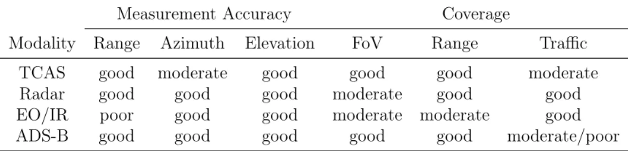
Further complicating the certification process of collision avoidance systems for unmanned aircraft is the diversity of their aircraft performance characteristics and sensor capabilities. Unmanned aircraft can range from under a pound to many tons with wildly varying flight dynamics. Several sensor modalities have been considered for supporting collision avoidance, including electro-optical/infrared (EO/IR), radar, TCAS, and Automatic Dependent Surveillance-Broadcast (ADS-B) [62, 42, 17, 119, 120, 82, 9]. As Table 1.1 illustrates, these sensor modalities vary in their

(17)

capabili-Table 1.1: Qualitative performance characteristics of various sensor modalities. FoV stands for field-of-view.

Measurement Accuracy Coverage

Modality Range Azimuth Elevation FoV Range Traffic TCAS good moderate good good good moderate Radar good good good moderate good good EO/IR poor good good moderate moderate good ADS-B good good good good good moderate/poor

ties. It would be very difficult to develop and certify a different collision avoidance system for every combination of sensor configuration and aircraft platform. Current efforts in the unmanned aircraft industry have focused on proprietary solutions for specific platforms and sensors, but a common system that would accommodate dif-ferent sensor configurations and flight characteristics would significantly reduce the cost of development and certification.

1.2

Challenges and Approach

In this document, we refer to the UAV that we control as own aircraft or ownship

and to the other aircraft involved in the encounter as intruder aircraft. Major chal-lenges of designing an autonomous collision avoidance system for own aircraft can be summarized as follows:

• We have a dynamical system and we need to take time into account in order to plan effective collison avoidance maneuvers.

• Most sensors have inherent measurement noise of different magnitudes depend-ing on the sensor type and specifications. Therefore the detected positions and the estimated velocities of intruder aircraft have observational uncertainties in them. Moreover, usually there is also uncertainty about the intention of the intruder aircraft. For example, a hostile intruder might attempt to collide with ownship, a risk-aversive intruder such as one following TCAS resolution

(18)

advi-sories might attempt to increase vertical separation between itself and ownship, or an intruder that is oblivious to ownship might follow its regular flight plan. Our algorithms need to account for various possible intentions. For this purpose, we will work with worst case assumptions and adopt parametric random walk models to cover a large spectrum from oblivious intruders1 _{to hostile intruders.}

• All aircraft, including ownship, have nonholonomic motion constraints. A non-holonomic system in physics and mathematics, is a system whose state depends on the path taken to achieve it [22], therefore planning maneuvers requires not just deciding where to be at a given time, but also how to get there. The implications of nonholonomicity are twofold: On one hand, we can use this in-formation to our advantage by limiting the locations that the intruder aircraft might occupy when we are estimating future states. On the other hand, we need to consider the limited mobility of ownship, too, and make sure that the planned escape maneuvers are feasible within the performance limits.

• Another very important challenge is the large size of the underlying state space of the collision avoidance problem. During the course of designing our algo-rithms and testing them using simulation software, we worked with up to 13 dimensional vectors to describe the state of a single aircraft. The components of our aircraft state vectors are listed in Table 1.2. The simplest collision avoid-ance problem involves two aircraft and hence the smallest true state space for an encounter has 26 dimensions. We also worked with realistic control com-mands shown in Table 1.3 and this necessitated the use of complex and realistic transition models in planning as well.

• As mentioned previously, there are many different types of sensor systems and UAVs which make designing collision avoidance systems difficult no matter whether we are hand-crafting individual algorithms for various different combi-nations of sensors and aircraft types or designing generic and parametric

algo-1 _{This is actually a reasonable assumption for the current state of the global airspace, because,}

due to high cost and weight, many small UAVs do not carry the necessary transponder hardware that would enable them to inform the intruder aircraft about their presence and/or flight plans.

(19)

Table 1.2: Aircraft state vector. Component Explanation v True airspeed in ft/s N Position, north in ft E Position, east in ft h Position, altitude in ft

ψ Orientation, yaw in rad

θ Orientation, pitch in rad

φ Orientation, roll in rad ˙

v Airspeed acceleration in ft/s2

p Roll rate in rad/s

q Pitch rate in rad/s

r Yaw rate in rad/s ˙

h Vertical rate in ft/s ¨

h Vertical acceleration in ft/s2

Table 1.3: Aircraft control command vector. The first component of the control command can be either a vertical rate or a vertical acceleration. The simulation software that we used to test our algorithms is capable of working with both types of control commands.

Component Explanation ˙

h or ¨h Vertical rate in ft/s or vertical acceleration in ft/s2

˙

ψ Turn rate in rad/s

a Airspeed acceleration in ft/s2

rithms that can accomodate different sensor modalities and flight characteris-tics.

Having presented the major challenges, our approach to the problem will consist of the following key components:

Our first objective will be to answer the challenges stated above. Our algorithms will plan dynamical collision avoidance maneuvers. We will try to account for uncer-tainties in observations of intruder positions, velocities and intentions. The escape maneuvers will be feasible, i.e., ownship will be able to execute the planned maneuvers within its performance limits. In order to handle large problem space dimensionality, we will pick only the most relevant dimensions and come up with new representations

(20)

that capture and summarize important aspects of the problem that are sufficient for collision avoidance planning. We will design our algorithms to be parametric such that they will accomodate different sensor modalities and aircraft flight characteristics.

We will be working with realistic aircraft state vectors and control commands. We will also aim for designing algorithms that will work in real time such that they are suitable for deployment on real platforms.

There are avionic transponder systems that allow an aircraft to transmit and receive flight plans, intentions and planned escape maneuvers. If all aircraft in an encounter were equipped with such transponders, it would be possible and probably more effective to plan collision avoidance maneuvers for all aircraft at once. Such maneuvers are called coordinated escape maneuvers and the execution of a coordi-nated maneuver requires strict cooperation from all involved. In this work, we will assume that there is no cooperation between aircraft and we are planning only for ownship. However, some of our algorithms are also adequate for planning coordinated maneuvers and we will briefly make a note of them in respective sections.

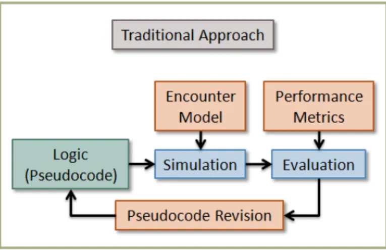
Instead of the traditional way that collision avoidance algorithms have been de-signed, we will use a model-based approach to facilitate the design of algorithms that accomodate different sensors and flight dynamics. The traditional approach and the model-based approach are depicted and described in Figures 1-1 and 1-2, respec-tively. Briefly, a model-based design system takes as input models of flight dynamics, intruder behavior, and sensor characteristics, and attempts to optimize the avoid-ance strategy so that a predefined cost function is minimized. The cost function can take into account competing objectives, such as flight plan adherence and avoiding collision.

One way to formulate a problem involving the optimal control of a stochastic system is as a Markov Decision Process (MDP) [56, 110], or more generally as a Par-tially Observable Markov Decision Process (POMDP) to also account for observation uncertainty [3, 124, 128, 25, 50, 23, 64, 122]. POMDPs have been studied in the operations research and artificial intelligence communities, but only in the past few years have generic POMDP solution methods been developed that can approximately

(21)

Figure 1-1: Traditional approach to designing collision avoidance algorithms. The input to the design process is the initial collision avoidance logic which is usually in the form of pseudocode. Human effort is spent on designing encounter models, developing performance metrics and revising collision avoidance logic. Simulations and evaluations are usually performed by computers. The design process consists of iterative improvements to the logic until desired performance is achieved. The output of the process is the improved collision avoidance logic.

Figure 1-2: Model-based approach to designing collision avoidance algorithms. The input to the design process are encounter models and performance metrics, and human effort is spent on designing the input only. Computers perform the optimizations and it is desirable to do as much offline computation as possible. The design process ends as soon as the optimizations are completed. The output of the process is the optimized logic which might not be in a form that is easily interpreted by humans. For some of our algorithms that will be presented later, the output logic is a cryptic lookup table of high-dimensional vectors that is meant to be executed by special software.

(22)

solve2 _{problems with moderate to large state spaces in reasonable time (for example}

the solvers we used [125, 80]). In this work, as our first approach, we will investigate the feasibility of applying state-of-the-art MDP and POMDP solution methods to the collision avoidance problem. Due to the fact that large-sized model spaces usu-ally have a negative impact on the time required for solution and the effectiveness of the policy computed by MDP/POMDP solvers, we will limit our collision avoidance strategies to vertical evasion maneuvers only and compare our results against some baseline collision avoidance systems including TCAS, which also assists the pilots to do vertical-only evasive maneuvers. The experiments we will present in this docu-ment show that we can actually model collision avoidance systems using MDPs, and such systems perform very well in terms of both reducing the risk of collision and having very little deviations from the flight plan at the same time, especially with sensors that precisely locate intruder aircraft. We will also present experiments with POMDP models built for sensors with limited observation capabilities that demon-strate how we can still achieve low risk of collision by maneuvering a little more in order to counterbalance the limitations in observability of intruder aircraft.

The MDP and POMDP models we implemented in this study require working with finite number of states, control commands and sensor observations. Therefore, every input, output, and most intermediate results need to be chosen from discretized sets of values. Since the state space for collision avoidance problem is very high-dimensional and even the most powerful MDP/POMDP solvers cannot currently deal with very large sets yet, it is not possible to have nice and fine-grained discretizations of input and output spaces. There are also other negative effects of discretization that reduce the effectiveness of our collision avoidance algorithms as we will point out in the following sections. As a result of these observations about the MDP and POMDP models, our last objective will be set for investigating if we could design a hybrid collision avoidance system that would not require discretization of every data space and that could work on a mixture of continuous and discretized spaces as necessary.

2_{Approximate POMDP solution methods typically return solutions with bounded regret. Regret}

(23)

For this purpose, we implemented a technique that we call the path-modification or

spaghetti method, which basically takes as input the estimated flight plans of all aircraft in an encounter, and outputs an optimized flight plan for ownship that tries to avoid risk of collision, not deviate much from the original flight plan, and minimize maneuvering at the same time. The experiments with algorithms based on the path-modification technique that we will present in this document show the feasibility of using this hybrid method to perform full 3-D evasion maneuvers (planning with full aircraft control commands as shown in Table 1.3, rather than planning for vertical-only maneuvers as we do with MDP/POMDP models).

1.3

Organization of the Thesis

The remainder of this document is organized as follows: In Chapter 2, we present a review of the MDP/POMDP framework that will be the basis for the first set of our algorithms, and a summary of previous work on collision avoidance techniques. Then we describe the parametric aircraft model, the sensor models, and the sim-ulation and evaluation framework that we will work with. In Chapter 3, we build MDP/POMDP based collision avoidance systems with increasing complexities for the cases of perfect, noisy and limited field-of-view sensing, respectively. Chapter 4 de-scribes the path-modification technique and two algorithms based on that technique for planning 3-D escape maneuvers. Finally, Chapter 5 delivers concluding remarks and recommendations for future research.

(24)

(25)

Chapter 2

Background

In this chapter, we will first present a brief review of MDP/POMDP framework. Then we will look at major approaches that have been applied to aircraft collision avoidance. The review of major approaches will be followed by an overview of the aircraft and sensor models that we implemented for use in our collision avoidance algorithms. Finally, we will introduce the simulation and evaluation framework.

2.1

Review of MDPs and POMDPs

An MDP is a stochastic process where the state of the system changes probabilistically according to the current state and action. MDPs assume that the state is fully observable. POMDPs remove that assumption and replace it with a stochastic model for observations, and hence they have more expressive power. We will briefly review POMDPs in this section.

The solution to a POMDP is a policy, or way of behaving, that selects actions in a way that takes into account both the current uncertainty about the underlying state of the system (e.g., exact relative position of the intruder aircraft), as well as future uncertainty about how the system state will evolve (e.g., what kinds of maneuvers the intruder aircraft will make), by aiming to maximize the expected accumulation of some predefined reward or minimize the expected accumulation of some predefined cost [64]. Due to their rich descriptive power, POMDPs have found many uses in

(26)

computer science and robotics applications such as robust mobile robot navigation [123], machine vision [6, 31], robust dialogue management [118, 55], autonomous helicopter control [4, 103], and high-level robot control [107], as well as in many other areas like machine maintenance [110], network troubleshooting [133], medical diagnosis [49], and preference elicitation [18]. Cassandra provides a comprehensive survey of applications utilizing POMDPs [24].

Several formulations of POMDPs have been studied in the literature, but this work focuses on the discrete-time formulation with discrete state and action spaces. We briefly present below a POMDP formulation and discuss solution techniques.

2.1.1

Formulation

In this document, we use S to represent the state space, A to represent the action space, and Ω to represent the observation space, all assumed discrete. The state-transition function T ∶ S × A → Π(S) determines the probability distribution over the next states given the current state and action taken. The probability of tran-sitioning to state s′ after taking action a from state s is written T(s, a, s′). The

observation function O ∶ S × A →Π(Ω) determines the probability distribution over the observations received after taking some action resulting in states′. The probabil-ity of receiving observation o after taking action a and landing in state s′ is written

O(s′, a, o).

In general, the initial state is unknown. The uncertainty in the initial state is represented by a probability distribution b0 ∶ S →R, where the probability of starting

in statesis writtenb0(s). Since the true state is not directly observable in POMDPs,

the states are called belief-states, and similar to the initial state, they consist of probability distributions over the state space;S →_R. The space of all possible belief-states is denoted B. The belief-state b is initialized to b0 and updated with each

(27)

taken resulting in an observation o, the new belief-state b′ is given by b′(s) = Pr(s′∣o, a, b) ∝ Pr(o∣s′, a, b)Pr(s′∣a, b) = Pr(o∣s′, a) ∑ s∈S T(s, a, s′)b(s) = O(s′, a, o) ∑ s∈S T(s, a, s′)b(s).

The belief-update process is often referred to as state estimation.

Given the current belief-state, the objective is to chose an action that maximizes the expected discounted return. The discounted return for a sequence of states st and

actions at is given by ∞ ∑ t=0 γt_R(_s t, at),

where γ ∈ [0,1) is a discount factor and R ∶ S × A →_R is the reward function. The reward for taking action a from states is written R(s, a).

The solution to a POMDP is a policy π ∶ B → A that specifies which action maximizes the expected discounted reward given a belief-state. It is known that optimal policies can be represented as a collection of α-vectors, denoted Γ. Each

α-vector is a vector consisting of ∣S∣ components and is associated with a particular action. The expected discounted return when starting with belief b is

V(b) =max

α∈Γ (α⋅b),

where α⋅b is the inner product of an α-vector with a vector representation of the belief-state. The function V is known as the value function. The policy evaluated at belief-state b is the action associated with the α-vector that maximizes the inner product.

(28)

2.1.2

Solution Methods

Finding the collection of α-vectors that represents the optimal policy can be chal-lenging, even for relatively small problems. A variety of exact solution methods can be found in the literature [127, 124, 128, 48, 98, 113], but generally these methods do not scale well to large problems. Approximate solution methods generally scale much better and many of them provide bounds on theregret for the policies they find. The regret of a policy π is the difference between the expected discounted return start-ing at b0 when following π and the expected discounted return starting at b0 when

following an optimal policy π∗.

Point-based methods for finding approximate solutions to POMDPs (for example, Point-Based Value Iteration, PBVI [106]) have received attention in recent years be-cause of their ability to solve problems that are orders of magnitude larger than was previously possible. Point-based methods involve sampling from the belief space B. The more successful point-based methods focus the sampling on belief-states. In this work we initially used solvers based on Heuristic Search Value Iteration (HSVI2) al-gorithm [125, 126]. We later switched to a solver that uses Successive Approximations of the Reachable Space under Optimal Policies (SARSOP) algorithm [80, 58, 57] as it performed better on our problems. An implementation of SARSOP is publicly avail-able1 _{and we were able to use the software without any modification. SARSOP takes}

as input a textual representation2 _{of a POMDP, including} _γ_, _b

0,R,T, andO. When

the regret bounds fall below some preset value or the user interrupts the solution process, SARSOP outputs a policy file represented as a collection of α-vectors.

Crucially, although it may require considerable computation to find a near-optimal policy, this work is done offline. Once a policy has been computed, it can be executed very efficiently online. In the course of this work we have developed a new algorith-mic technique to make the execution process even more efficient, making it entirely suitable for execution online, in real time, on an aircraft.

1 _M2_{AP Research Group at NUS,}_{POMDP Planning}_,

http://motion.comp.nus.edu.sg/projects/pomdp/pomdp.html (August 2010).

2 _{The format of the input is the same as the one described by Anthony R. Cassandra,} _Input

(29)

Although our MDP/POMDP based collision avoidance algorithms have focused on finding α-vectors offline, there are other approaches to finding and representing policies. Online approaches decide what action to execute by searching only from the current belief-state, instead of trying to find a comprehensive policy that is optimal for all belief-states [117]. From the current belief-state, these methods explore differ-ent action sequences up to some horizon and then select the sequence that results in the largest expected discounted return. Computing the expected discounted return for an action sequence involves updating the belief-state based on hypothetical mea-surements obtained with each state transition. One concern with an online method that involves sampling might be the nondeterminism of the resulting behavior.

2.2

Previous Work

Collision avoidance is a fundamental part of motion planning, and hence there are many different approaches from ad hoc solutions to well-established methods. In this section, we will present a summary of major techniques that have been used for collision avoidance and discuss their advantages and disadvantages.

2.2.1

POMDPs and Dynamic Programming

Due to the large size and the continuous nature of the state, observation and action spaces in most collision avoidance tasks, classical POMDPs operating on discretized sets have been difficult to apply to realistic collision avoidance scenarios. To the best of our knowledge, our MDP/POMDP based algorithms are some of the first examples of application of the original POMDP formulation to a realistic UAV collision avoid-ance problem, where the models monitor a very large airspace and choose realistic control commands for maintaining a flight plan, collision avoidance, and information gathering. We were able to use the classical framework by choosing compact rep-resentations and carefully designing small state, action and observation spaces that contain sufficient information. This is a major difference of our models from the ones described below: Almost all of the following techniques differ in certain ways from

(30)

the discrete-time POMDP formulation in order to increase the size of the models that could be handled and/or work with continuous spaces.

One heuristic that is likely to be necessary in order to feasibly employ the discrete-time formulation for even larger problems is to hierarchically decompose the planning task [52, 83, 8]. With this approach, domain-specific knowledge could be leveraged to perform planning in macro and micro scales that are managed by different layers of the hierarchical planner.

If we assume that the world state that is ‘most likely’ in the current belief-state is in fact true, then we can take the optimal action for the state in the MDP that underlies the POMDP. Similar simplifications include Q-MDP [88] and value-function approximations [51]. One important problem with ignoring uncertainty about cur-rent state and assuming full observability is the loss of system’s desire to explicitly take actions to reduce uncertainty. Platt et al. [109] employ the key idea of plan-ning directly in belief-space, determinizing the dynamics by using the most-likely observation, and demonstrate a replanning approach to overcome that problem us-ing optimization schemes like linear quadratic regulation [130], direct transcription [38] (solving control problems by treating them as optimization, based on nonlinear optimization methods [12]), and other standard planning/control techniques.

POMDPs with continuous state spaces, leveraging hybrid-linear system dynamics, have been developed and applied to UAV collision avoidance simulations by Brunskill et al. [20, 21]. In their study, a formal analysis with bounds on the quality of resulting solutions has also been presented. Erez and Smart take this approach further, and work with all continuous state, observation and action spaces [39]. They parametrize the belief-state as a mixture of Gaussians and use Differential Dynamic Programming [61] for local optimization. Such local optimization provides no guarantees of global optimality, but it accommodates domains that are much larger than those that could be solved feasibly by state-of-the-art solvers that require the discretization of state, observation and action spaces.

Wolf and Kochenderfer propose an online POMDP approach to collision avoidance [142, 143]. Online planning has the advantage of starting from current state and

(31)

searching only the reachable states instead of having to come up with a universal policy for all possible initial states. They utilize continuous state and observation spaces and a finite action space in their formulation, and they introduce sample-based representation of state uncertainty [135] to an existing algorithm called Real-Time Belief Space Search [105].

Kochenderfer et al. use a dynamic programming approach to generate optimized TCAS logic [71, 74]. They also provide guidance in justification of collision avoidance logic that is automatically generated by dynamic programming based solvers, which will be a very important issue as more complex solvers are being developed and used in optimizations. They extend their framework later to include more sophisticated actions, motion estimations in 3 dimensions, probabilistic pilot response, noisy sensor measurements, coordinated resolution maneuvers and multiple intruder scenarios [73].

2.2.2

Potential Field Methods

The artificial potential field approaches have been widely used in robot navigation planning since their introduction [70, 67, 68, 69, 84]. They have also been applied to aircraft collision avoidance [36, 37]. Typically, the problem is set up such that the target location exerts attractive virtual forces and the obstacles exert repulsive virtual forces. The controller then computes and commands to step in the direction of the net resultant force acting on own agent.

Potential field methods are very fast and they allow implementations of real-time planners very easily, but they have fundamental problems [76]. Most important limitations from the point of view of application to aircraft collision avoidance include the following:

• Potential field methods are prone to local minima problems. The attractive and repulsive forces might cancel each other and lead to a zero resultant force. There is a need to have higher-level planners to escape from such traps.

• Nonholonomic motion constraints might prevent the agent from being able to move immediately in the direction of the resultant force. This is an important

(32)

limitation, but a technique used by pilots for aircraft formation [40] might be utilized as a heuristic to alleviate the problem: Positioning is decomposed into fore-aft corrections (done by adjusting speed only) and side-side corrections (done by adjusting heading only) which can be applied independently. Balch and Arkin demonstrate the use of this type of corrections to navigate unmanned ground vehicles with nonholonomic constraints [5].

• Potential field methods can work well for slow-moving robots, but it is difficult to fully consider wide range of aircraft dynamics (including probabilistic dynamics of intruder aircraft) when they are applied to aircraft collision avoidance. Large virtual forces are necessary for repelling fast incoming traffic, but with slower intruders, this will cause unnecessary deviation from planned flight trajectories.

• Most importantly, uncertainty in control or observation might be challenging to model with sufficient fidelity for aircraft collision avoidance. It might be possible to account for uncertainties by increasing protected volumes around all aircraft (in the sense of configuration-space based spatial planning [92, 90, 91]), but in the last-minute collision avoidance context, it is not enough due to the short encounter time frame and the catastrophic nature of collision.

Charifa and Bikdash provide a comparison of several variants of artificial potential field approaches with emphasis on the quality of the path geometry, and velocity and acceleration profiles [28].

2.2.3

Sampling-Based Motion Planning

Sampling-based planning algorithms and especially Rapidly-Exploring Random Trees (RRTs) have been widely used because they tend to cover the search space more quickly than a random walk or other types of structured searches [7, 26, 66, 94, 59, 63, 85]. They are usually adequate for building real-time planners (for example, they have been applied to autonomous urban driving [81]).

RRTs generate random samples to explore the configuration space of the agent and they try to find a solution by extending and finally connecting one or more trees

(33)

rooted at the origin and at the destination configurations. Similar to our algorithms that we will present later, RRTs work very well with nonholonomic agents as they plan in configuration space.

Some fundamental issues with sampling have received increased attention recently [87], and further improvements have been suggested [86]. As a general condition, sampling-based methods make no guarantee of optimality of the found solution, and consideration of uncertainty in this framework is not yet mature enough to be fully feasible in the airborne collision avoidance problem domain.

2.2.4

Geometric Optimization

Bilimoria introduced a 2-D conflict resolution algorithm in horizontal plane using ge-ometric computations [14]. Conflict predictions are based on straight-line projections using positions and assuming constant velocities. Computed resolutions consist of minimal changes in velocity to avoid a predefined circular protected airspace around intruder aircraft. Dowek et al. generalized this analytical approach to 3-D with cylin-ders replacing the circular protected zones, and full aircraft control commands rather than lateral-only maneuvers [45].

Geometric solutions to collision avoidance have the unique advantage of being extremely fast and very easily verifiable and validatable, but precautions such as adjusting the protected airspace sizes and breaking the constant velocity assumptions should be taken in order to account for uncertainties in sensing and intruder intent, and unexpected intruder dynamics. Another disadvantage of geometric planning is that, it might not be easy to scale up the approach to avert multiple threat. When there are multiple intruders, there seems to be three ways of approaching the problem, with each one having its associated difficulties:

• Protected airspaces around all intruder aircraft might be merged into a big protected zone (as in building a convex hull) that is to be avoided by geometric computations. There are basically three problems with this approach: First; the resulting protected zone could be very big and cannot be avoided within

(34)

the performance limits of ownship. Second; individual protected airspaces are projections of estimations through time, and hence they might shift around and/or shrink/grow in size as estimated positions and velocities of intruders are updated with each new observation. Third; the optimal (safest) trajectory that could be followed by ownship might fall within the convex hull, which will never be considered by the solver.

• Pairwise solutions against each individual intruder could be computed and heuristics could be developed to merge them into a global solution, but fun-damental problems with this approach is described by Kuchar and Yang [79].

• A full 3-D global planning that aims to avoid each and every protected airspace is actually the optimal approach, but this turns the planning into a 3-D version of TCAS (which computes just vertical-only maneuvers and is already very complex).

2.2.5

Policy Search Methods

Given a parametric representation of a collision avoidance policy, a local search method known as policy gradient [102] can be used to search the parameter space for an optimal setting that minimizes the expected cost of following that policy. In this method, the state space does not need to be discrete and the policy could be represented very flexibly (for example, it can be a set of parametrized controls to be applied sequentially, or a functional pseudocode such as TCAS, or it can even be in the form of a neural network [53, 54]). Sample applications of policy search include autonomous helicopter flight [104] and aircraft collision avoidance planning [65, 140]. Aside from its benefits, policy search methods suffer from local minima problems as do all local optimization techniques. Also, the design of the parametric representation of a policy requires deep domain-specific knowledge, insight into problem structure and engineering judgment.

(35)

2.2.6

Mixed Integer Linear Programming

Spacecraft and aircraft trajectory optimization including collision avoidance can be expressed as a list of linear constraints involving integer and continuous variables, known as a mixed-integer linear program (MILP) [10, 139], which can then be solved using efficient commercial software [108]. Richards and How demonstrate a single aircraft collision avoidance application, and then generalize their approach to allow for visiting a set of waypoints in a given order, and also handling multiple aircraft planning [115]. Luders applies MILP formulation with non-uniform timesteps between target waypoints, and plans a detailed short-term trajectory and a coarse long-term trajectory for own aircraft [93].

As in the geometric optimization approaches, there is usually a protected airspace set up around each aircraft in the MILP formulations. The stochasticity that stems from uncertainties in observations, intruder intent, and unexpected aircraft dynamics could be handled by increasing the sizes of protected airspaces.

MILP formulations using a set of target waypoints that need to be visited in a certain order have a strong structural resemblance to our path-modification based collision avoidance models. An advantage of the MILP formulation over our mod-els is its ability to plan with non-uniform timesteps between waypoints, since our waypoints are currently fixed in time. However, an important difference between the two approaches lies in the problem statement and the solver structure. The MILP approach requires all aspects of the problem (dynamics, ordering of all waypoints in time, and collision avoidance geometry) to be specified as a carefully designed and a usually long list of many linear constraints, and then the solver’s task is basically to find a solution that satisfies all of those constraints simultaneously. The path-modification technique requires less information (just the aircraft dynamics and cost formulation) in the formulation stage, and the solver performs iterative optimization of an initial solution (planned flight).

(36)

Figure 2-1: Global Hawk.

2.2.7

Other Approaches

Other approaches to aircraft collision avoidance domain such as evolutionary algo-rithms [11] and nonlinear programming [112] can be found in the literature. Carlos et al. present a survey of a family of high performance controllers that is referred to as Model Predictive Control (MPC) [43], and examine their performances, advantages, and their application to nonlinear systems. Fujimura provides detailed general back-ground information on motion planning in dynamic environments against stationary and dynamic obstacles [41]. Kuchar and Yang present an assessment of 68 air traffic conflict detection and resolution methods in their survey [79]. Kuchar also describes a unified methodology for the evaluation of hazard alerting systems in his thesis [77] that could be used in performance evaluation of miscellaneous and/or new future techniques that do not fit in any of the categories we have reviewed.

2.3

Aircraft and Sensor Models

The aircraft model we developed for our collision avoidance systems is parametric and can be modified to mimic different types of aircraft. In our implementation, parameter values are based on Global Hawk, an unmanned aerial vehicle used by the United States Air Force as a surveillance aircraft, shown in Figure 2-1.

(37)

Table 2.1: Global Hawk performance limits. Maximum velocity 180 kts Minimum velocity 100 kts Maximum climb rate 3500 fpm Maximum descent rate 4000 fpm Maximum bank angle 35 deg Maximum bank rate 8 deg/s Maximum pitch rate 2 deg/s Maximum turn rate 2.5 deg/s

models use a subset of these values; namely, maximum and minimum velocities, maximum climb/descent rates and turn rate. Our evaluation environment makes full use of them during encounter simulation.

Before describing our sensor models, let us introduce four coordinate systems shown in Figure 2-2 that we will refer to from time to time in the rest of this document:

• Global Coordinate System (GCS): This coordinate system is also known as the Earth Coordinate System. The origin is an arbitrary point chosen by the model simulation and evaluation framework. Positive x is east, positive y

is north, and positivez is altitude.

• Local Coordinate System (LCS): The origin of LCS is ownship center of mass (i.e., LCS is anegocentric coordinate system). Positivexis in the direction of the right wing, positive y is the direction of the nose, and positive z is upwards.

• Auxiliary Coordinate System (ACS): This is also anegocentric coordinate system whose x-y-z axes are aligned with the east-north-altitude axes of GCS, respectively.

• Relative Coordinate System (RCS): This is another egocentric coordi-nate system which is obtained by rotating ACS around its z axis until the

y-z plane contains (intersects with) intruder aircraft center of mass. RCS is a 2-dimensional coordinate system. The x and y axes of RCS are the y and

(38)

Global Coordinate System Local Coordinate System

Auxiliary Coordinate System Relative Coordinate System Figure 2-2: Coordinate systems.

(39)

RCS (viewed from above) Projection Plane

Figure 2-3: Relative position of the intruder aircraft can naturally be represented by a point on Projection Plane.

z axes of the rotated ACS, respectively. The RCS is also referred to as the projection plane due to the fact that the vertical and horizontal distances to intruder aircraft can both be naturally projected on RCS to obtain a compact representation of aircraft separation as shown in Figure 2-3.

Input to our collision avoidance systems may come from various sensors with different characteristics and sensing ranges (usually expressed by radii in nautical miles, NM) onboard the UAV. We developed four detailed sensor models that are capable of simulating following types of erroneous measurements and noise:

• False positive measurements: We may detect an intruder when, in fact, there is no intruder aircraft in the sensor range (for example, a bird in sensing range might cause false positive measurements).

• False negative measurements: We may fail to detect an intruder when one is present in the sensor range.

• Measurement errors: We may detect the intruder aircraft in a position or at an angle that is not correct.

The probabilities of false positive and false negative measurements (pfp and pfn) are usually specific to different sensor hardware, and the measurement errors are com-puted according to realistic error models. In addition to false positive and false

(40)

negative measurements, one can think of a third type of false measurement: We may detect a different intruder (for example, a bird or some other random measurement) when there is a real intruder aircraft in sensor range. We excluded this case in our sensor models with the following assumptions:

• Sensors are tested for and free of this type of fault.

• If there are both a plane and a bird in the sensor range (and assuming that this is not a case of a false negative measurement), sensor will detect the plane since it is much bigger than a bird.

The four sensor models studied in this research are as follows:

1. Perfect sensor: This is a hypothetical omnidirectional sensor with no noise and no false positive/negative detections (pfp = pfn = 0). The sensor reading consists of east, north and altitude coordinates of intruder aircraft in GCS (it can be thought of as providing an abstract resemblance to the functionality of an ADS-B sensor). With this sensor, it is possible to localize intruder aircraft to an exact point in both GCS and LCS.

2. TCAS sensor: This is a model of the actual TCAS sensor [119]. It is based on listening to transponder replies from nearby aircraft and is omnidirectional. It providesbearing in LCS,altitude in GCS, andrange (the line-of-sight distance between ownship and intruder aircraft, also referred to as slant range). The error in range measurement is Gaussian with zero mean and 50 ft standard deviation. The error inbearing estimate is Gaussian with zero mean and 10 deg standard deviation. The altitude of intruder aircraft is measured with 25 ft quantization. There is also an altimetry error bias that remains constant during an encounter with an intruder aircraft, and is Laplacian with zero mean and 40 ft scale. Probability density function for the Laplace distribution is shown in Figure 2-4. In the TCAS sensor model, pfp = 0 (since detection is based on broadcast signals) and pfn =0.01. With a noiseless TCAS sensor, intruder

(41)

Figure 2-4: Probability density function for the Laplace distribution (location = 0, scale = 40).

model, the region that the intruder could be residing in has approximately the shape of a distorted truncated spherical cone.

3. Radar sensor: Our radar sensor model has a limited field-of-view (FoV),

±15 deg elevation and ±110 azimuth. It provides bearing and elevation read-ings in LCS, and range and range rate information. As with TCAS, the error in the range measurement is Gaussian with zero mean and 50 ft standard de-viation. Range rate error is Gaussian with zero mean and 10 ft/s standard deviation. The error in the bearing estimate is Gaussian with zero mean and 10 deg standard deviation. Elevation error estimate is Gaussian with zero mean and 1 deg standard deviation. For the radar sensor, pfp = pfn =0.01. Intruder

aircraft can be localized approximately into a distorted truncated spherical cone in LCS.

4. Electro-optical/infrared (EO/IR) sensor: Our EO/IR sensor model is very similar to the radar sensor with less angular measurement noise and without a

range reading. It has a limited FoV,±15 deg elevation and±110 azimuth. Sensor reading consists of bearing and elevation angles in LCS, and line-of-sight rate

information. Error in both angular measurements is Gaussian with zero mean and 0.5 deg standard deviation. Line-of-sight rate error is Gaussian with zero mean and 0.5 deg/s standard deviation. For the EO/IR sensor, pfp =pfn =0.01.

(42)

Figure 2-5: Comparison of sensing regions. The figure on the left shows omnidi-rectional sensing region, the figure at the center shows limited field-of-view sensing region, and the figure on the right shows both sensing regions overlapped for better comparison.

Intruder aircraft can be localized approximately into a distorted spherical cone in LCS.

Figure 2-5 shows a comparison of the omnidirectional and limited field-of-view sensing regions. Complete list of sensor parameter values are given in Table 2.2.

2.4

Simulation and Evaluation Framework

The performance of our collision avoidance systems were evaluated using a simulation framework called Collision Avoidance System Safety Assessment Tool (CASSATT). The framework was developed for assisting prior TCAS studies [121] and evaluating sense-and-avoid systems for unmanned aircraft [15] at Lincoln Laboratory at Mas-sachusetts Institute of Technology.

We used an encounter model derived from 9 months of national radar data [75] to generate 15,000 scripted encounters between pairs of aircraft and allowed our col-lision avoidance systems to control one of the aircraft. For comparison, we evaluated the performance of other collision avoidance systems to baseline performance. This section describes our simulation and evaluation process.

(43)

Table 2.2: Complete list of sensor parameter values.

Perfect

Range 5 NM

False positive measurement probability 0.00 False negative measurement probability 0.00

TCAS

Range 5 NM

Altitude quantization 25 ft Range error standard deviation 50 ft Bearing error standard deviation 10 deg Altimetry error scale 40 False positive measurement probability 0.00 False negative measurement probability 0.01

Radar

Range 5 NM

Minimum azimuth −110 deg

Maximum azimuth 110 deg

Minimum elevation −15 deg Maximum elevation 15 deg Range error standard deviation 50 ft Bearing error standard deviation 1 deg Elevation error standard deviation 1 deg Range rate error standard deviation 10 ft/s False positive measurement probability 0.01 False negative measurement probability 0.01

EO/IR

Range 5 NM

Minimum azimuth −110 deg

Maximum azimuth 110 deg

Minimum elevation −15 deg Maximum elevation 15 deg Bearing error standard deviation 0.5 deg Elevation error standard deviation 0.5 deg Line-of-sight rate error standard deviation 0.5 deg/s False positive measurement probability 0.01

(44)

2.4.1

Simulation Framework

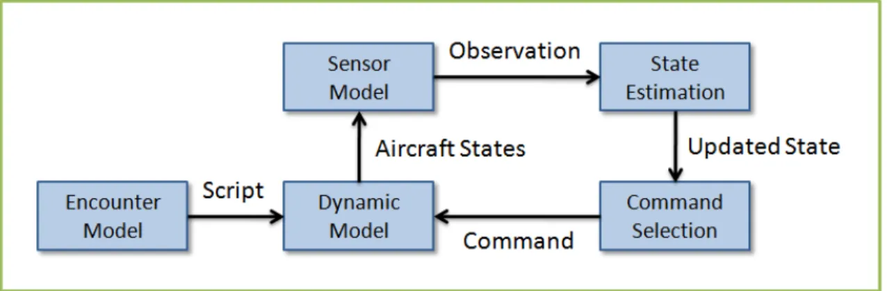
CASSATT framework was built in Matlab and Simulink and has been compiled into native code using Real-Time Workshop. The framework was designed to be modular to allow different collision avoidance systems and sensor models to be easily incorpo-rated. As part of this work, we extended CASSATT to allow communication with the collision avoidance system over a TCP/IP socket connection. This extension allows changes to be made to the collision avoidance system without having to recompile the remainder of the CASSATT system. The collision avoidance system runs as a server to which CASSATT connects as a client. Socket communication also allows CASSATT to run on a different machine from the collision avoidance system; for our experimentation however, we always ran the collision avoidance system on the same machine as CASSATT.

Figure 2-6 provides an overview of the simulation framework. An encounter model is used to generate initial conditions and scripted maneuvers for both aircraft involved in the encounter. These initial conditions and scripts are fed into a 6 degree-of-freedom, point-mass dynamic model. The sensor model takes as input the current state from the dynamic model and produces an observation, or sensor measurement. The state estimation process updates the internal state estimate of the collision avoid-ance system based on the observation. Then the collision avoidavoid-ance system selects the control command that minimizes some cost depending on the algorithm used. Finally, the dynamic model updates the simulation state, and the process continues until the end of the encounter.

Encounter Model

Initial conditions and scripted maneuvers for both aircraft are generated by an en-counter model. The initial condition for each aircraft is basically an aircraft state vector that was introduced before in Table 1.2. A scripted maneuver consists of a set of aircraft control commands described in Table 1.3 and the associated times that each command is to be applied during the encounter. In the simulations, scripted

(45)

maneu-Figure 2-6: Simulation framework.

vers represent the Air Traffic Control (ATC) commands to each aircraft. The intruder aircraft always follows its script for the whole duration of the encounter. Ownship, however, is allowed to choose to follow the ATC commands or apply different control commands selected by the collision avoidance system.

We used a recently developed encounter model derived from 9 months of radar data from over 120 sensors [75]. A dynamic Bayesian network [101] representing the behavior of the aircraft was learned [44] from actual encounters extracted from the dataset. Generating new encounters for use in Monte Carlo analysis involves sampling from this dynamic Bayesian network.

Dynamic Model

Aircraft dynamics are represented using a tunable 6 degree-of-freedom, point-mass dynamic model, which includes aircraft transient response characteristics and perfor-mance limits such as maximum pitch rate or bank angle. The aircraft flight trajecto-ries are defined by an encounter model and based on vertical rate, aircraft turn rate, and airspeed acceleration. These control values may change every tenth of a second.

Sensor Model

The sensor simulation module takes as input the raw (non-noisy) coordinates of both aircraft in GCS. First, the position of the intruder aircraft is computed (relative to ownship) in LCS. These intermediate coordinates are then converted into a simulated

(46)

sensor reading by adding noise according to the respective sensor’s error model as described in Section 2.3. The pseudocode for the simulation of sensor readings is provided as Algorithm 1 in Appendix A. If we are evaluating a POMDP collision avoidance system (rather than a baseline or a path-modification based system) a final step takes the sensor reading, and generates an observation o∈Ω to be used in state estimation.

State Estimation

The state estimation module estimates the current state based on the measurement from the sensor. For path-modification based collision avoidance models, internal state is updated according to the sensor reading. For an MDP model, the current state is observed directly, and for a POMDP model, the belief-state is updated. Updating the belief-state usually requires iterating over large tables, and computing and normalizing probability values. Therefore, an important practical aspect of the belief-state update process is the overall computation time. This becomes even more crucial in real-time applications such as our collision avoidance systems. In this work, we developed a method that significantly reduces the computation time of the belief-state update process by merging the transition and observation models into a single look-up table that is generated offline and stored using sparse data structures [131, 132] (described in Appendix C). With this method, we have experienced belief-state updates that are 100 to 1000 times faster than a na¨ıve implementation.

Command Selection

The path-modification based algorithms pick a command from the set of available commands by computing various cost terms and trying to minimize the expected cost. For MDP/POMDP based collision avoidance algorithms, command selection is done by evaluating the policy to compute the action, i.e. to choose the control command, to be executed. For MDP models, policy evaluation is carried out by simply referencing theMDP policy, which is basically a table that has an actiona∈ A

(47)

α-vector that maximizes the expected long-term reward given the current belief-state, as described in Section 2.1.1. The output is the action associated with thatα-vector. As we mentioned in Section 2.1.2, there are powerful solvers available for POMDP formulations such as SARSOP and HSVI2 solvers, and the solutions generated by these solvers are called policies. Computing a policy with very tight regret bounds usually takes a very long time, sometimes on the order of hours or days, especially for large POMDPs such as the ones we use in our algorithms. Therefore, most POMDP solvers usually generate a simple solution first (probably with loose regret bounds), and iteratively improve that solution allowing the user to stop the process when tight-enough bounds are reached. Iterative improvement allows some solvers to work up to a given time limit or until a specified bound is reached. Policies are usually computed offline.

Policy evaluation is a process that takes two inputs and generates a single output. The inputs are a belief-state and a policy. The output is the action that we should take in order to maximize the expected long-term reward. We sometimes refer to the output as thebest action.

The space of all belief-states for a given POMDP formulation is called the belief simplex. An optimal policy maps belief-states (which correspond to points in the belief simplex) to actions that maximize expected long-term reward. Due to the continuous nature of the belief simplex, policies are usually represented as a collection of regions of belief simplex, and the associated actions that should be taken when the given belief-state falls inside those regions. More specifically, a practical implementation of a policy consists of a set of α-vectors with an action associated with each α-vector. An α-vector serves two purposes:

1. The maximum cardinality for anα-vector is the number of states in the POMDP formulation. Usually, most of the α-vectors of a policy contain less than the maximum number of entries. The entries that are present in an α-vector deter-mine the region of the belief simplex this α-vector is applicable to. Usually a policy contains a singleα-vector or a small number of α-vectors with maximum cardinality. These vectors are applicable to all of the belief simplex (all possible

(48)

belief-states). The rest of theα-vectors in the policy are specialized to different sub-regions. Note that different sub-regions might overlap, and they are not required to cover the belief simplex. Also, a policy may contain more than one

α-vectors that are all applicable to the same region.

2. The inner product of an α-vector and the belief-state yields the expected long-term reward in case of taking the action associated with that α-vector.

As a result, the algorithm for policy evaluation takes the following form:

• Determine the applicable α-vectors for the given belief-state.

• Compute expected long-term rewards by taking inner products of all applicable

α-vectors with the given belief-state.

• The best action is the one that is associated with the α-vector that yields the highest expected long-term reward.

Since policy evaluation is also executed frequently similar to the state estimation process, we implemented a time-efficient data structure for working with policies, as well. Our design leverages the special data structure for belief-states, and allows us to quickly compute the best action.

2.4.2

Importance Sampling

Monte Carlo safety studies of collision avoidance systems generally involve exposing a collision avoidance system to a collection of encounters selected from some distribution

p(x). If f(x)is the probability encounter xleads to a near mid-air collision (NMAC) and x1, . . . , xN are encounters chosen independently from p(x), then the probability

of an NMAC may be estimated as follows:

P(NMAC) = 1

N ∑f(xi).

To test our algorithms, we used the encounter model developed by MIT Lincoln Laboratory for cooperative aircraft [75]. Most of the encounters generated by this

(49)

encounter model do not result in an NMAC. We would need to sample from the

p(x) encoded by the model many times before generating a test case that results in an NMAC. To reduce the number of samples required before we generate an “inter-esting” encounter, we sample from an alternative distribution q(x) that focuses on encounters with low vertical and horizontal miss distances at the time of closest ap-proach. Because we are no longer sampling fromp(x)we need to weight the samples in order to produce an accurate estimate of P(NMAC):

P(NMAC) = 1

N ∑f(xi)p(xi)/q(xi).

This approach is known asimportance sampling, and it results in a better estimate of P(NMAC) using fewer samples [16, 32].

We generated 15,000 encounters from the encounter model using importance sam-pling. In the future, we would like to test our system using at least hundreds of thousands of samples to provide better performance estimates. Because the encoun-ters may be simulated in parallel, we used the parallel computing environment at MIT Lincoln Laboratory, known as LLGrid. Using 64 compute nodes, it takes approxi-mately 10 minutes to evaluate one of our MDP/POMDP models on 15,000 encounters.

2.4.3

Baseline Collision Avoidance Systems

We compared the performance of our collision avoidance algorithms against the fol-lowing baseline systems:

• TCAS Version 7: The TCAS Version 7 system uses only the TCAS sensor readings as input. The behavior of this system is as specified in the TCAS II standard [119].

• Basic Collision Avoidance System (Basic CAS): It is possible to use all four sensor models with Basic CAS, but the performance decreases severely with the limited field-of-view sensors. The collision avoidance logic is very simple: If an intruder aircraft is detected inside the sensing region, and the projection

(50)

of the intruder position on RCS has a positive y value (i.e., the intruder is “above”), then ownship accelerates down with 0.25 g until next observation is received. Similarly, if the intruder is “below” (projection of its position on RCS has a negativey value), then ownship accelerates up with 0.25 g until the next observation.

• Analytic Collision Avoidance System (Analytic CAS): Analytic CAS is based on collecting position data for ownship and intruder aircraft, and estimat-ing their motion (velocities and accelerations) in full 3-dimensional coordinates by simple differentiation. Therefore, it is best suited for use with perfect and TCAS sensors, which are omnidirectional, have none or very little vertical noise (compared to other sensor models) and hence allow the intruder to be localized vertically with high accuracy at each simulation step. The collision avoidance logic works as follows: Based on regularly collected and updated position, veloc-ity, and acceleration estimates, aclear-of-danger test is performed using simple quadratic equations of motion at each simulation step. If there is no danger of a collision or a close encounter in the future, ownship continues to follow the scripted maneuver, but if the test fails (i.e., the minimum distance between the extrapolated trajectories of both aircraft is