Multidimensional Equalizers
Based on MMSE Criteria for
Multiuser Detection
Sangar N.Qader
Electrical and Electronic School
Newcastle University
A thesis submitted for the degree of
PhilosophiæDoctor (PhD)
This thesis is about designing a multidimensional equalizer for uplink interleaved division multiple access (IDMA) transmission. Multidi-mensional equalizer can be classified into centralized and decentral-ized multidimensional equalizer. Centraldecentral-ized multidimensional equal-izer (MDE) have been used to remove both inter-symbol interference (ISI) and multiaccess interference (MAI) effects from the received sig-nal. In order to suppress MAI effects, code division multiple access (CDMA) has been used with MDE to minimize the correlation be-tween users’ signals. The MDE structure can be designed using linear equalizer (MLE) or decision feedback equalizer (MDFE). Previous studies on MDE employed adaptive algorithms to estimate filter co-efficients during the training mode, i.e. the symbol equalization was not optimal, for two users. In our work, we applied MDE on IDMA receiver for multipath selective fading channels and also derived new equations to obtain the optimal filter taps for both types of MDE equalizers, i.e. MDFE and MLE, based on the minimum mean square error (MMSE) criterion. The optimal filter taps are calculated for more than two users. Moreover, we investigated the performance of the optimal MDFE using both IDMA (MDFE-IDMA) and CDMA (MDFE-CDMA) detectors.
Generally, the MDE equalizer suffers from residual MAI interference effects at low signal-to-noise-ratios (SNR) due to the delay inherent in the convergence of the crossover filter taps. Therefore, a new de-centralized multidimensional equalizer has been proposed to IDMA detector. Within design of decentralized equalizer, the convergence
proposed decentralized multidimensional equalizer shows a higher ef-ficiency in removing MAI interference when compared with existing receivers in the literature. However, this is achieved at the expense of higher computational complexity compared to centralized multidi-mensional equalization.
I would like to thank Dr.Charalampos Tsimenidis for his helpful su-pervision and enlightening support throughout the development and improvement of this thesis. His support has a valuable significance to reach the end of this thesis. I thank him for being patient and tolerating my weaknesses in written English.
I also give thanks to my supervisors Prof.Bayan Sharif and Dr.Martin Johnston for their continuous support and for sharing their great knowledge and experience.
I’m grateful to Khalid and Sardar families for their lasting support and care.
List of Figures xi
List of Tables xv
1 Introduction 1
1.1 Introduciton . . . 1
1.2 Literature review . . . 2
1.2.1 Development of Multiuser Communications . . . 2
1.2.2 Equalization . . . 4
1.2.3 Adaptive Equalization . . . 5
1.2.3.1 Linear Filters . . . 5
1.2.3.2 Non-Linear Adaptive Filter . . . 7
1.2.4 Multi-Dimensional Equalization . . . 8
1.3 Research Contributions . . . 9
1.4 Thesis Organization . . . 10
2 Preliminaries: Channel Models, Channel Encoding and Equal-ization Techniques 13 2.1 Communication Channels . . . 13
2.1.1 Multipath Fading Channel model . . . 14
2.1.2 Shallow-Water Acoustic channel Model . . . 17
2.1.2.1 Attenuation . . . 18
2.1.2.2 Multipath Propagation . . . 20
2.1.2.3 Doppler shift . . . 21
2.2.1 Convolution Coding . . . 22
2.2.1.1 Encoder . . . 22
2.2.1.2 Decoder . . . 24
2.2.2 Soft Input Soft Output Decoding (SISO) . . . 26
2.2.3 Turbo Coding . . . 30 2.2.3.1 Turbo Encoder . . . 30 2.2.3.2 Turbo Decoder . . . 30 2.3 Equalization Principles . . . 32 2.3.1 Linear Equalizer . . . 33 2.3.2 DFE Equalizer . . . 36
2.4 Joint Equalization and Decoding in an Iterative system . . . 39
2.4.1 Linear MMSE Turbo-Equalization . . . 44
2.4.2 Non-Linear MMSE Turbo-Equalization . . . 45
2.5 Chapter Summary . . . 48
3 Multiuser Detection Schemes 49 3.1 Introduction . . . 49
3.2 DS-CDMA Detection Schemes . . . 50
3.3 Signal Model . . . 50
3.4 Non-Iterative DS-CDMA Detection . . . 52
3.4.1 Optimal Detector . . . 52
3.4.2 Suboptimal Multiuser Detector . . . 52
3.5 Iterative CDMA Detection . . . 54
3.6 IDMA Detection Algorithm . . . 55
3.6.1 Signal Model . . . 56
3.6.2 IDMA on AWGN Channels . . . 57
3.6.3 IDMA Over Multipath Selective Channels . . . 60
3.6.4 Chapter Summary . . . 62
4 Optimization and Analysis of Centralized Multi-dimensional Equal-izers 63 4.1 Introduction . . . 63
4.2 Optimal Centralized MDE-IDMA Receiver . . . 64
4.2.2 Multi-dimensional DFE (MDFE) . . . 70
4.3 MDE and Multiuser detection . . . 75
4.4 Iterative Channel Estimation for Optimal MDE-MUD Receivers . 77 4.5 Simulation Results and Performance Comparisons . . . 78
4.5.1 Selective Fading Wireless Channels . . . 80
4.5.1.1 MLE-MUD . . . 80
4.5.1.2 MDFE-MUD . . . 83
4.5.1.3 Impact of Encoder Type . . . 84
4.5.1.4 Impact of Channel Estimation . . . 89
4.5.2 Performance Comparison in Underwater Shallow Channels 90 4.6 Chapter Summary . . . 93
5 Decentralized Multi-Dimensional Equalization 95 5.1 Introdution . . . 95
5.2 Iterative DDFE-MUD System . . . 96
5.3 Iterative PIC-DDFE-IDMA Detection . . . 97
5.3.1 PIC . . . 99
5.3.2 APP-DEC . . . 100
5.3.3 Optimal DFE Equalizer . . . 100
5.4 Iterative Channel Estimation . . . 105
5.5 Performance of PIC-DDFE-IDMA and Comparison with MDFE-IDMA . . . 107
5.6 Chapter Summary . . . 111
6 Complexity and Performance analysis of Adaptive Multi-dimensional Equalizers 113 6.1 Adaptive Centralized Mulit-Dimensional Equalizer . . . 114
6.2 Adaptive PIC-DDFE-IDMA . . . 120
6.3 Complexity Analysis . . . 123
6.4 Chapter Summary . . . 127
7 Conclusions 129
1.1 A ultiuser transmission scenario in multipath fading channels. . . 2
1.2 Transversal filter structure. . . 6
2.1 The forms of wireless channel environments: LOS and NLOS . . . 14
2.2 Transmitted sequence. . . 15
2.3 Received sequence. . . 15
2.4 Tapped delay line channel model. . . 16
2.5 Impulse response of shallow water channel. . . 20
2.6 (3,1,3) convolutional encoder. . . 22
2.7 The systematic (3,1,3) convolutional encoder. . . 23
2.8 (2,1,4) convolutional encoder. . . 23
2.9 Trellis diagram of (2,1,4) code. . . 25
2.10 Encoding process for input sequence. . . 26
2.11 Notation. . . 26 2.12 SISO decoder. . . 28 2.13 Transitions corresponding to ut. . . 29 2.14 Turbo encoder. . . 31 2.15 Turbo decoder. . . 32 2.16 Transmitter. . . 33
2.17 Linear equalizer structure. . . 33
2.18 DFE equalizer structure. . . 37
2.19 ML turbo equalization. . . 40
2.20 Iterative equalization using SISO and MAP decoder. . . 42
2.21 SISO-LE equalizer structure. . . 43
3.1 Diagram of an uplink DS-CDMA system with K users. . . 51
3.2 Optimum detector fork-user CDMA Gaussian channels. . . 52
3.3 Transmitter structure of coded CDMA system for K users. . . 54
3.4 Structure of iterative CDMA receiver. . . 56
3.5 The transmitter components for the K users. . . 57
3.6 IDMA Reciever for AWGN channels. . . 58
4.1 Centralized MDE structure. . . 64
4.2 MLE structure. . . 65
4.3 MDFE Structure. . . 72
4.4 The IDMA and CDMA transmitter components of the kth user. . 75
4.5 The general multiuser MDE structure. . . 76
4.6 The iterative channel estimator structure. . . 78
4.7 Impulse and frequency response of the channels used in the simu-lations. . . 79
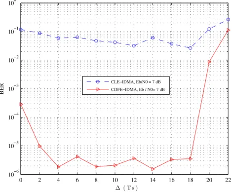
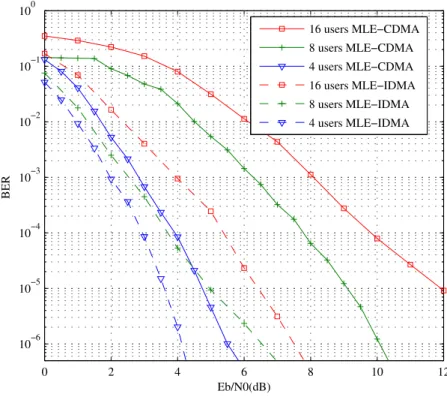
4.8 Optimal MLE-IDMA and MDFE-IDMA performances for various ∆ values, where each 1 delay of ∆ equals one symbol duration (Ts). 80 4.9 Performance of MLE-MUD receiver for different number of users in frequency selective channels. . . 81
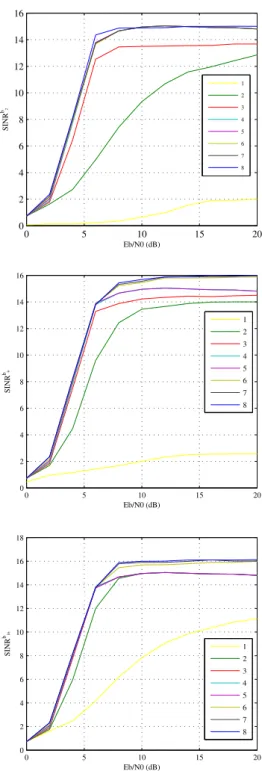
4.10 The improvement of SINR in crossover feedback filters within MLE-IDMA iterations. . . 82
4.11 Performance of MDFE-MUD receiver for different number of users in frequency selective channels. . . 84
4.12 The improvement of SINR in crossover feedback filters within cen-tralized MDFE-IDMA iterations. . . 85
4.13 Effect of lower coding rate on MDFE performance. . . 86
4.14 Performance comparison between optimal MLE-IDMA and MDFE-IDMA receivers employing 1/8 convolution coding. . . 86
4.15 Impact of FEC on MLE-IDMA systems performances. . . 87
4.16 Impact of FEC on MDFE-IDMA systems performances. . . 88
4.17 CLE-IDMA performance for perfect channel assumption and LS channel estimations. . . 89
4.18 MDFE-IDMA performance for perfect channel assumption and LS
channel estimations. . . 90
4.19 Underwater shallow water transmission scenario. . . 91
4.20 Normalized channel impulse response for user one. . . 91
4.21 Normalized channel impulse response for user two. . . 91
4.22 Impact of feedback delay ∆ on MLE-IDMA and MDFE-IDMA performances. . . 92
4.23 Impact of FEC on MLE-IDMA and MDFE-IDMA performances. . 93
5.1 The general multiuser DMDE structure. . . 96
5.2 BER vs. Eb/N0 performance of optimal DDFE-MUD system for 8 and 16 users in frequency selective channels. . . 97
5.3 The proposed iterative PIC-DDFE-IDMA receiver structure. . . . 98
5.4 BER vs. Eb/N0 performance of optimal PIC-DDFE-IDMA system for different number of users in frequency selective channels. . . . 102
5.5 MMSE curve for PIC-DDFE-IDMA for different number of users. 103 5.6 The improvement of SINR in crossover feedback filters within cen-tralized PIC-DDFE-IDMA iterations. . . 104
5.7 The iterative channel estimator structure. . . 105
5.8 BER vs. Eb/N0 optimal PIC-DDFE-IDMA performance for LS and perfect channel estimations. . . 107
5.9 Effect of coding rate on PIC-DDFE-IDMA receiver for 8 users. . 109
5.10 Performance comparison between centralized and decentralized IDMA receivers for 1/8 convolution code. . . 109
5.11 mmse vs SNR Performance comparison between centralized and decentralized IDMA receivers for 1/32 convolution code, 8 users. 110 5.12 Performance comparison different coding types for PIC-DFE-IDMA in shallow water channels. . . 110
6.1 Adaptive MDFE-IDMA performances for two users. . . 115
6.2 Adaptive MDFE-IDMA performances for four users. . . 115
6.3 Adaptive MDFE-IDMA performances for eight users. . . 116
6.4 MMSE performance of adaptive MDFE-IDMA for two users. . . . 117
6.6 MMSE performance of adaptive MDFE-IDMA for eight users. . . 118 6.7 Two-user uplink transmission scenario. . . 119 6.8 BER vs. Eb/N0 performance for DLE, DDFE, and MDFE in
mul-tipath fading channels. . . 119 6.9 Average least square error versus iteration number at Eb/N0=10
dB (1 iteration= 1 symbol period). . . 121 6.10 Scatter plot of the equalized symbols for both users using MDFE
atEb/N0=10 dB. . . 121 6.11 BER vs. Eb/N0 performance comparison of PIC-DDFE-IDMA
and MDFE-IDMA using optimal and adaptive algorithms. . . 122 6.12 Performance of PIC-DDFE-IDMA in underwater acoustic shallow
channels . . . 122 6.13 BER vs. Eb/N0 of PIC-DDFE-IDMA and MDFE-IDMA for
dif-ferent numbers of users. . . 127 6.14 Performance comparison of optimal multiuser detectors for wireless
channels. . . 128 6.15 Performance comparison of optimal multiuser detectors for
2.1 Power delay profile examples of ITU channel models. . . 16 2.2 Look up table for the convolutional encoder (2,1,4). . . 24 6.1 Complexity comparison between rake IDMA, MDFE-IDMA and
PIC-DDFE-IDMA for K=8, L=16, It=8, Itc=4, Nf=Nb=Nc=16 utilizing NLMS algorithm. . . 125 6.2 Complexity comparison between rake IDMA, MDFE-IDMA and
PIC-DFE-IDMA for K=8, L=16, It=8, Itc=4, Nf=Nb=Nc=16, No=Nf +Nb, N• = (K−1)Nc+No utilizing RLS algorithm. . . 126
Introduction
1.1
Introduciton
With higher demand of using personal communications utilities, the communi-cations technologies have experienced a significant development in recent years. To support this upswing of communication systems market, the communication systems must cope with the formidable challenges that stem from channel fading, multipath effects and multiaccess interference. The design of channel equalization and multiaccess techniques has a significant effect in developing low complexity systems that can eliminate channel disruptions, and in turn, communicate at high data rate.
Within high-speed transmission in multiaccess communication scenarios, the equalization process for multipath selective channels is an important issue, such that, it needs to be able to remove both intersymbol interference (ISI) and mul-tiple access interference (MAI), simultaneously. The multipath fading character-istic of the communication channel and the multiuser transmission are the main reason behind producing ISI and MAI, respectively. ISI is often neglected for low-rate multiuser systems [1]. However, for high-rate systems, ISI cannot be ignored. In fact, the ISI with MAI represent the main obstacle to the overall system performance [2].
sK hk hK h1 y υ s1 sk
Figure 1.1: A ultiuser transmission scenario in multipath fading channels.
1.2
Literature review
1.2.1
Development of Multiuser Communications
When digital modulated symbols are transmitted through multipath fading chan-nels, the induced ISI of the received signal is the main reason for the high Bit Error Rates (BER). However, in multiuser transmission environments, MAI has an equally significant impact as ISI, thus, both effects should be jointly eliminated at the receiver.
Within multiuser communications, multiple transmitters are enabled to send information simultaneously through multipath fading channels as shown in Fig.1.1. The multiuser communication technique had been firstly invented by Thomas A. Edison in 1873 to transmit two telegraphic messages in the same direction through the same wire [3]. Nowadays, there are many types of multiuser communication systems in which their receivers obtain the superposition of the signals sent by the active different transmitters occur unintentionally owing to non-ideal effects [4].
time division multiple access (TDMA), code division multiple access (CDMA), and interleaved division multiple access (IDMA). In FDMA, each user employs a specific frequency band for transmission. This system has been used in 1G mobile phone systems such as advanced mobile phone systems (AMPS). While in TDMA, the users are distinguished employing a specific time slot for each user to prevent interference between users [6]. TDMA is used in 2G mobile commu-nications known as global system for mobile commucommu-nications (GSM) .
On other hand, in CDMA systems, each user employs specific spreading code with good auto-correlation and cross-correlation properties that enables the re-ceiver to successfully separate the user’s data symbols; for this reason, many researchers have used this system as a multiuser detection (MUD) in multipath delay spread channels [7] [8] . This means that all users can utilize the whole bandwidth and time resources at the same time [9].
Interleave division multiple access (IDMA) is a recent multiple access tech-nique for new wireless communication systems, which unlike CDMA, it employs distinct chip-level interleavers to separate each user’s data[6]. The IDMA receiver uses a simple chip-by-chip iterative MUD strategy for jointly removing ISI and MAI. Thus the complexity of the MUD in an IDMA system is a linear func-tion of the number of users [10] and is much simpler than the MUD algorithms used in CDMA systems . Moreover, within the coded iterative turbo receiver design, IDMA showed higher performance than CDMA receiver for multipath fading channels [11].
During last few years, many works have been undertaken around IDMA topic in terms of the type of channel coding, detection algorithm and equalization tech-niques. Generally, within IDMA receiver, the symbol detection taken place by exchanging extrinsic information between Gaussian Chip Detector (GCD) and Soft Input Soft Output (SISO) decoders, while in [12], Probablistic Data Associ-ation (PDA) has been employed instead of GCD to provide lower complexity and faster convergence of the turbo receiver. On other hand, the easily integration of IDMA receiver with Orthogonal Frequency Division Multiplexing (OFDM) [13] and Multi Input Multi Output (MIMO) systems [14] to produce parallel flat fading subchannels in frequency selective channels and higher channel diversity,
respectively, have encoraged reserachers to propose more techniques and algo-rithms that can improve system performance regarding to OFDM-IDMA and MIMO-OFDM-IDMA systems [15] [16].
OFDM-IDMA combines advantes of OFDM and IDMA to jointly mitigating ISI and MAI interferences, however, it also suffers from high sensitivity to carrier frequency offsets (CFO) caused by the Doppler shift or the mismatch between the local oscillators of transmitter and receiver [17]. Especially for uplink OFDM-IDMA transmission, although the desired user’s CFO can be compensated by a signle user detector, however, the residual CFOs from other users are still intro-duce an additional interference. New schemes have been proposed to mitigate CFO and improve detection in OFDM-IDMA system [18] for multipath fading channels, however, for fast fading time selective channels, the effect of CFO in-terference on the received signal grows significantly. Therefore, applying time domain equalization for jointly removing MAI and ISI in uplink IDMA system is better solution to prevent CFO and provide higher equalization efficiency.
1.2.2
Equalization
The speed of data transmission over multipath fading channels is usually limited by channel distortion that causes ISI in single user transmission scenario or both ISI and MAI in multiuser transmission systems. Practically, the channel impulse response is unknown. However, training symbols can be utilized for estimating channel impulse response, and in turn, it could be used to remove channel effects on the received signal by implementing an inverse filter. This is the aim of using equalizers.
When more than one version of the transmitted signals arrive to the receiver with different delay times, it implies that there are several propagation paths between the transmitter and the receiver, which are referred to as multipath phenomenon. This phenomenon can be modeled by a finite impulse response (FIR) filter. The multipath channels have a significant effect on the system performance, thereby providing another good reason for channel equalization [19]. The objective of the equalizer is to calculate the taps of a filter such that the convolution of the impulse response of the equalizer filter and the channel impluse
response results in producing 1 at the center tap and have nulls at the other points within the filter span. The filter coefficients can be formulated by utilizing two main techniques: automatic synthesis and adaptation [20]. In the first method, the error signal is obtained by comparing the received training signal with the stored training signal which is used later to determine the coefficient taps of the inverse filter. However in the second method, the error signal is calculated by subtracting the output of the equalizer and the output of the decision device. Al-though, the training symbols have benefit in determining channel characteristics, however, it also present main drawback in producing transmission overhead[21].
1.2.3
Adaptive Equalization
Adaptive equalization is an effective process that mitigates the received signal dispersion caused by signal propagation in multipath channels [22]. Adaptive filters are the main part within adaptive equalization and they can offer a perfor-mance improvement over filter designs whena priori knowledge of a process and its statistics are available. Hence, they have been used in many applications such as communications, control, robotics, sonar, radar, seismology and biomedical engineering. In general, the filtering process can be characterized by filtering, smoothing, prediction and deconvolution processes [23], also according to their transfer function types they can be categorized as linear and non-linear filters.
1.2.3.1 Linear Filters
A linear adaptive filter has a linear transfer function such that the input and the output are related with a linear combination at any moment in time between adaptation operations [24]. There are three types of linear adaptive structures commonly used
- Transversal - Lattice predictor - Systolic array.
Delay Delay Delay
b(M−1)
s(n) s(n−1) s(n−2) s(n−(M−1))
b(0) b(1) b(2)
r(n)
Figure 1.2: Transversal filter structure.
Guarantee of stability and global convergence are two good properties of transver-sal linear filters which made it more popular than the other types. It is sufficient to say that for a givenMth order FIR filter, given in Fig.1.2, the output sequence r(n) can be defined as follows
r(n) = MX−1
k=0
b(k)s(n−k), (1.1) where b(k) are fixed filter coefficients, value n represents the current discrete-time instant, and (n −k) represents the previous kth instant. Whenever the filter coefficients are known, then the FIR filter can be completely defined. These coefficients can be determined using optimal solutions or employing adaptive algorithms.
There is no unique adaptive algorithm for linear filtering problems. However, based on the problem requirements, various algorithms and approaches have been proposed such as stochastic gradient approach and least square estimation (LSE) [25].
Stochastic Gradient Approach - This approach utilizes a transversal struc-ture. The optimization of transversal weights is taken place by using least mean square (LMS) algorithm. The LMS algorithm is defined by the fol-lowing equation
w(k+ 1) =w(k) + 2ηe(k)s(k), (1.2) where
s(k) = [s1, s2, . . . , sp]T, the tap vector,
ηis the learning rate parameter and the obtained errore(k) is a scalar error which is given by
e(k) =s(k)−ˆs(k) (1.3) where ˆs(k) is the estimated transmitted symbol. The LMS algorithm known to be slow to converge and dependent on the ratio of the largest to smallest eigenvalue of the correlation matrix of the tap inputs. Nevertheless, because of it’s simplicity, it is the most popular algorithm and under right conditions can perform very adequately.
Least Square Estimation (LSE) - Block estimation and recursive estimation are the two methods used for formulating LSE algorithm which minimizes the sum of square errors between the desired and the actual filter output. In the first method, the blocks of equal time length are constructed from the input data sequence and processing proceeds block by block. While the second method uses the idea of state and it could be seen as a special case of Kalman filter. The general term of Kalman filtering can be defined as follows [25]
x(k+ 1) =x(k) +K(k)i(k), (1.4) whereK(k) is the Kalman gain matrix at instance k, i(k) is the innovation vector at instance k, and x(k) is the state of instance k. The vector i(k) consists of the new information that is presented to the filter for instance k.
1.2.3.2 Non-Linear Adaptive Filter
Non-linearity refers to the lack of linear combination between input and output at any moment in time [26][27]. The applications of signal processing are often assuming system linearity, however, in practice, the system performance is lim-ited by the non-linearity characteristic. Thus, more concern has been given to design non-linear filters. Volterra filter [28] is an example of nonlinear adaptive filter which can be seen as a type of polynomial extension to the linear adaptive
filter. Volterra filter can keep its output linear with respect to high power impulse responses or system coefficients. Although utilizing nonlinear filters will improve the learning efficiency, however, this comes at the expense of more complex math-ematical analysis of the problem.
1.2.4
Multi-Dimensional Equalization
Within multiuser equalization, in addition to using the previously detected sym-bols of the user of interest, estimates of the current symsym-bols of the remaining active users are also required to jointly remove both MAI and ISI effects [29] for the current symbol detection. Blind equalization, which only needs a received signal and desired output signature, has been used with DFE in such situations [7].
Multidimensional equalizers are typically proposed to reduce the adjacent channel interference that can often appear in mobile data transmission [30]. This method has been exploited with two user transmission for co-channel interference suppression [8]. In these receivers, referred to as centralized equalizers, the MAI has been subtracted by using crossover filters in conjunction with CDMA or IDMA. On the other hand, decentralized equalizers are obtained by removing the crossover filters.
An IDMA detector with DFE multidimensional equalization has been pro-posed in [31] for downlink scenarios in underwater acoustic channels. In this sys-tem, the summation of the users’ data headed by a common sequence of training symbols constructs the transmitted signal frames to be sent through the channel. Since the signal frame arriving at a specific user experiences the same channel characteristics, a single DFE equalizer is sufficient to remove the ISI from the received signal, while the MAI can be cancelled by IDMA detection. However, this approach cannot be applied to uplink scenarios, where the transmission of each user arrives at the base-station via distinct multipath channels.
1.3
Research Contributions
This work mainly concentrates on the solution to the equalization problems in multiuser systems for uplink scenario. First we proposed a centralized multi-dimentional equalizer for two user IDMA uplink system in shallow water acoustic channels [32]. Within centralized equalization, ISI is eliminated by using feed-forward and feed-backward filters, while, MAI is removed using crossover filters. A new mathematical derivation has been derived for calculating the optimal fil-ter coefficients. Then, the optimal equalizer is applied to the wireless channel environment for more than two users.
Although the proposed multi-dimensional equalizer provides higher system performance than usual rake IDMA and traditional CDMA receivers, however, it suffers from delay in converging filter taps which results in decreasing system performance, especially, at low SNR values. For this reason, A new decentralized multi-dimensional equalizer has been designed for uplink multiuser systems by replacing cross-over filters with parallel interference canceller (PIC) technique. A comprehensive study on the receiver design, performance analysis, optimization solutions and complexity comparison are also presented for both the proposed receivers. More specifically, the contributions can been listed as follows:
- The centralized multidimensional equalizer structure outlined in Chapter 4. The equalizer was employed with CDMA for two-users in shallow water acqoustic channels and adaptive algorithm has been used for determining filter taps. This thesis designed an iterative centralized multidimensional equalizer that uses IDMA. The two-user uplink scenario for shallow water acoustic channels is considered in [33]. At the receiver, for each user, a DFE equalizer has been used before IDMA detection. The IDMA detector iteratively returned the hard limited symbol to the equalizers to optimize the cost function employed in the adaptive algorithm.
- New derivations for calculating optimal filter taps are also presented in the Chapter 4. The derivations are given for both linear and DFE
equaliz-ers. Moreover, that optimal solution could be applied to both IDMA and CDMA.
- Due to delay in converging filter taps, especially cross-over filters, the cen-tralized equalization provides low performance at low SNR values. Hence, a new decentralized multidimensional equalizer is proposed in Chapter 5. A new IDMA receiver has been applied to wireless multipath fading channels in [34] and shallow water acoustic channels in [35]. The proposed receiver is a mixture between Rake IDMA and decentralized multidimensional equal-izer such that it utilizes a PIC to eliminate MAI impairments, while it applies DFE equalization to overcome ISI effects for each user. The de-sign of such a receiver obtain high system performance and lower system complexity compared to the centralized and Rake receivers.
1.4
Thesis Organization
The remaining of the thesis is organized as follows.
Chapter 2 provides preliminaries on channel models, channel encoding and fundamentals of equalization techniques. Firstly, the models of both wireless fad-ing and shallow water acoustic channels have been reviewed. Several characteris-tics of the channels are elaborated. Two types of channel encoding are presented which are convolution and trubo coding. Also the fundamentals of linear and DFE equalization techniques have been described. Moreover, joint equalization and decoding in an iterative system are illustrated for achieving higher system performance in multipath fading channels.
Chapter 3 is devoted to multiuser detection schemes, i.e CDMA and IDMA. The basic structure of both CDMA and IDMA are outlined. The iterative scheme of CDMA detection has been illustrated. The fundamental equations of IDMA for both additive white Gaussian noise (AWGN) and multipath selective channels are also provided.
Chapter 4 develops centralized multidimensional equalizer method to be ap-plied to iterative CDMA and IDMA receivers. The optimization problem for centralized multidimensional equalizers employing linear and DFE principles is
also solved, such that the determined filter coefficients give optimal performance. Comprehensive comparisons between CDMA and IDMA are carried out utilizing the proposed centralized multidimensional equalizer.
Due to delay in converging filter taps in centralized multidimensional equalizer schemes, the IDMA detector suffers in performance due to the remaining MAI effects in crossover filter taps. Thus, Chapter 5 provides a new decentralized multidimensional equalizer for IDMA detection which totaly depends on PIC op-eration to remove MAI dispersion. The structure of the proposed IDMA receiver is presented and its system performance is compared to the centralized IDMA detector for both wireless and shallow water acoustic channels.
Chapter 6 focuses on applying adaptive algorithms on the two proposed mul-tidimensional equalizers for IDMA detector. The adaptive receivers are also com-pared with rake IDMA receiver in terms of complexity.
Finally, conclusions are presented in Chapter 7 and the thesis ends with a possible line of future work.
Preliminaries: Channel Models,
Channel Encoding and
Equalization Techniques
This chapter provides a general introduction to channel models, channel encoding, MMSE equalization (LE and DFE) , and turbo equalization techniques. Channel models for both wireless and underwater shallow channels are presented, as the system performance of the proposed systems in later chapters in this thesis are evaluated for both channels. The principles of convolution and turbo coding are then explained. Furthermore, the fundamentals of MMSE equalization are presented for both LE and DFE. Finally, the turbo equalization technique is reviewed and the formulas for finding optimal filter taps are derived for both linear and non-linear MMSE turbo equalizers.
2.1
Communication Channels
The purpose of any communication system is to transmit the information signals from one point to another. The medium over which the information signals are transmitted is called communication channel which can be wire line, optical cable, wireless radio channel or acoustic channel. When data information are transmitted through the channel, it is subject to an assortment of changes. These
Receiver
LOS
Transmitter Transmitter
Receiver
Figure 2.1: The forms of wireless channel environments: LOS and NLOS
changes could be deterministic, i.e attenuation, linear and non-linear distortion, or probabilistic, i.e additive noise, multipath fading, etc.
2.1.1
Multipath Fading Channel model
Line-of-sight (LOS) and non line-of-sight (NLOS) are two general forms of wire-less channels. The absence of the direct line between the transmitter and the receiver in NLOS is the only characteristic that makes it differ from LOS. The pobability density function (PDF) follows Rician and Rayleigh distribution in LOS and NLOS, respectively [36]. Fig. 2.1 depicts these two different environ-ments. In LOS channels, the antennas receive the signal via direct path and also via different propagation paths which are created due to reflections, diffraction and scattering from natural and manmade objects. However, in an urban envi-ronment, the absence of a direct line propagation due to surrounding obstacles results in arriving signals only from the multipath propagation paths. These mul-tipath components, have a randomly distributed amplitudes, phases and angles of arrival signal such that their combination at the receiver results in a signal that can vary widely in both amplitude and phase. This phenomenon is called fading.
The signal reflections, changing of Doppler shifts and delays of multipath propagation are generally the three main effects of the fading multipath channels on the transmitted signal . During arrival of a number of the attached symbols
−1 Amplitude Time 1 0 0 1 0 1 Ts
Figure 2.2: Transmitted sequence.
0 0 0 1 −1 Amplitude Time 1 1 ISI Ts
Figure 2.3: Received sequence.
at the same time to the receiver via various multipath propagation, the receiver simply adding them together at every time instants, which inturn, results in producing inter symbol interference (ISI). Fig. 2.3 illustrates the effect of ISI on the transmitted data sequence 10010 shown in Fig. 2.2 over a fading multipath channel.
A tapped delay line (TDL) can be employed to model the multipath channels as given in Fig. 2.4 and its characteristics are often specified by a power delay profile (PDP). The pedestrian and vehicular PDP by ITU are given in Table 2.1, in which each path is distinguished by its relative delay and average power. The relative delay is an excess delay with respect to the reference time while the average power for each path is normalized by that of the first path [37].
Several small scale multipath channel parameters such as mean excess delay, root mean square (RMS) delay spread and excess delay spread which define the channel time dispersive properties can be obtained from the PDP. Mean Excess
Delay (τ) is the first moment of PDP and is defined as [38]
τ = P la2lτl P la2l = P lτlP(τl) P lP(τl) , (2.1)
where τl denotes the channel delay of the lth path while al and P(τl) denote the amplitude and power, respectively.
s(t−τL−1−...−τ2−τ1−τ0) s(t) h(t, τ0) h(t, τ1) h(t, τ2) r(t) v(t) τL−1 τ0 τ1 τ2 h(t, τL−1) s(t−τ1−τ0) s(t−τ2−τ1−τ0) s(t−τ0)
Figure 2.4: Tapped delay line channel model.
Table 2.1: Power delay profile examples of ITU channel models.
Tap Pedestrian Vehicular
Relative Delay (ns) Average Power (db) Relative Delay (ns) Average Power (db)
1 0 0 0 0
2 110 -9.7 310 -1
3 190 -19.2 710 -9
4 410 -22.8 1090 -10
5 - - 1730 -15
While, the root of second central moment of PDP is called RMS delay (στ) and its defined as
στ = q τ2−(τ)2, (2.2) where τ2 = P la2lτl2 P la2l = P lτl2P(τl) P lP(τl) . (2.3)
The characterization of the channel in time domain is defined by employing delay spread parameters. However, in frequency domain the channel is charac-terized by the coherence bandwidth (Bc) which is the range of frequencies over which the signal strength remains more or less unchanged. In general, the relation between Bc and RMS delay is an inverse proportion, that is [38]
Bc≈ 1 στ
. (2.4)
coherence bandwidth, then
Bc ≈ 1 50σl
, (2.5)
while if a correlation of 0.5 or above is taken, then the coherence bandwidth is given as
Bc≈ 1 5σl
. (2.6)
The characteristics of the transmitted signal and the properties of the channel are the two main factors for identifying the type of channel fading. The channel is called frequency selective fading channel when the bandwidth of the transmitted signal is greater than bandwidth over which the frequency response of a mobile channel has a constant gain and linear phase, i.e Bc < Bs or Ts < στ where Ts and Bs are the symbol period and bandwidth of the transmitted signal. Thus, frequency selective fading is a result of the time dispersion of the transmitted symbol within the channel.
On the other hand, the movement of the transmitter or reciever results in changing the channel response within a symbol period transmission, thus the signals transmit through a time-selective fading channel. The rapid variation of impulse response leads to a spread in the frequency domain which is known as a Doppler shift. If maximum Doppler shift denotes as (fm), then the Doppler bandwidth is given as Bd = 2fm. In general, the coherence time is related to Doppler spread as
Tc≈ 1 fm
. (2.7)
The channel behaves as fast fading under the following conditions: Ts > Tc and Bs< Bd,
while, it behaves as slow fading when
TsTc and BsBd.
2.1.2
Shallow-Water Acoustic channel Model
The underwater acoustic channel is another example of multipath medium where the signal transmits through reflections from the surface and the bottom of the
sea. In addition, it can be a time-varying channel due to the motion of the transmitter or the receiver during transmission or due to medium variability. The wave propagation in an underwater channel is mainly affected by channel variations, multipath propagation and Doppler shift with an adverse impact on achieving high data rates and transmission robustness. Furthermore, the usable bandwidth of an underwater channel is typically a few kHz at large distances. In order to achieve high data rates it is natural to employ bandwidth efficient modulation.
Most researches on underwater acoustic channels are focused on mathemati-cal models which are mainly characterized as shallow water multipath and deep vertical channels [39]. Shallow water channels are presented into two models: random time-varying filter and random statistical channel model [40], based on ray theory [41][42]. Most practical applications are preferred ray theory model over random statistical channel model due to the independency of ray trajectories on the interested used frequency [43][44].
In a shallow water channel, the acoustic waves travel through a LOS path also by bouncing from the surface and bottom [45]. The propagation of acoustic signals can be roughly estimated over a shallow water by simplifying the envi-ronment parameters. If the surface and bottom of the water are assumed to be smooth, then the expected propagation paths for the acoustic waves can be geo-metrically calculated. In general, the parameters which are mainly affecting the underwater communications are
2.1.2.1 Attenuation
The spreading and absorption are the main losses that attenuate the transmitted signal in shallow water channels. According to inverse square law, the attenuation is proportional to 1
L2, where L is the distance between the transmitter and the
receiver, for LOS propagation. As L increases, propagation occurs via reflection at the sea surface and floor boundaries where the attenuation is proportional to
1
L, and this is called cylindrical spreading. The total transmission losses (TL) for cylindrical spreading can be expressed as [46]
where a(f) is the attenuation coefficient in dB/km and can be computed as [47] a(f) =Af2+ Bfo 1 +fo f 2 + Cf1 1 + (f1/f)2 , (2.9) where A= 2.1×10⁻¹⁰(T −38)2, B = 2S×10−5 and C = 1.2×10⁻⁴
are fresh water attenuation, magnesium sulphate relaxation and boric acid relax-ation, respectively,S is the salinity in parts per thousand andf is the operating frequency in KHz. Additionally
fo= 50(T + 1), f1 = 10
T−4 100 ,
where T is the temperature in Celsius. In practice, absorption losses can be determined by [48]
a(f)<10dB. (2.10)
On the other hand, another factor in shallow water channels that has a great impact on the system performance is ambient noise. The ambient noise exists in specific places in the background of the sea such as snapping shrimp in warm waters, and also it comes from rain, breaking waves and distant shipping. The spectral density of ambient noise decreases significantly over a range of operat-ing frequencies, hence, it is not white. The comprehensive analysis of different underwater channels can be found in [49].
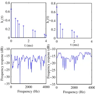
Figure 2.5: Impulse response of shallow water channel.
2.1.2.2 Multipath Propagation
The phenomenon of multipath within an underwater acoustic channel is mainly produced by the geometry of the water environments. The water environments include different reflectors and scatters, bottom boundaries, surface reflectors, and heterogeneity of sea water. The multipath underwater channels are usually time-varying channels, thus it is impulse responses can be characterized as doubly spread. Doubly spread referred to delay and Doppler spread. Frequency selective fading and time dispersion are the two main effects of the delay spread, while Doppler spread results in creating frequency dispersion and time-selective fading effects. The multipath delay profile of a shallow water channel depicted in Fig.2.5 is experimentally obtained by sea-trials conducted by Newcastle University in the North Sea.
2.1.2.3 Doppler shift
Doppler shift is produced by the movement of the transmitter or receiver and varying reflections at the surface and bottom of the sea. The reflection and scattering of sound waves on the surface of the sea is based on the Rayleigh parameter [47]. Rayleigh parameter can be calculated as
R = 2πρsinφ
λ , (2.11)
whereλis the wavelength of the sound wave,ρ is the rms roughness wave height, and φ is the grazing angle. For R <<1 indicates the surface is perfectly smooth and behaving principally as reflector. In contrast, for rough surface, the Rayleigh coefficientR >>1, and the surface acts as a scatterer. The reflection loss can be computed as
µR = 20log10R. (2.12)
In general, there is a vast difference in complexity between the signal reflec-tions on the surface of the sea and the seabed. The high changing of the acoustic properties in the bottom and the gradual changing of the sound velocity and density due to layered bottom makes seabed more complex than the sea surface.
2.2
Channel Encoding
Within communication systems, the prime requirement of transmitting informa-tion over multipath channels is reliability. Hence, the channel encoding techniques have occupied a high interesting by the researchers in modern communication systems. The detection capability and error correction are the main two charac-teristics for good coding schemes. In this section, we will give a brief introduction into the field of channel coding. To this end, we will describe two common chan-nel encoders which are widely used in communication systems. These encoders are based on convolution coding and turbo coding which are mainly employed in our proposed receivers in the following chapters.
u0 (1,1,1) (0,1,1) (1,0,1) x2 x1 x3 u1 u1 u−1
Figure 2.6: (3,1,3) convolutional encoder.
2.2.1
Convolution Coding
2.2.1.1 EncoderThe convolutional codes generally are specified by N = number of output bits,
K = number of input bits, M = number of memory registers.
The efficiency of the code can be measured by the code rate (K/N). Fig. 2.6 depicts a (3,1,3) convolutional encoder with rate 1/3. The module-2 adders are the generators for the three outputs, and their inputs are selected by a specific generator polynomial (g) for each output bits, that is
x1=mod2(u1+u0+u−1),
x2=mod2(u0+u−1),
x3=mod2(u1+u−1).
The polynomials can create codes having completely different properties. For any M order code, there are many choices for polynomial which will not all result in output codes with good error protection properties. The complete list of these polynomials can be found in [50].
States are referred to the number of combination bits in the shaded registers and are defined by
u1 u1 u0 u−1 (0,1,1) x2 x1 x3 (1,0,1)
Figure 2.7: The systematic (3,1,3) convolutional encoder. x1 u1 u1 u0 u−1 (1,1,1,1) x2 u−2 (1,1,0,1)
Figure 2.8: (2,1,4) convolutional en-coder.
Number of states = 2L,
where L represents the constraint length of the code and it is equal toK(M−1). The shaded registers in Fig. 2.6 have a constraint length of 2. The convolutional code could be systematic or non-systematic. In systematic convolution coding, the known sequence of the input bits are forwarded with the output bits. The systematic version of Fig. 2.6 is shown in Fig. 2.7. Even though both types of convolution codes have the same protection properties, however, systematic codes are preferred over non-systematic due to less hardware requirement for encoding, quick looking permission and the absence of catastrophically error propagation. Thus, systematic convolution codes are used in Trellis Coded Modulation (TCM) and turbo codes.
Table lookup mechanism is usually employed for encoding purpose which con-sists of the input bits, the output bits and the state of the encoder. Table 2.2 gives the look up table for (2,1,4) convoultional code shown in Fig. 2.8.
State, tree and trellis diagrams are three ways to look at the encoder and understand the operation of encoding. Trellis diagram is the most preferred over the others because it represents linear time sequencing of events. Within the trellis diagram, the x-axis is discrete time and all possible states are shown on the y-axis. Each horizontal transition indicates arrived bits, and each transmitted code word has its own trellis diagram. The trellis diagram always starts at state
Table 2.2: Look up table for the convolutional encoder (2,1,4).
Input Bit Input State Output Bits Output State
0 0 0 0 0 0 0 0 0 1 0 0 0 1 1 1 0 0 0 0 0 1 1 1 0 0 0 1 0 0 1 0 0 1 0 0 0 0 1 0 1 0 0 0 1 1 0 1 0 0 1 1 0 1 0 0 1 1 0 1 0 0 1 1 0 1 1 1 0 1 0 1 0 1 0 0 1 1 0 1 0 1 1 0 0 0 0 1 1 0 0 1 0 1 0 0 0 1 0 1 1 0 1 1 1 1 1 0 0 1 1 0 0 1 0 1 1 1 1 1 0 1 0 1 1 1 0 1 1 1 1 0 0 1 1 1 1 1 1 0 1 1 1 1
000 and it becomes fully populated after L bits. The transitions then repeat from this point as it is shown in Fig. 2.9. The encoding process of the incoming bits is easy using trellis diagram, basically branching up for a 0 and down for a 1 bit. An example of encoding the sequence (10100) is depicted in Fig. 2.10. The path taken by the bits of the sequence determines the output code sequence.
2.2.1.2 Decoder
The main objective of the decoder operation is to provide the highest possibility of estimation for the uncoded transmitted bits from the received coded bits. The decoder type depends on the type of the demodulator output such that the decoder is referred to ashard-decision decoding when the demodulator carries out a binary decision concerning the received bit (i.e hard-decision demodulation). While, the decoder is referred to assoft-decision decoding when the demodulator
repeats 010 011 100 101 110 111 000 001 0(00) 0(00) 0(00) 0(00) 0(00) 1(11) 1(11) 1(11) 1(11) 1(11) 1(00) 1(00) 1(00) 1(00) 0(11) 0(11) 0(11) 0(11) 0(10) 0(10) 0(10) 1(10) 1(10) 1(10) 0(01) 1(01) 0(01) 1(01) 0(01) 1(01) 0(11) 1(00) 0(01) 1(10) 1(11) 0(00) 1(01) 0(10) repeats
Figure 2.9: Trellis diagram of (2,1,4) code.
outputs includes multilevel confidence measures concerning the probability of a binary one and zero (i.e soft-decision demodulation) .
In general, the soft decoder is used in iterative detection due to it’s higher efficiency than hard decoder. Soft decoding relies on symbol probability decoding algorithms for the iterative processes. The well-known and widely used algorithm for soft decoding is called a posteriori probability (APP). The APP algorithm is also known as BCJR or the forward-backward algorithm. The APP algorithm was originally invented by [51] to provide the maximum probability of correction for each symbol, and this referred to as the maximum a posteriori probability (MAP) algorithm. With the invention of turbo codes, the APP became the prime representative of the so called soft-in soft-out (SISO) algorithms which is used for obtaining probability information on the symbols of a trellis code.
010 011 100 101 110 111 000 001 1(11) 0(11) 1(01) 0(00) 0(10) u4, x4 s1 s2 s3 s4 s5 s0 u0, x0 u1, x1 u2, x2 u3, x3
Figure 2.10: Encoding process for input sequence.
Demodulation Convolutional Encoder Modulation SISO Decoder x y N(0, σ2) u Figure 2.11: Notation.
2.2.2
Soft Input Soft Output Decoding (SISO)
In order to simplify SISO decoding description, we establish a notational con-vention as in Fig. 2.11. The trellis code shown in Fig. 2.10 consists of five sections. The transmitted code signal is x = [x0, ..., x4], and the data symbols
are u= [u0, ..., u4]. The purpose of SISO decoder is to compute thea posteriori
demodu-lator. In general, the SISO decoders have three inputs and generate two outputs. Regarding the notation shown in Fig. 2.12, the systematic part, parity part of the received codeword anda priori probabilities on information symbols are the three inputs of the SISO decoder. The outputs of a SISO decoder are APP(ut) which is an estimate of ut given all observations and given all a priori proba-bilities, and Ext(ut), is a type of APP(ut) independent of rtp and Π(ut), where Π denotes the interleaving operation. The a priori probability input is used for iterative decoding, whereas for non-iterative decoding its values are zeros.
MAP algorithm
Conceptually, the MAP algorithm calculates the probability that the encoder crossed a specific transition in the trellis, i.e. Pr[st = i, st+1 = j|y], where st is the state at time t, and i and j are the previous and present states, respectively [52]. This probability can be computed as the product of three terms
Pr[st=i, st+1=j|y] =
1
Pr(y)αt−1(i)γt(i, j)βt(j). (2.13) The internal variables of the algorithm are given by the values of α and can be determined by the forward recursion
αt−1(i) =
X
statesl
αt−2(l)γt−1(i, l). (2.14)
Employing previously calculated α values at time t−2 and the sum over all statesl at timet−2 that connect with state iat timet−1, the estimation of the α values are obtained during forward recursion at time t−1. The initial values for α are
α(0) = 1, α(1) = α(2) =α(3) = 0.
On other the hand, the values ofβare calculated by using backward recursion βt(j) = X
statesl
βt+1(l)γt+1(l, j), (2.15)
and initialized as β(0) = 1, β(1) = β(2) = β(3) = 0 which enforces the termi-nating condition of the trellis code. The overall states l summation takes place
SISO
Extrinsic output APP terms Systematic part Parity part A priori probabilitesFigure 2.12: SISO decoder.
at time t+ 1 to which state j at time t connects. The values of γ are the con-ditional probabilities which are the inputs to the algorithm, while, γ(j, i) is the joint probability that the state at time t+ 1 is st+1 =j and that yt is received. This can be calculated as
γt(j, i) = Pr(st+1 =j, yt|sr=i) = Pr[st+1 =j|st=i]Pr(yt|xt). (2.16) where the first term Pr[st+1 = j|st = i]Pr is the a priori transition probability which is related to the probability of ut. Hence, this transition probability can be abbreviated as
pij = Pr[st+1 =j|st=i] = Pr[ut]. (2.17) While the second term in (2.16) is the conditional channel transition probability, given that symbol xt is transmitted. Hence, (2.16) can be rewritten as follows
γt(j, i) = Pr[ut]Pr(yt|xt). (2.18) The output of the iterative decoder can be derived to calculate a priori prob-ability Pr(ut), while, the joint probability can be computed as
Pr(yt/xt) = n Y l=1 Pr(ytl/xtl) = n Y l=1 1 √ 2πσ2e −1 2σ2(ytl−xtl)2 (2.19)
where xtl and ytl are single transmitter and receiver bits within codewords, re-spectively;n is the number of bits in each codeword; andσ2 is the noise variance,
j i
Figure 2.13: Transitions corresponding tout.
summation over all transitions of the a posteriori transition probabilities (2.13) can be used to compute the a posteriori symbol probabilities Pr[ut|y] regarding tout = 1 andut= 0, separately, that is
p[ut= 1|y] = 1 Pr(y) X solid αt−1(i)γt(i, j)βt(j), (2.20) p[ut= 0|y] = 1 Pr(y) X dashed αt−1(i)γt(i, j)βt(j), (2.21)
where solid transition correspond tout = 1, and the dashed transitions correspond tout = 0 as illustrated in Fig. 2.13. Hence, the outputa posteriori LLR can be determined as L(ut|y) = log p[ut= 1|y] p[ut= 0|y] = log " P (i,j)∈A(u)αt−1(i)γt(i, j)βt(j) P (i,j)∈B(u)αt−1(i)γt(i, j)βt(j) # , (2.22)
where A(u) and B(u) denote the solid and dash transition states, respectively. The mathmatical operations of the real numbers involved in the MAP algo-rithm results in a high complexity in the hardware implementations [51]. Trans-ferring the algorithm to the logarithm domain leads to reduce the algorithm
complexity which is called Max-log-MAP algorithm [53][54]. This technique uti-lizes an approximation which drastically reduces the complexity however, at a cost of performance degradation. The lower performance problem of Max-log-MAP algorithm can be solved by using Log-MAP algorithm [55] that corrected the approximation used in the Max-Log-MAP algorithm.
2.2.3
Turbo Coding
2.2.3.1 Turbo EncoderAccording to Shannon, when a message is sent infinite times, each time shuffled randomly, then the ultimate code can be obtained. This means that the receiver has infinite copies of the message, which can be used by the decoder to decode the message sent with near error-free probability. Turbo code, aims to achieve this performance, albeit with messages being sent only two or three times.
Fig. 2.14 shows the turbo encoder which consists of two recursive systematic convolutional (RSC) encoders. The output of the two encoders are approximately statistically independent of each other due to using the interleaver between them. Although, its possible to utilize more than two components in turbo codes, how-ever, we concentrate on the standard turbo encoder structure which is using two RSC codes. Each half rate RSC encoder generated a systematic output which includes the original and parity information. Half of the parity output bits from the encoders are punctured so as to produce one half of the overall coding rate. Hence, after puncturing, the output of the turbo encoder is a multiplexing of the systematic bits with the punctured parity bits.
2.2.3.2 Turbo Decoder
The turbo decoder employs maximum likelihood detection (MLD), where the re-ceived signal after modulation is fed to the decoders which work on the signal amplitude to output soft decision bits. The MLD is known as maximum MAP when it is used by turbo decoding [56]. Within turbo decoding, the MAP algo-rithm works iteratively to improve the system performance, where the number of iterations depends on the SNR value. The higher the SNR, the less iterations are required.
{dp1} Π RSC1 RSC2 Multiplexing {d} {c} {dp2} Puncturing and
Figure 2.14: Turbo encoder.
The SISO decoder is the most important component in turbo decoder, because it computes a posteriori probabilities on bits. Corresponding to the two RSC encoders at the transmitter, the turbo decoder includes two SISO decoders that are connected by interleaver as shown in Fig. 2.15. The number of SISO decoders is equal to the number of RSC encoder components. During processing of the received signal, each SISO decoder computes the information about the data bits and extrinsic information about the coded bits, which in turn is sent to the other SISO decoder. The key idea of exchanging soft extrinsic bits between these two SISO decoders can greatly improve the system performance.
The channel output values are taken by the first SISO decoder which produces the soft output as its estimate of the data bits during the first iteration. Then the soft output bits are interleaved and taken as a priori information for the second SISO decoder. The second decoder employs this a priori data and the received data bits to obtain the estimate of the data bits. Similarly, the estimated output bits of the second decoder are deinterleaved, which are treated as apriori
information by the first SISO decoder during second iteration. The exchanging of
apriori information between the SISO decoders in each iteration leads to improve
Figure 2.15: Turbo decoder.
2.3
Equalization Principles
The amplitude and phase dispersion of the channels leads to a very high BER at the receiver due to the effects of ISI. In order to solve the problem of ISI caused by the multipath channels, in spite of utilizing channel encoders, equalizers are also required. The receiver design depends on the fact that the channel transfer function is known. However, in practical communications applications, the channel transfer function is not known to the receiver to eliminate channel effects.
The optimum equalizer can be obtained by using maximum likelihood se-quence detection (MSLE) which depends on the criterion of minimum proba-bility of error. However, MSLE has high complexity. Alternatively, employing linear combinations of the received signal symbols to remove ISI is a suboptimal method of equalization and it is called Linear Equalizer (LE). LE has a good performance in slow fading channels, however, it has limited performance in fast fading channels. Therefore, the decision feedback equalizer (DFE) has been de-signed to mitigate fast fading through using feedback filter to remove the effect of the ISI caused by previous transmitted symbols.
Having a transmitter as shown in Fig. 2.16, {c}NdRc−1
Figure 2.16: Transmitter.
Figure 2.17: Linear equalizer structure.
data after error control encoding withRc and Nd representing the code rate and number of transmitted data bits, respectively. After encoding, the codeword bits are mapped to symbols {sk}Nn=0s−1, where Ns is the number of the transmitted symbols, which are taken from a M-ary symbol alphabet: χ,{α1, ..., αM} with E{χ}= 0 andE{|αq|2}= 1.
We assume L paths channel model, with complex-valued fading coefficients
{h(l)}Ll=0−1. The received signal can then be represented as y(n) =X
l
h(l)s(n−l) +υ(n), (2.23) whereυ(n) are complex-valued samples of zero-mean AWGN with varianceσ2
v = N0/2.
2.3.1
Linear Equalizer
The simplest suboptimum solution to remove ISI in the received signal is through the use of LE as shown in Fig. 2.17. This method generally incorporates a transversal filter (f), and the complexity of the filter linearly depends on the channel’s transfer function.
Within communication systems, the transmitted data symbols s(n) are re-ceived in the presence of multipath channel effects and additive noise υ(n). The signals s(n) and υ(n) are assumed uncorrelated. Due to channel memory, each received symboly(n) contains contributions form boths(n) and prior transmitted symbols. Hence, the received data symbols in (2.23) can be rewritten as follows:
y(n) =h(0)s(n) + L X l=1 h(l)s(n−l) | {z } ISI +υ(n), (2.24)
where the second term on the right hand side describes the ISI caused by the prior transmitted symbols.
Assuming that the detected symbols ˇs(n) after the decision device are free of errors, i.e the ˇs(n −∆) can be replaced with s(n −∆), then the criterion for determining transversal filter coefficients (f) is obtained by minimizing the variance of the error signal, which can be given as
e(n−∆) =s(n−∆)−sˆ(n−∆). (2.25) where s(n−∆) = ˇs(n−∆) by assuming the correct detection of the equalized symbol. The received observed symbols can be expressed in column form as
y= y(n) y(n−1) y(n−2) . . . . y(n−Nf + 1) , (2.26)
where Nf is the length of transversal filter taps. Moreover, the processs(n−∆) is jointly wide-sense stationary with y, hence the covariance quantities
Ry =E yyH =HRsHH +Rv, (2.27) rsy=E s(n−∆)yH =λsHH, (2.28) are independent of n, where
λs= [0 0| {z. . . }
∆
σs . . . 0 0],
is a vector of lengthNf which all its element are zeros except element with position ∆, σs =E[s(n−∆)s(n)∗], (.)H denotes the conjugate transpose operation, H ∈
CNf×(L+Nf−1) is the channel matrix constructed from the estimated channel taps
during training mode, i.e.
H= h(0) . . . h(L−1) 0 . . . 0 .. . . .. . .. . .. ... ... 0 . . . 0 h(0) . . . h(L−1) , (2.29)
and Rs ∈C(Nf+L−1)×(Nf+L−1) is the covariance matrix.
The covariance matrix
R, σs rsy rH sy Ry , (2.30)
is assumed to be positive-definite and invertible. The positive-definiteness of R
guarantees that both Ry and the Schur complement of R are positive-definite
matrices too, i.e.
Ry>0, Rδ ,σ−rsyR−y1rHsy >0,
where the Schur complement is denoted by Rδ [25]. The optimal filter taps can be determined by solving
∆J = min
f E|ek(n−∆)|
2. (2.31)
Moreover, (2.25) can be rewritten as
e(n−∆) =s(n−∆)−sˆ(n−∆) =s(n−∆)− lf=XNf−1 lf=0 f(lf)y(n−lf). (2.32)
By collecting the coefficients of f(lf) in row form
fH ,[f(0) f(1) · · · f(Nf −1)], (2.33) the expression in (2.32) can be rewritten in vector form as follows
e(n) = s(n−∆)−fHy. (2.34) By substituting (2.34) in (2.31), the optimization problem can be written as follows
∆J = min
f E|s(n−∆)−f
H
y|2. (2.35)
The right hand-hand side of (2.35) can be expanded as follows ∆J = min f E h sk(n−∆)−fHy s(n−∆)−fHyHi = min f E s(n−∆)−fHy s(n−∆)H −yHf = min f E[s(n−∆)s(n−∆) H −s(n−∆)yHf −fHys(n−∆)H +fHyyHf]. (2.36)
In turn, with the aforementioned definitions, (2.36) can be rewritten as follows ∆J = min f (1−rsyf−f HrH sy+fHRyf) . (2.37)
The optimal fH is determined by differentiating ∆J with respect to f and setting it to be equal to zero.
∂∆J ∂f =−rsy+f HR y, (2.38) hence, fH =rsyR−y1. (2.39)
By substituting (2.39) into (2.37), we can find the minimum mean square error of linear equalizer (MMSELE), that’s
MMSELE = 1−rsyR−y1r
H
sy. (2.40)
2.3.2
DFE Equalizer
Within the DFE structure, in addition to the transversal filter in the feed forward path, a feedback filter is also employed in order to feedback previous decisions and utilize them to reduce ISI as shown in Fig. 2.18. The utilization of the decision device in DFE equalization provides it with nonlinear characteristic. The decision device tries to determine which symbol of a set of modulation levels was actually transmitted. After each symbol estimation, the DFE equalizer with the aid of filter structure can compute the channel effect on following symbols and compensate the input of the decision device for the next samples. This postcursor channel removal takes place by using a feedback filter structure.
By defining the returned symbols through the feedback filter as
s= s(n−∆) s(n−∆−1) . . . . s(n−∆−Nb) , (2.41)
Figure 2.18: DFE equalizer structure.
and using the same definitions for the observed symbols, estimated symbols and filter taps given in LE section, the covariance matrix
R, Rs Rsy RHsy Ry , (2.42)
is assumed to be positive-definite and invertible, where Rsy ∈ CNb×Nf. The
positive-definiteness ofRguarantees that both Ry and the Schur complement of R are positive-definite matrices too, i.e.
Ry>0, Rδ ,Rs−RsyR−y1R
H
sy>0,
where the Schur complement is denoted by Rδ [25].
For the DFE structure, the error signal given in (2.25) can be rewritten as follows e(n−∆) =s(n−∆)− NXf−1 lf=0 f(lf)y(n−lf) + Nb X lb=1 b(lb)s(n−lb). (2.43)
Moreover, the error signal can be written in vector form as
e(n) = bHs−fHy, (2.44) where
hence, the optimization problem in (2.31) becomes ∆J = min f,b E |bHs−fHy|2, (2.46) ∆J = min f,b E (bHs−fHy)(bHs−fHky)H = min f,b (b H E[ssH]b−bHE[syH]f−fHE[ysH]b+fHkE[yyH]fk). (2.47) By substituting Rsy, (2.47) can be rewritten as
∆J = min f,b (b H Rsb−bHRsyf−fHRHsyb+f H Ryf). (2.48)
The optimal fH is determined by differentiating ∆J with respect tof, thats ∂∆J
∂f =−b
HR
sy+fHRy (2.49)
Then from (2.49) we can find fH as given below
fH =bHRsyR−y1. (2.50)
Substituting this expression into (2.48), we get ∆J = min b (b HR sb−bHRsyR−y1R H syb −bHRsyR−y1RHsyb+bHRsyR−y1RyR−y1RHsyb) = min b (b HR sb−bHRsyR−y1R H syb) = min b (b H R s−RsyR−y1R H sy b) = min b (b HR δb). (2.51)
Recall that the leading entry of vector b is unity, so that (2.51) is actually a constrained problem of the form
min b b H Rδb subject to bHe0 = 1 (2.52) where eo = [1 0 0. . .0]T.
Employing the Gauss-Markov theorem [25] for constrained optimization, we can find the optimal value of b as
bH = e T oR−δ1 eT oR−δ1eo . (2.53)
The denominator in (2.53) represents the (1,1) entry of R−δ1, while the nu-merator is the first row of R−δ1. By substituting the above equation of bH into (2.53), we can calculate the resulting MMSE of the original optimization prob-lem (2.48), that’s MMSEDF E = 1 eT oR−δ1eo. (2.54)
2.4
Joint Equalization and Decoding in an
Iter-ative system
In the previous sections, all blocks in the receiver system, decoding or equaliza-tion, were processing the data in a sequential fashion. The bit redundancy and the channel characteristics have been used in the decoding procedure and the equalization process to more enhancement in signal quality and data equaliza-tion, respectively. In this secequaliza-tion, a higher efficiency approach will be introduced. The approach consists of both the equalizer and decoder procedures in a single receiver were data is processed in an iterative manner. This method was first proposed by Douillard [57], and it is called turbo equalization (TE) [58] because of its similarity with turbo coding. Douillard has shown that even for high dis-persive multipath fading channels the detrimental effects of ISI can be removed with this approach. The iterative equalization and decoding processes in TE re-ceiver [59] can obtain impressive performance for rere-ceivers that receive data from a multipath selective channels, i.e. those that suffer from ISI effects.
The original TE includes maximum likelihood (ML) equalizer and a MAP decoder as depicted in Fig.2.19. In each iteration, number of sequence operations are executed within two layers. The two layers are separated by an interleaver and a deinterleaver. The inner layer consists of the channel and ML equalizer operations, while the outer layer includes an encoder and decoder. The iterative receivers are exchanging soft information bits between the inner layer and the
Figure 2.19: ML turbo equalization.
outer layer during detection process. In first iteration, there is no feedback infor-mation from the outer layer, hence the equalization is done based on the channel impulse response. While in the later iterations, the equalizer is also using the decoder feedback soft bits for improving equalization operations. As the number of iteration increases, the quality of the signal between the equalizer and the de-coder is improved. This is the principle of TE system. Although, TE can provide improved BER performance, however, this iterative scheme can be sensitive to error propagation.
Usually the equalization part of the TE system is based on the Bahl Cock Jelinek Raviv (BCJR) algorithm [60]. When channel response and a priori in-formation of the transmitted symbols are available in the receiver, exact APP values of the transmitted symbols can be calculated by using BCJR algorithm ( i.e. optimal equalizer ). The ideal equalization of BCJR is come in the expense of high computational complexity which increases exponentially as a function of symbol mapping type and channel response length.
The high complexity of optimal equalization of BCJR has encouraged re-searchers to seek and investigate numerous suboptimal solutions which provide low equalization complexity. A familiar SISO linear equalizer (SISO-LE) [61] is a notable development along this direction. The SISO-LE has been employed with MAP decoder for constructing a turbo like equalization system [62], such that the complexity was reduced from exponential to polynomial. SISO-DFE struc-ture is another example of turbo like equalization which was proposed in [61]. In multipath fading channel transmission, DFE usually outperforms LE. However,
when hard decision bits are fed through feedback filters in iterative equalization techniques, SISO-LE can provide better performance than SISO-DFE due to er-ror propagation [62]. For this reason, various techniques have been proposed to mitigate feedback error propagation so as to improve SISO-DFE performance [63] [64] [29]. Recently, it has been shown in [65] that the SISO-DFE can outperform SISO-LE if extrinsic information is reformulated such that it can combat error propagation more efficiently.
In turbo equalization, the output of the equalizer part, as shown in Fig. 2.20, is the LLR ofs(n)
eeq(s) = lnPr(s(n) = +1|y)
Pr(s(n) =−1|y)−˜leq(s(n)), (2.55) where
y= [y(1), y(2), . . . , y(Lt)],
and