Interconnectedness and Systemic Risk: A Comparative Study Based on Systemically Important Regions

City, University of London Institutional Repository

Citation

: Fang, L., Cheng, J. and Su, F. (2019). Interconnectedness and Systemic Risk: A

Comparative Study Based on Systemically Important Regions. Pacific-Basin Finance Journal, 54, pp. 147-158. doi: 10.1016/j.pacfin.2019.02.007

This is the accepted version of the paper.

This version of the publication may differ from the final published

version.

Permanent repository link:

Link to published version

: http://dx.doi.org/10.1016/j.pacfin.2019.02.007

Copyright and reuse:

City Research Online aims to make research

outputs of City, University of London available to a wider audience.

Copyright and Moral Rights remain with the author(s) and/or copyright

holders. URLs from City Research Online may be freely distributed and

linked to.

City Research Online: http://openaccess.city.ac.uk/ [email protected]

Interconnectedness and Systemic Risk: A Comparative

Study Based on Systemically Important Regions

Lei FANG1, Jiang CHENG2, Fang SU3

Abstract: We apply a novel technique to identify systemically important regions (SIRs) in a global network that shows a reduced degree of concentration and the development of a multi-centered structure. We observe that when a region is more connected to other regions, it is exposed to a higher level of systemic risk. This condition holds even more strongly for non-systemically important regions. However, for SIRs, interconnectedness is not significantly associated with systemic risk. Our empirical evidence suggests that an increase in interconnectedness at the regional level, together with a decrease in interconnectedness for a single pivotal center, may reduce the aggregate systemic risk at the global level.

Key Words: Interconnectedness, Systemically Important Regions, Systemic Risk, Networks

JEL：D85，F15

1 _{Faculty of Actuarial Science and Insurance, Cass Business School, City, University of London, UK} 2 _{Department of Finance and Insurance, Faculty of Business, Lingnan University, Hong Kong, China} 3 _{School of Finance, Shanghai University of Finance and Economics, Shanghai, China}

1. Introduction

During the subprime crisis, the risks derived from the bankruptcies of subprime mortgage lenders spread rapidly throughout global financial markets and triggered the notorious financial crisis of 2007-2009. Due to the devastating contagion and

destructive power of the subprime crisis, systemically important financial institutions (SIFIs) became a well-recognized concept, and the systemic risk of contagion among such institutions has become a hot topic among scholars (Fouque & Langsam, 2013; Yun & Moon, 2014; Xu et al., 2018). In 2009, the Federal Reserve Bank, the

International Monetary Fund, and the Bank for International Settlements submitted a research report on systemic risk (FIB, 2009 hereafter for brevity) to the G20 nations, noting that interconnectedness is an important determinant of systemic risk. Systemic risk is certainly not limited to individual financial institutions (Acharya et al., 2016; Billio et al., 2012). Instead, such risk involves the entire worldwide financial system and can potentially manifest in the real economic system, a collection of

interconnected countries and regions (regions hereafter) that have mutually economic relationships through which losses can quickly proliferate during periods of financial distress (Giglio, Kelly, & Pruitt, 2016).

In this study, we expand the literature on systemic risk to regions and analyze the systemic risk of contagion from a macro or global perspective. Giglio, Kelly, and Pruitt (2016) argue that systemic risk in the financial sector is informative about increased downside macroeconomic risk in the future. In this era of economic

globalization, regions have become increasingly connected. The management of global systemic risk is a pressing issue that requires regional coordination. As such, we choose regions as the object of this study, treating them as nodes in the networks that are exposed to the systemic risk of contagion, and we attempt to identify

important nodes, i.e. systemically important regions (SIRs). We define SIRs as regions that are pivotal in the transfer of systemic risk. There is limited research on systemic risk that uses regional data. Therefore, this study considers regions as economic systems and defines systemic risk as the exposure to the potential

dysfunction or collapse of the entire system. Financial institutions within a country or region usually share similar features, such as rules, regulations, and culture. Our results on regional systemic risk complement the literature on SIFIs and systemic risk. Research on systemic risk remains limited to developed regions due to the availability of data on interactions among financial institutions. In contrast, we are able to provide additional empirical evidence of systemic risk in emerging markets by integrating financial systems as a whole at the regional level.

Most important, to the best of our knowledge, this is the first study to introduce the idea that systemic risk should be measured at the global level, instead of only at the regional level as in most of the literature. We argue that an increase in systemic risk at the regional level potentially reduces aggregate systemic risk at the global level. The underlying logic is that an increase in the interconnectedness of NSIRs increases their systemic risk. Meanwhile, the increase in NSIRs’ relative interconnectedness leads to

a decrease in the global concentration of interconnectedness, thus reducing aggregate systemic risk. This argument holds true even when NSIRs’ increase in

interconnectedness is large enough for them to become SIRs. In this case, the global concentration of interconnectedness is reduced more significantly. Note that this argument implicitly assumes that global interconnectedness remains stable and implies that the increase in SIRs’ interconnectedness lessens that of the center that serves as a pivot. This assumption is plausible because in the subsequent section we show that global interconnectedness remains almost unchanged during our sample period. Thus, measuring systemic risk at the level of individual financial institutions could paint an incomplete picture because such risk comes at the cost of increased systemic risk for the entire system.

By way of preview, this study finds the following. First, at the global level, we find that there is a positive relationship between the concentration of a network and

systemic risk: the more concentrated the network, the higher its systemic risk. Second, for a specific region, we find that the impact of inter-regional connections on systemic risk is different between NSIRs and SIRs. For NSIRs, the more connected a region, the higher its systemic risk. However, for SIRs we do not find a significant

relationship between interconnectedness and systemic risk. One potential reason is that SIRs are able to use their increased connections with other regions to outflow risk and decrease their systemic risk. This evidence complements the study of Haldane (2009) on the relationship between interconnectedness and systemic risk. Our results

suggest that if NSIRs are connected with more regions, their systemic risk increases. Therefore, NSIRs should be aware of the negative side-effects of connecting

themselves with numerous regions. Interestingly, our results also suggest that SIRs’ higher GDP and higher international status of their currencies contribute positively to their interconnectedness, while larger populations have a positive impact on NSIRs’ interconnectedness. Overall, our study has important policy implications for regions that may consider managing potential systemic risk through above mentioned

channels. We further show that an increase of interconnectedness at the regional level, together with a decrease of interconnectedness for a single pivotal center, may reduce aggregate systemic risk at the global level. Thus, a multi-centered global economic network, rather than a single pivotal center, can reduce systemic risk.

This paper contributes to the literature in three important folds. First, we analyze the characteristics of global interconnected networks using regional data. We extend the literature on systemic risk using the regional level data while extant literature

generally focuses on the data of financial institutions. Special attention is paid to the Greater China area. This region has now become the second largest global economy and evolved dramatically over the past decades. Second, we apply novel techniques in the study of systemic risk. We use orthogonal pulse analyses to study the impact of the network structure on the systemic risk at the global level and also from the

regional perspective. We employ the Oaxaca-Blinder decomposition to identify some important factors that influence regions’ interconnectedness, which leads to the

differences between SIRs and NSIRs. Third, we find empirical evidence suggesting that an increase in systemic risk at the regional level potentially reduces the aggregate systemic risk at the global level.

The remainder of this paper is organized as follows. Section 2 presents the literature review and hypotheses development. Section 3 uses the minimum spanning tree (MST) method to create an annual snapshot of regional networks and their structures, and then identifies the SIRs. Section 4 discusses the regional and global impact of network structure on systemic risk. Section 5 uses the Oaxaca-Blinder decomposition to investigate the main causes of the difference in interconnectedness between SIRs and NSIRs, and Section 6 concludes.

2. Literature Review and Hypotheses

Research on interconnectedness mainly focuses on the interconnectedness between financial institutions (Allen & Gale, 2000; Cabrales et al., 2014; Elliott et al., 2014; Nier et al., 2007). Research finds that interconnectedness is caused by the overlap of bank loan portfolios (Cai et al., 2018), correlations in financial assets (Bisias et al., 2012), and business contacts (Markose et al., 2012), among other factors. These factors are potential channels through which systemic risk may be transmitted. Financial institutions in one region have obvious interconnectedness mainly due to their business and network contacts. When the financial institutions in one region engage in contact with those of other regions, they become affected by their economic

strategies, financial regulatory policies, and other external factors. Therefore, when investigating the systemic risk of contagion, the results of such regional analyses can provide additional insight for the literature. Research on regions’ systemic risk is limited, however. Garratt et al. (2011) use an information theory map equation to analyze the banking system of 21 regions, measuring the risk facing financial networks in different periods. Most research indicates that the development of globalization, no matter how strong the interconnectedness among institutions and regions, results in the transmission of systemic risk within the same system or even among different systems (Bottazzi et al., 2016; Plosser, 2009; Yellen, 2013). Castiglionesi and Eboli (2015) find that interconnected financial networks make interbank interest rates more stable in normal periods but more volatile during crisis periods. Elliott et al. (2014) use a mutual holding model to show that the bankruptcy of one bank can lead to a chain reaction.

Taking a network perspective, Eboli (2013) and Glasserman and Young (2015) point out that network structure has a significant impact on systemic risk. Gai et al. (2011) analyze the impact of financial networks’ degree of concentration and complexity on systemic risk. They argue that network interconnectedness and complexity increase systemic risk, while strict liquidity policies, macro-prudential regulations, and extra requirements on SIFIs can enhance a network’s ability to guard against potential risk. Acemoglu et al. (2015) show that a closely interconnected network is beneficial for the stability of the system when negative shocks are sufficiently small. However,

when a negative shock is relatively large, interconnectedness makes it easier for risk to contaminate other nodes, increasing the instability of the system. The literature also suggests that when there is a linear or log-linear economic interaction, the stability of the system no longer relies on a network being closely interconnected but rather on the symmetry of the connected nodes (Acemoglu et al., 2012; Acemoglu et al., 2015). Concentration is an important aspect of structure. When regions transfer risk in a highly concentrated network, a small number of pivots become the only transmission nodes, leaving them overwhelmed by the risk. Also, once these pivots collapse, connected regions are negatively affected and unable to transfer risk to other regions. Therefore, we posit the following hypothesis:

Hypothesis 1: At the global level, a more concentrated network structure aggravates global systemic risk.

For a particular region, its interconnectedness (with other regions) might also

influence systemic risk itself. More specifically, the effect may run in two directions (Haldane, 2009). On the one hand, when the region is closely connected with other regions, it is easier for this region to transmit its own risk and to thus reduce its overall risk. This transmission process helps stabilize the system of this particular region (Allen & Gale, 2000; Freixas et al., 2000). On the other hand, the regions closely connected with crisis regions are exposed to more counterparties and are thus more vulnerable to contamination, leading to increased systemic risk in non-crisis

regions (Blume et al., 2011; Blume et al., 2013; Nier et al., 2007; Vivier-Lirimont, 2006). We argue that the impact of interconnectedness on the systemic risk of a particular region depends on whether the strengths of that region outweigh its weaknesses. More specifically, SIRs are able to use their increased connections with other regions to outflow risk and to therefore decrease the impact of systemic risk. In contrast, NSIRs are relatively financially weak and can be negatively contaminated by their crisis counterparties. Thus, if NSIRs are connected to more nodes, i.e., showing higher interconnectedness, they are subject to higher systemic risk. This leads to the follow hypothesis:

Hypothesis 2: At the regional level, the interconnectedness of SIRs (NSIRs) alleviates (aggravates) the effect of systemic risk on a specific region.

We proceed to examine how the interconnectedness of regions influences systemic risk at both the global level and the regional level. We first study the factors that are thought to have a potential impact on the interconnectedness of regions. The empirical evidence can also shed light on the management of regions’ systemic risk, and it is possible to address some of these factors from the policymaker’s perspective.

The literature suggests that various factors, such as the scale of the economy, exports and imports, and the international status of currency, affect the interconnectedness of regions (Kali & Reyes, 2010, Müller, 2011, Armijo et al., 2014; Centeno et al., 2015). Müller (2011) and Armijo et al. (2014) suggest using GDP to represent the scale of

the economy and they find that the larger the scale, the greater the possibility that a region connects directly with other regions. Kali and Reyes (2010) argue that international trading networks are a good measure of regional interconnectedness. They suggest that the scale of exports and imports can be used as a proxy for international trading networks and to observe the transmission of financial risk. Centeno et al. (2015) use case studies to show that international trading is the source of systemic risk. Armijo et al. (2014) find that international currency status has a large effect on a region’s systemic importance. When the currency of a certain region is internationally important, other regions hold large amounts of its currency, increasing the region’s interconnectedness. Armijo et al. (2014) also find that population size is an important factor in interconnectedness, along with political stability, the soundness of the legal system, and international status. If policies can be designed to shape these factors with regard to interconnectedness, it is possible to implement systemic risk management at the regional level.

3. Global Network Structure and Systemically Important Regions

3.1 Minimum Spanning Tree

The literature uses alternative methods to analyze the network structure of financial institutions, such as topological graphs (Markose et al., 2012), Granger causality (Billio et al., 2012), and weighted vector graphs (Acemoglu et al., 2015). As we intend to find the strongest and most direct network connections among regions, we

choose the MST method, following Ouyang and Liu (2014) and Liu and Modarres (2017). Assuming that every region is a node, we can use the MST method to identify the strongest and most direct connection for each node in the network. Systemic risk is most likely to transmit through this network. Ouyang and Liu (2014) argue that in MSTs, the more connected lines a region has, the more systemically important it is. Similarly, in the global network presented in this study, we argue that the more connected lines a network has, the more interconnected the world is.

A distance matrix of regions is needed to calculate the MSTs that should reflect the economic interaction among regions rather than physical distance. Following Schweitzer et al. (2009), we use Foreign Direct Investment (FDI) to construct a distance matrix. When one region’s systemic risk increases, the other region is

affected negatively due to their mutual economic connections. FDI is a suitable proxy for interconnectedness between two regions for three reasons. First, FDI

comprehensively reflects economic interactions (Bathelt & Li, 2013) and influences multiple aspects of the economy (Holland & Pain, 1998) such as economic growth (Barrell & Pain, 1997; Belloumi, 2014) and exports (Pain & Wakelin, 1998). In contrast, the variable of imports and exports only reflects interactions in commodities. Interbank debt holdings only reflect the interconnectedness of the financial sector. Second, FDI is positively correlated with other factors that suggest

interconnectedness, including imports and exports. Here we assume that the two regions with a similar FDI should have a similar extent of interaction in investments,

trading, and debt-holdings, among others factors, because these factors are closely related. For example, if American companies increase FDI investments in the UK, they are more likely to get loans directly from British banks. Third, the complete matrix of FDI among regions is available, and the data cover a relatively long period compared with other variables. Therefore, FDI is a reasonable choice for constructing a distance matrix to measure regions’ interconnectedness.

The detailed steps for obtaining the MSTs are as follows. First, we get the distance matrix as noted above. Assume u and v are two different regions; (u, v) represents the line connecting u and v; andw u v( , ) represents the length of this line, i.e. the financial distance between two regions. The largest FDI among all regions is m and FDI_uv

represents the total FDI of region u in region v; then the element in the uth row and

vth column is w u v m FDI( , )= − _uv, i.e., the higher the FDI, the more connected the

two regions and the smaller the distance. Assuming that every region is a node, for a network with n regions, MST is the minimal connected sub-network of the original network. This minimally connected sub-network includes all of the n nodes of the original network and its lines keep the network connected, with the total distance minimized and with an absence of cycles. In other words, assuming that V represents the set comprising all nodes and E represents the set comprising all connected graphs, then in the undigraph G = (V, E), if there exists a T that is a subset of E, an undigraph, and that minimizes the total length of connected lines

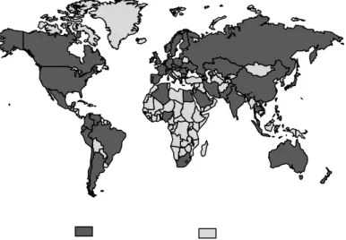
, ) ( ) ( , ) u v w T =

_∑

The FDI data are collected from the Economist Intelligence Unit’s (EIU) Country Data reports, a database that includes 60 regions from 1989 to 2015. The sample regions are depicted in Figure 1 as black. The sample includes 19 Asian, 25 European, three North American, seven South American, four African, and two Oceanian

regions. As can be seen in Figure 1, the sample regions are representative because they include the main global economies, including the US, the European Union, China, Japan, and others. The sample years are from 1989 to 2015, totaling 27 years.

Sample regions Regions not in the sample

Figure 1. Sample Regions

3.2 Network Features

3.2.1 Features of the Global Network

The MSTs of the global financial network are calculated from 1989 to 2015, with the total number of lines for each year shown in Table 1.

Table 1. Total Number of Connected Lines of MSTs

Number 108 108 106 112 116 114 118

Due to space limitations, only the networks of representative years are reported in Figure 2.

1989 1995 2000 2010 2015

Figure 2. Global Financial Network Derived from MST (Representative Years)

According to Table 1 and Figure 2, during the sample period on a global level, the total number of network lines increases slightly from 108 in 1989 to 118 in 1995. The total number of lines is the same after 1995. However, Figure 2 shows that these networks have been developing from having only limited number of large centers to having numerous smaller centers, i.e., revealing a trend toward less concentrated networks. For example, in 1989, there was only one super center in the US with 24 connected lines. For 2015, there were more centers including the Netherlands, France, Japan, Germany, and mainland China. This implies that the United States’ super-center status has weakened over time and that the global financial market has

developed into a multi-centered network. Globally, the total number of network lines has only changed slightly; however, there are increasingly more centers in the world’s interconnected network.

3.2.2 Features of Regions

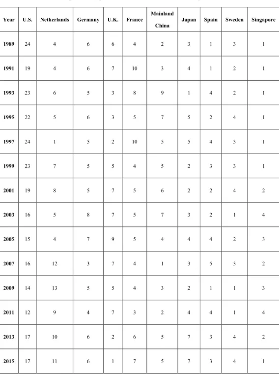
At the regional level, the interconnectedness of each region changes dynamically. Table 2 reports the top-10 regions with the most average connected lines over our sample period.

Table 2. Top-10 Regions with the Most Average Connected Lines

Year U.S. Netherlands Germany U.K. France

Mainland

China Japan Spain Sweden Singapore

1989 24 4 6 6 4 2 3 1 3 1 1991 19 4 6 7 10 3 4 1 2 1 1993 23 6 5 3 8 9 1 4 2 1 1995 22 5 6 3 5 7 5 2 4 1 1997 24 1 5 2 10 5 5 4 3 1 1999 23 7 5 5 4 5 2 3 3 1 2001 19 8 5 7 5 6 2 2 4 2 2003 16 5 8 7 5 7 3 2 1 4 2005 15 4 7 9 5 4 4 4 2 3 2007 16 12 3 7 4 1 3 5 3 2 2009 14 13 5 5 4 3 2 1 1 3 2011 12 9 4 7 3 2 4 4 1 4 2013 17 10 6 2 6 5 7 3 4 2 2015 17 11 6 1 7 5 7 3 4 1

Among these regions, only mainland China is a developing region while all of the others are developed regions. The US is consistently the single super-pivot directly connected to the most regions, although the number of its connecting lines has

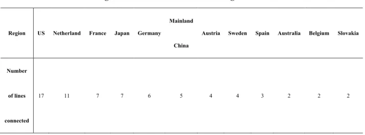
decreased since 2000. On the contrary, the Netherlands shows increasing connections, having reached second place in the rankings since 2007. Germany and France show relatively stable connections while the UK follows a similar path as the US. For the Asia Pacific region, we identify three regions, mainland China, Japan and Singapore, in the top-10 global rankings. Mainland China ranked sixth in 2015, albeit with significant volatility during the sample period. Before 1994, the number of China’s connecting network lines increased rapidly, with a significant drop after 2003, and then China has remained in sixth place globally since 2012. In 2007, the only region directly connected to mainland China was Hong Kong. Recently, the number of network lines that connect to Japan, Spain, and Sweden has significantly increased. Singapore was relatively stable in the 1990s but has experienced volatility since 2000. Table 3 shows all regions with more than one line for 2015. Similarly, except for mainland China, all of the other regions are developed regions. Seventeen regions were directly connected to the US in 2015, implying that it has an irreplaceable status as a pivot. For this period, the regions with which mainland China are mostly

economically connected are Hong Kong, Japan, Korea, Singapore, and Taiwan, thus increasing the likelihood of systemic risk transmitting among them. Table 3 also shows that there are three regions in the Asia Pacific region, specifically mainland

China, Japan and Australia, with their number of connecting lines larger than 1 in 2015.

Table 3. Regions with Number of Lines Larger Than 1 in 2015

Region US Netherland France Japan Germany

Mainland

China

Austria Sweden Spain Australia Belgium Slovakia

Number

of lines

connected

17 11 7 7 6 5 4 4 3 2 2 2

3.2.3 Features of the Greater China Area

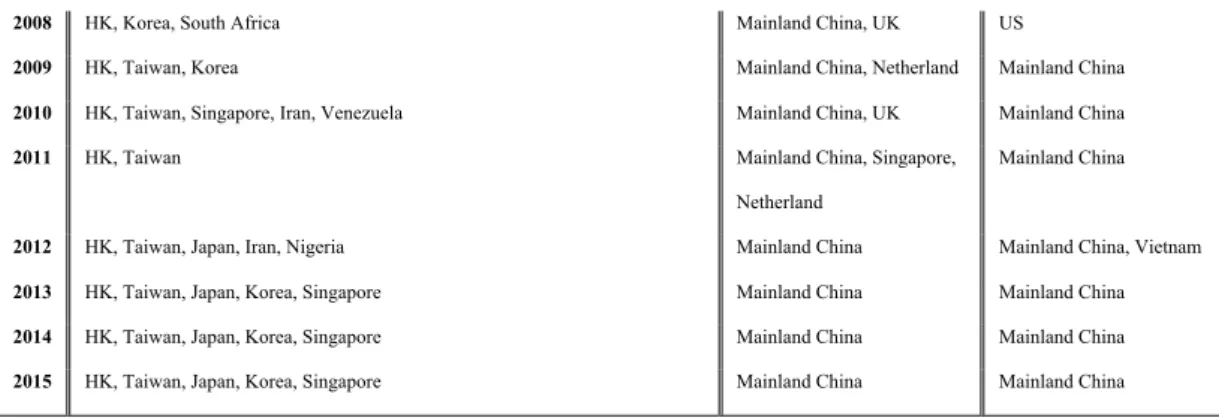
Different regions connect with Greater China each year, mostly within the Pacific Basin area. As Table 4 shows, mainland China, Hong Kong, and Taiwan have a long history of interconnectedness. Hong Kong and mainland China are closely connected and mutually dependent on each other, with implications for the transmission of systemic risk. Before the subprime mortgage crisis in 2008, mainland China had more connections with the Philippines, the US, and Vietnam, but this was not so after the financial crisis. Mainland China has maintained a relatively high degree of

interconnectedness with multiple regions since 1995, especially in the most recent three years.

Correspondingly, Hong Kong connects mainly with mainland China in the sample period. The interconnectedness between Hong Kong and the US was notable only

before and during the financial crisis but diminished after 2008. Mainland China is also the most connected region for Taiwan. Taiwan only connected with the US before 1991, but their direct connection was lost in 1992 when Taiwan began to connect with mainland China. The connection between Taiwan and mainland China was interrupted in 2006 to 2008 but reestablished after 2009.

Therefore, we find significant interconnectedness among mainland China, Hong Kong, and Taiwan. For these three regions, their systemic risk changes

synchronously. Mainland China is the most important region of the Greater China. In most sample years, mainland China is the only connected region for Hong Kong and Taiwan.

Table 4. Regions Connected with Mainland China, Hong Kong and Taiwan Connected with Mainland China Connected with HK Connected with Taiwan 1989 Hong Kong, Japan Mainland China US

1990 HK, Philippines, US Mainland China US

1991 HK, Japan, Philippines Mainland China US

1992 HK, Taiwan, Japan, Korea, Vietnam, Peru Mainland China, Thailand Mainland China

1993 HK, Taiwan, Korea, Philippines, US, Vietnam, KZ, Indonesia, Hungary Mainland China Mainland China

1994 HK, Taiwan, Korea, Philippines, US, Vietnam, KZ, Indonesia, Sri Lanka,

Romania

Mainland China, Thailand Mainland China

1995 HK, Taiwan, Japan, Singapore, Vietnam, Sri Lanka, Ukraine Mainland China Mainland China

1996 HK, Taiwan, Japan, Korea, Singapore Mainland China Mainland China, Vietnam

1997 HK, Taiwan, Japan, Korea, KZ Mainland China Mainland China

1998 HK, Taiwan, Korea, US, Singapore Mainland China Mainland China

1999 HK, Taiwan, Korea, US, Singapore Mainland China Mainland China

2000 HK, Taiwan Mainland China, Singapore Mainland China, Vietnam

2001 HK, Taiwan, Japan, Korea, Philippines, US Mainland China Mainland China, Vietnam

2002 HK, Taiwan, Korea, US Mainland China Mainland China

2003 HK, Taiwan, Japan, Korea, Philippines, Singapore, Iran Mainland China Mainland China

2004 HK, Taiwan, Korea, Philippines Mainland China, US Mainland China

2005 HK, Taiwan, Japan, Korea Mainland China Mainland China

2006 HK, Korea Mainland China, US Netherland

2008 HK, Korea, South Africa Mainland China, UK US

2009 HK, Taiwan, Korea Mainland China, Netherland Mainland China

2010 HK, Taiwan, Singapore, Iran, Venezuela Mainland China, UK Mainland China

2011 HK, Taiwan Mainland China, Singapore, Netherland

Mainland China

2012 HK, Taiwan, Japan, Iran, Nigeria Mainland China Mainland China, Vietnam

2013 HK, Taiwan, Japan, Korea, Singapore Mainland China Mainland China

2014 HK, Taiwan, Japan, Korea, Singapore Mainland China Mainland China

2015 HK, Taiwan, Japan, Korea, Singapore Mainland China Mainland China

3.3 Identification of Systemically Important Regions

According to FIS (2009), interconnectedness is one of the major measures for

systemic importance. It represents the importance of a region in terms of transferring systemic risk. If one region is highly interconnected with others, it is a pivot in the network. To identify SIRs, we define regions with the top 10% most connected lines as systemically important. According to the calculation results of the global networks in each sample year, the top 10% percentile cutoff is four lines. Therefore, in this study SIRs are defined as regions with connected lines equal to or larger than four in each year. Applying this standard, we identify the number of SIRs for each year as shown in Figure 3.

Figure 3. The Number of Systemically Important Regions by Year 5 10 4 5 6 7 8 9 10 1989 1990 1991 1992 1993 1994 1995 1996 1997 1998 1999 2000 2001 2002 2003 2004 2005 2006 2007 2008 2009 2010 2011 2012 2013 2014 2015

Figure 3 shows that the number of SIRs fluctuates over time but increases overall. The increasing magnitude becomes more significant after the subprime mortgage crisis period of 2008. In 2007, there were only five SIRs, including France, the Netherlands, Spain, the UK and the US. The number of SIRs increased rapidly to ten in 2011. The US only showed 16 connected lines in 2007, which is the lowest number in its history. This may be due to other regions’ concerns over a spill-over effect from the United States’ financial crisis; therefore, they might have deliberately reduced their connections with the US. Alternatively, it could be that the American economic situation had actually weakened significantly before the crisis, leading to a contraction of interconnectedness. After the subprime crisis, the number of SIRs at the global level increased significantly, indicating that there were more connected centers in the world. The global economic market seems to be developing into a multi-centered network.

3.4 Concentration of the Global Network

Aside from the number of lines and the number of centers, concentration is another important feature of a network structure and signals the density of the

interconnectedness. We use the Herfindahl-Hirschman Index (HHI)4 of the lines to reflect the degree of concentration, which is defined as follows:

(

)

HHI ASI X RSI

= =

=

_∑

_∑

(1)

4 _{The Herfindahl-Hirschman Index is usually used to measure the degree of concentration in an industry. HHI} equals the sum of the square of market share of each individual financial institution, and can be used to measure the extent of a monopoly. This is similar to our definition of the concentration of networks.

where ASI_itis the number of lines connected in year t for the ith region, which is the extent of Absolute Interconnectedness of the region; X_tis the total number of lines of the network in year t; RSI_it is the proportion of the number of lines of the ith region toX_t, which is defined as the extent of the region’s Relative Interconnectedness. The HHIs of each year are depicted in Figure 4.

Figure 4. HHI of the Global Network

Generally, HHI decreases over time. This indicates that the global network consisted of only a small number of large centers in 1990s and gradually developed into a network with numerous smaller centers in the 2000s, which is consistent with the increase in the number of SIRs over our sample period. In other words, we witness a decrease in the degree of concentration in the global network and an increase in the number of SIRs over the past several decades. Next, we explore the impact of interconnectedness on the transmission of systemic risk.

0.035 0.035 0.040 0.045 0.050 0.055 0.060 0.065 0.070 1989 1990 1991 1992 1993 1994 1995 1996 1997 1998 1999 2000 2001 2002 2003 2004 2005 2006 2007 2008 2009 2010 2011 2012 2013 2014 2015

4. The Impact of Interconnectedness on Systemic Risk

4.1 Measures of Systemic Risk

In this section we study the impact of regional interconnectedness on systemic risk. Most measures of systemic risk focus on financial institutions and their expected shortfalls (Acharya et al., 2017). We argue that the definition of system risk should recognize risk from all sources, including sovereign risk, currency risk, and banking sector risk. Therefore, a more comprehensive variable is needed to measure regions’ systemic risk. We proxy for regions’ systemic risk by using the Country Risk Score of the EIU5, which is denoted as riskit. The riskit is the systemic risk in year t for the ith

region. According to the EIU, the Country Risk Score comprehensively reflects sovereign risk, currency risk, and banking sector risk. The higher the riskit, the higher

the systemic risk. The descriptive statistics of riskit are presented in Table 5. As the

Country Risk Score only starts from 1997, and as there are some missing values, we finally obtain a total of 1,075 observations.

Table 5. Descriptive Statistics of Country Risk Scores

Regions Sample years

Number of

Observations Mean

Std.

Dev. Min Median Max Skewness Kurtosis

60 19 1075 37.88 14.97 9 38 74 0.19 2.12

5 _{The EIU-designed EIU Risk Model produces the systemic risk rate for all regions. This is the most authoritative ratio for measuring the}

4.2 Impact of Concentration on Systemic Risk at the Global Level

We first apply orthogonal pulse analyses to test Hypothesis 1, investigating the impact of network concentration on systemic risk at the global level. The orthogonal pulse function is widely used to study the effect of one variable on others (Berument & Froyen, 2009; Pradhan 2015). This function not only shows the direction of the effect, but also shows its time lag and significance level in each year. This implies that when all of the other variables and residuals remain the same, the effect of a one unit increase in the residual of the jth variable in time t (𝜀_"#) on the value of the ith variable at time t+s (𝑦_',#)*), i.e. the orthogonal pulse function, is a function of the time lag s: ∂𝑦_',#)*/ ∂ε_"#.

We first study the impact of network concentration on systemic risk at the global level. The response variable riskit is the systemic risk of region i in year t. Here,

shocks come from changes in the concentration of the global network, i.e. HHIt. The

results of the orthogonal pulse are depicted in Figure 5. The horizontal axis represents the time lag after the shock, while the vertical axis represents the number of crises in the sample regions for that year. The two thin black lines are the upper and lower bound of the 95% confidence interval and the bold black line represents the average.

Figure 5. Dynamic Impact of HHI of Lines on Global Systemic Risk

In Figure 5, the HHI of lines initially produces a significantly positive effect on global systemic risk, and then the HHI diminishes to insignificance after five years.

Therefore, we find strong evidence supporting Hypothesis 1, which proposed that that the more concentrated the network, the higher the global systemic risk. Our empirical results suggest that a multi-centered global economic network, rather than a single pivotal center, can reduce systemic risk at the global level.

4.3 Interconnectedness of Systemic Risk at the Regional Level

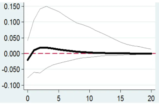
In this section we test Hypothesis 2, again using orthogonal pulse analyses. More specifically, we explore whether and how the number of connected lines, i.e., interconnectedness, influences the systemic risk of regions. As SIRs and NSIRs are expected to show different characteristics and performances, we split the whole sample into two groups: SIRs and NSIRs. We use the orthogonal pulse function to obtain the impact of regions on systemic risk from the number of connected lines. In Figure 6, the horizontal axis represents the time lag after the shock, while the vertical axis represents the systemic risk for the same group of regions for that year. The two thin black lines are the upper and lower bound of the 95% confidence interval and the bold black line represents the average. There are three graphs for Figure 6. Figure 6a shows the results for the whole sample, while Figure 6b and 6c are for NSIRs and SIRs, respectively.

(a) Whole Sample

(b) NSIR (c) SIR

Figure 6. Dynamic Impact of Interconnectedness on NSIRs’ Systemic Risk

Figure 6 shows that interconnectedness significantly increases systemic risk only for NSIRs because the lower bound of the confidence interval is significantly larger than 0 at the 5% level. However, it is not significant for SIRs and the whole sample.6 More specifically, our results indicate that for NSIRs an increase in the number of connected lines increases the possibility of systemic risk in the long run. Therefore, an increase in interconnectedness leads to higher systemic risk for NSIRs, i.e. the

negative effect of the greater possibility of being contaminated by other regions

6 _{The results of ASI and RSI are similar, so we only report those of ASI. The results of RSI are available upon} request from the authors.

dominates the positive effect of the potential transfer of risk to other regions. When there is an additional region directly connected to a certain NSIR, systemic risk decreases slightly in the short run. However, after one year, systemic risk increases rapidly and remains significantly positive at the confidence level of 95%, peaking at 0.04 after two years. In other words, the average Country Risk Score increases by 0.04 in the second year after the shock. After that, the effect of the positive shock declines and then converges to 0 after 10 years.

The underlying reason for the difference in significance between SIRs and NSIRs is perhaps that NSIRs have a limited number of connected lines. This implies a limited number of available channels for NSIRs to diversify and transfer risk out of their region. Once NSIRs become more interconnected, the negative effect of

contamination of systemic risk from other regions dominates the positive effect of transferring systemic risk. In contrast, SIRs have more channels for transferring risk. This suggests that the positive effect of connectedness is stronger for SIRs than for NSIRs, and the positive effect cancels out the negative effect of contamination possibility for SIRs. Therefore, Hypothesis 2 is only partially supported. At the

regional level, the interconnectedness of NSIRs aggravates the impact of systemic risk on a specific region. We do not find a significant relationship between

interconnectedness and systemic risk for SIRs. Our results suggest that with regard to systemic risk management, interconnectedness or openness is not always beneficial for NSIRs. Different regions should choose appropriate strategies for managing

systemic risk according to their own characteristics. Overall, our results suggest that an increase of systemic risk for a few regions might potentially reduce aggregate systemic risk at the global level. Measuring systemic risk at the level of individual institutional firms could be misleading because it comes at the cost of increasing systemic risk for the entire system. These findings have not been discussed in the literature and should be of interest to policymakers and regulators.

5. The Main Causes of the Difference in Interconnectedness between SIRs and NSIRS

Previous analysis shows that when NSIRs’ interconnectedness increases, their

systemic risk also increases. However, we do not find similar evidence for SIRs. One potential reason is that SIRs have stronger connections that can spread risk and provide protection from that risk. However, there is a cost to decreasing systemic risk by simply reducing NSIRs’ interconnectedness. This cost results from going against the direction of globalization and produces numerous side effects, such as a decrease in social welfare (Ahmadi, 2003) and the stimulation of competition,

entrepreneurship, and economic growth (Ching et al., 2011). One potential solution for NSIRs, so that they can increase their interconnectedness while not simultaneously increasing their systemic risk, is to develop themselves into SIRs. Our results suggest that SIRs are in a better position to isolate themselves from systemic risk. We thus attempt to identify some key factors that affect interconnectedness, so that it becomes possible for NSIRs to increase their interconnectedness through these channels. The literature suggests that the global importance of a region, in terms of the systemic risk

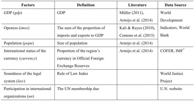
of contagion, depends on various factors including the size of the economy, trading, industrial structure, currency, and the legal system, among other factors. We consider eight factors as listed in Table 6. After removing their missing values, we obtain 858 observations for 51 regions from 1995 to 2015.

Table 6. Factors Affecting Interconnectedness

Factors Definition Literature Data Source

GDP (gdp) GDP Müller (2011), Armijo et al. (2014) World Development Indicators, World Bank

Openess (imex) The sum of the proportion of imports and exports to GDP

Kali & Reyes (2010), Centeno et al. (2015) Population (popu) Size of population Armijo et al. (2014) International status of the

currency (currency)

Proportion of the region’s currency in Official Foreign Exchange Reserves

Armijo et al. (2014) COFER, IMF7

Soundness of the legal system (law)

Rule of Law Index World Justice Project Participation in international

organizations (un)

The UN membership due U.N. website

The Oaxaca-Blinder decomposition is used here to calculate each factor’s proportion of contribution to the difference between SIRs and NSIRs (Oaxaca & Ransom, 1994; González Álvarez & Barranquero, 2009). We use the two-fold method (Jann, 2008) to decompose the difference in interconnectedness between SIRs and NSIRs:

𝐷𝑖𝑓𝑓𝑒𝑟𝑒𝑛𝑐𝑒 = [𝐸 𝐹_9: − 𝐸 𝐹_<9: ]′𝛽∗_{+ [𝐸 𝐹}

9: ′ 𝛽9: − 𝛽∗ + 𝐸 𝐹<9: ′ 𝛽∗− 𝛽<9: ] (2) The first part on the right hand side comprises the explanatory variables listed in Table 6, while the second part comprises all of the other factors that are difficult to

measure or that involve unavailable data, such as political, social, cultural, and

religious factors. We mainly consider the factors that are measurable in Table 6 based on the literature. The results from the Oaxaca-Blinder Decomposition are presented in Table 7.

Table 7 suggests that there are significant differences in SIRs and NSIRs in many aspects. Overall, the factors considered in our model contribute 42.01% to the total difference in interconnectedness, significant at the 1% level. Thus our model has satisfactory explanatory power for the difference in interconnectedness between SIRs and NSIRs. GDP contributes 38.34% to the total difference and is significant at the 1% level. We find that a high GDP is the main cause of SIRs being more connected than NSIRs. The second factor is status of currency, contributing 12.77%, which is also significant at the 1% level. This indicates that the currencies of SIRs usually have higher international status, making SIRs more connected. However, the contribution of population is negative, -2.32%, and significant at the 1% level. This indicates that NSIRs, which are less connected, perform better with large populations, increasing NSIRs’ interconnectedness.8 NSIRs are usually developing regions with relatively large populations. Thus, we find some empirical evidence suggesting that a large population is positively related to interconnectedness. Other factors are not significant in explaining the difference in interconnectedness between SIRs and NSIRs in our model. Our results suggest that it is beneficial for NSIRs to increase their

8 _{Oaxaca & Ransom (1994) suggest that a negative sign indicates that the inferior group (NSIRs) outperforms the} superior group (SIRs), and this factor narrows the gap between these two groups (Alvarez & Barranquero, 2009).

interconnectedness through three main channels: developing their economy

(increasing GDP), improving their currency’s international status; and increasing the size of their population. When NSIRs can evolve into SIRs, they become financially stronger and more connected to global network channels, thereby reducing their vulnerability to systemic risk.

Table 7. Results of the Oaxaca-Blinder Decomposition

Coefficient t- value Percentage

Systemically Important Regions 7.4127*** 17.88 Non-Systemically Important Regions 1.2787*** 62.62

Total Difference 6.1340*** 14.78 100.00% gdp 2.3518*** _{5.41 38.34%} imex -0.0140 -0.77 -0.23% popu -0.1423*** _{-2.94 -2.32%} currency 0.7833*** _{4.25 12.77%} law -0.0487 -1.08 -0.79% un -0.3530 -1.00 -5.75% Explainable Part 2.5771*** _{6.73 42.01%} Other Part 3.5569*** _{12.12 57.99%} Con. -8.4607** -2.22 N 858

6. Conclusion and Recommendations

This study applies a minimum spanning tree (MST) technique to develop an annual network structure of countries and regions and to identify systemically important regions (SIRs). The number of lines connected to each region and the HHI index were used to measure network interconnectedness and concentration. The SIRs and NSIRs are identified according to the interconnectedness of different regions. At the global level, we analyze the effect of network concentration on systemic risk. At the regional level, we proceed to study the effect of the number of connected lines on regional systemic risk. Finally, the main causes of the difference in interconnectedness between SIRs and NSIRs are identified using the Oaxaca-Blinder decomposition technique.

In this study, we report the following three findings. First, there is a global network that connects all of the world’s regions, with pertinent data available on an annual basis. Systemic risk is transferred through the MST network. In the global network, the total number of lines does not change significantly in our sample years. However, this global network has become less concentrated. Its single pivotal center has given way to a multi-centered structure, and a similar transition is visible for the US in an earlier period. Second, the structure of the global network significantly affects

systemic risk: the more concentrated the network, the higher the systemic risk. At the regional level, the more connected the NSIRs, the higher the systemic risk. However, for SIRs we do not find evidence showing that interconnectedness significantly

affects systemic risk. Therefore, the best approach for NSIRs to potentially increase their interconnectedness while protecting themselves from systemic risk is to

transform themselves into SIRs. Third, by developing the economy through channels such as increasing GDP and strengthening the international status of their currencies, NSIRs can eventually evolve into SIRs. Also, a high population density benefits NSIRs by increasing their interconnectedness and making them less vulnerable to systemic risk.

This is the first study to introduce the idea that systemic risk should be primarily measured at the global level instead of at the level of individual financial institutions. Our empirical results suggest that it is potentially beneficial, for global systemic risk management, to construct a less concentrated network with multiple centers, thus moderating the super pivotal status of the US. This lessening of network

concentration can potentially mitigate global systemic risk by having the whole network more easily absorb risk through an increased number of SIRs. An increase of systemic risk for a few regions at the regional level can actually reduce aggregate systemic risk at the global level. Therefore, measuring systemic risk at the level of financial institutions could be problematic because it comes at the cost of increasing systemic risk for the entire system. These findings have important policy implications in the current era of globalization.

We also pay specific attention to the Asia Pacific region, especially the Greater China area because it is now the second largest economic body in the world and the largest

emerging market. Mainland China is still struggling to become an SIR. During this study’s sample period, mainland China represents an SIR in 1992-1999, 2001-2005, 2010, and 2012-2015, and an NSIR in 2000, 2006-2009, and 2011, suggesting that its SIR status is unstable over time. Mainland China should monitor the changes in its connections with other regions, track its status in the global network, guard against potentially negative effects, and aim to become a stable SIR. Our empirical evidence suggests that negative influence can be avoided or mitigated if a region becomes stronger and attains a higher global status. Hong Kong and Taiwan are both NSIRs and are generally only connect with mainland China. Thus, Hong Kong and Taiwan should closely monitor their connections with mainland China. All three regions are interconnected as a whole sub-system, and systemic risk from any one of them can spread to the others directly or indirectly. Meanwhile, Hong Kong and Taiwan might be exposed to systemic risk if they adopt an open policy without appropriate

procedures. Our results suggest that NSIRs should establish mechanisms to defend against risk and maintain a reasonable level of interconnectedness with other regions.

References:

1. Acemoglu D, Carvalho VM, Ozdaglar A, Tahbaz-Salehi A., 2012. The network origins of aggregate fluctuations. Econometrica 80, 1977-2016.

2. Acemoglu, D., Ozdaglar, A., Tahbaz-Salehi, A, 2017. Microeconomic origins of macroeconomic tail risks. Am. Econ. Rev. 107, 54-108.

3. Acemoglu, D., Ozdaglar, A., Tahbaz-Salehi, A, 2015. Systemic risk and stability in financial networks. Am. Econ. Rev. 105, 564-608.

4. Acharya, V., Pedersen, L. H., Philippon, T., Richardson, M., 2017. Measuring systemic risk. Rev. Financ. Stud. 30, 2-47.

5. Ahmadi, N. 2003. Globalisation of consciousness and new challenges for international social work. Int. J. Soc. Welf. 12, 14-23.

6. Allen, F., Gale, D., 2000. Financial contagion. J. Polit. Econ. 108, 1-33.

7. Armijo, L. E., Mühlich, L., Tirone, D. C., 2014. The systemic financial importance of emerging powers. J. Policy Model. 36, S67-S88.

8. Barrell, R., Pain, N., 1997. Foreign direct investment, technological change, and economic growth within Europe. Eco. J. 107, 1770-1786.

9. Bathelt, H., Li, P. F., 2013. Global cluster networks—foreign direct investment flows from Canada to China. J. Econ. Geogr. 14, 45-71.

10. Belloumi, M., 2014. The relationship between trade, FDI and economic growth in Tunisia: An application of the autoregressive distributed lag model. Economic Systems 38, 269-287.

11. Berument, H., Froyen, R., Monetary policy and U.S. long-term interest rates: How close are the linkages? Journal of Economics and Business 61, 34-50.

12. Billio, M., Getmansky, M., Lo, A. W., Pelizzon, L., 2012. Econometric measures of connectedness and systemic risk in the finance and insurance sectors. J. Financ. Econ. 104, 535-559.

13. Bisias, D., Flood, M.D., Lo, A.W., Valavanis, S., 2012. A survey of systemic risk analytics. Annu. Rev. Financ. Econ. 41, 255–296

14. Blume, L., Easley, D., Kleinberg, J., Tardos, É., 2013. Network formation in the presence of contagious risk. ACM Transactions on Economics and Computation 1, 6.

15. Blume, L., Easley, D., Kleinberg, J., Tardos, É., 2011. Which networks are least susceptible to cascading failures? Foundations of Computer Science (FOCS), 2011 IEEE 52nd Annual Symposium on. IEEE, 2011: 393-402.

16. Bottazzi, G., De Sanctis, A., Vanni, F., 2016. Non-performing loans, systemic risk and resilience in financial networks. Laboratory of Economics and Management (LEM), Sant’ Anna School of Advanced Studies, Pisa, Italy.

17. Cabrales, A., Gottardi, P., Vega-Redondo, F., 2017. Risk sharing and contagion in networks. Rev. Financ. Stud. 30, 1-71.

18. Cai, J., Eidam, F., Saunders, A., Steffen, S., 2018. Syndication, interconnectedness, and systemic risk. J. Financ. Stabil. 34, 105-120.

19. Castiglionesi, F., Eboli, M., 2015 Liquidity flows in interbank networks. International IFABS Conference, Lisbon, Portugal.

20. Centeno, M. A., Nag, M., Patterson, T. S., Shaver, A., Windawi, A.J., 2015. The emergence of global systemic risk. Annu. Rev. Sociol. 41, 65-85.

21. Ching, H.S., Hsiao, C., Wan, S.K., Wang, T. 2011. Economic benefits of globalization: the impact of entry to the WTO on china's growth. Pac. Econ. Rev. 16, 285-301.

22. Eboli, M., 2013. A flow network analysis of direct balance-sheet contagion in financial networks. Working Paper No. 1862, Kiel Institute for the World Economy. 23. Elliott, M., Golub, B., Jackson, M. O., 2014. Financial networks and contagion.

Am. Econ. Rev. 104, 3115-3153.

24. Fouque, J., Langsam, J.A., 2013. Handbook on Systemic Risk. Cambridge University Press, Cambridge.

25. Freixas, X., Parigi, B. M., Rochet J. C., 2000. Systemic risk, interbank relations, and liquidity provision by the central bank. J. Money Credit Bank 32, 611-638. 26. FSB, IMF and BIS, 2009. Guidance to Assess the Systemic Importance of

Financial Institutions, Markets and Instruments: Initial Considerations. Federal Reserve Bank Background Paper.

27. Gai, P., Andrew, H., Sujit, K., 2011 Complexity, concentration and contagion. J. Monetary Econ. 58, 453–70.

28. Garratt, R., Mahadeva, L., Svirydzenka, K., 2011. Mapping systemic risk in the international banking network. Bank of England, 2011.

29. Giglio, S., Kelly, B., Pruitt, S., 2016. Systemic risk and the macroeconomy: An empirical evaluation. J. Financ. Econ. 119, 457-471.

30. Glasserman, P., Young, H. P., 2015. How likely is contagion in financial networks? J. Bank Financ. 50, 383-399.

31. González Álvarez, M., Barranquero, A.C., 2009. Inequalities in health care utilization in Spain due to double insurance coverage: An Oaxaca-Ransom decomposition. Soc. Sci. Med. 69, 793-801.

32. Haldane, A. G., 2009. Rethinking the financial network. Bank of England, Speech delivered at the Financial Student Association, Amsterdam. Available in http://www.bankofengland.co.uk/publications/calendar/2009/april.htm (accessed 2011).

33. Holland, D., Pain N., 1998. The diffusion of innovations in Central and Eastern Europe: A study of the determinants and impact of foreign direct investment. London: National Institute of Economic and Social Research.

34. Jann, B, 2008. The Blinder-Oaxaca decomposition for linear regression models. The Stata Journal 8, 453-479.

35. Kali, R., Reyes, J., 2010. Financial contagion on the international trade network. Econ. Inq. 48, 1072-1101.

36. Liu, H., Modarres, R., 2017. Modeling a minimal spanning tree. Commun. Stat.-Simul. Comput. 46, 5246-5256.

37. Markose, S, Giansante, S., Shaghaghi, A. R., 2012. ‘Too interconnected to fail’ financial network of U.S. CDS market: Topological fragility and systemic risk. J. Econ. Behav. Organ. 83, 627-646.

38. Müller, M., 2011. Approaches in dealing with systemically important financial institution. Working Paper.

39. Nier, E., Yang, J., Yorulmazer, T. Alentorn, A., 2007. Network models and financial stability. J. Econ. Dyn. Control 31, 2033-2060.

40. Oaxaca, R. L., Ransom, M. R., 1994. On discrimination and the decomposition of wage differentials. J. Econom. 61, 5-21.

41. Ouyang, H., Liu, X., 2014. Study on systemic importance of financial institutions based on network analysis. Management World 8, 171-172.

42. Pain, N., Wakelin, K., 1998. Export performance and the role of foreign direct investment. The Manchester School 66 (S), 62-88.

43. Plosser, C. I., 2009. Restoring financial stability: How to repair a failed system. Speech at the New York University Conference.

44. Pradhan, K. P., 2015 Orthogonal pulse based wideband communication for high speed data transfer in sensor applications. The University of Alabama at Birmingham.

45. Schweitzer, F., Fagiolo, G., Sornette, D., Vega-Redondo, F., Vespignani, A., White, D.R., 2009. Economic networks: The new challenges. Science 325, 422-425. 46. Vivier-Lirimont, S., 2006. Contagion in interbank debt networks. Working Paper. 47. Xu, Q., Chen, L., Jiang, C., Yuan, J., 2018. Measuring systemic risk of the banking

industry in China: A DCC-MIDAS-t approach. Pac-Basin Financ. J. 51, 13-31. 48. Yellen, J., 2013. Interconnectedness and systemic risk: Lessons from the financial

crisis and policy implications. A speech at the American Economic Association/American Finance Association Joint Luncheon, San Diego, California, Board of Governors of the Federal Reserve System (US).

49. Yun, J., Moon, H., 2014. Measuring systemic risk in the Korean banking sector via dynamic conditional correlation models. Pac-Basin Financ. J. 27, 94-114.